Biogeography Meets Niche Modeling: Inferring the Role of Deep Time Climate Change When Data Is Limited

Culshaw, Victoria; Mairal, Mario; Sanmartín, Isabel

doi:10.3389/fevo.2021.662092

ORIGINAL RESEARCH article

Front. Ecol. Evol., 21 September 2021

Sec. Biogeography and Macroecology

Volume 9 - 2021 | https://doi.org/10.3389/fevo.2021.662092

Biogeography Meets Niche Modeling: Inferring the Role of Deep Time Climate Change When Data Is Limited

$\r\nVictoria Culshaw,*$ Victoria Culshaw^1,2*

Mario Mairal³

Isabel Sanmartín^1*

¹Real Jardín Botánico (RJB), CSIC, Madrid, Spain
²Department of Ecology and Ecosystem Management, Technische Universität München (TUM), Munich, Germany
³Departamento de Biodiversidad, Ecología y Evolución, Facultad de Biología, Universidad Complutense de Madrid, Madrid, Spain

Geographic range shifts are one major organism response to climate change, especially if the rate of climate change is higher than that of species adaptation. Ecological niche models (ENM) and biogeographic inferences are often used in estimating the effects of climatic oscillations on species range dynamics. ENMs can be used to track climatic suitable areas over time, but have often been limited to shallow timescales; biogeographic inference can reach greater evolutionary depth, but often lacks spatial resolution. Here, we present a simple approach that treats them as independent and complementary sources of evidence, which, when used in partnership, can be employed to reconstruct geographic range shifts over deep evolutionary timescales. For testing this, we chose two extreme African disjunctions: Camptoloma (Scrophulariaceae) and Canarina (Campanulaceae), each comprising of three species disjunctly distributed in Macaronesia and eastern/southern Africa. Using inferred ancestral ranges in tandem with preindustrial and paleoclimate ENM hindcastings, we show that the disjunct pattern was the result of fragmentation and extinction events linked to Neogene aridification cycles. Our results highlight the importance of considering temporal resolution when building ENMs for rare endemics with small population sizes and restricted climatic tolerances such as Camptoloma, for which models built on averaged monthly variables were more informative than those based on annual bioclimatic variables. Additionally, we show that biogeographic information can be used as truncation threshold criteria for building ENMs in the distant past. Our approach is suitable when there is sparse sampling on species occurrences and associated patterns of genetic variation, such as in the case of ancient endemics with widely disjunct distributions as a result of climate change.

Introduction

The current concern on anthropogenic-induced climate change and its impact on biodiversity levels has increased the interest in reconstructing organisms’ responses to past climatic events. Geographic range shifts, where species track their climatic niche under events of rapid climate change, are expected if the rate of environmental change is greater than that of species’ ability to adapt to the new conditions (Martínez-Meyer and Peterson, 2006; Thuiller et al., 2006; Waldron, 2010). These shifts can result in smaller population sizes, reduced genetic diversity, and a higher extinction risk (Waldron, 2010; Mairal et al., 2018). Furthermore, limited gene flow increases inter-population genetic differences and may eventually drive speciation (Dorn et al., 2014).

Studies on climate change and its effects on species range dynamics have typically focused on recent geological timescales, such as the glacial and interglacial stages of the Pleistocene, the last 2.6 million years (Hewitt, 2004), or the last 120,000 years of the Late Pleistocene-Holocene (Martínez-Meyer et al., 2004; Martínez-Meyer and Peterson, 2006; Espíndola et al., 2012; Mairal et al., 2018). However, these shallow timescales are often insufficient to discern how much evolutionary history loss is anthropogenic-induced or a result of the natural cycling of diversification rates in long-term species dynamics (Moen and Morlon, 2014; Huang et al., 2015). In contrast, evolutionary data that spans deeper timescales, e.g., tens of millions of years, is expected to provide a more accurate understanding of organisms’ persistence and adaptational responses, which are built over generations of genetic changes (Willis and MacDonald, 2011; Svenning et al., 2015; Meseguer et al., 2018; Burke et al., 2018), and hence, a more accurate prediction on the impact of ongoing and future climate change on a species geographic range (Martínez-Meyer et al., 2004; Diniz-Filho and Bini, 2008; Romdal et al., 2013; Meseguer et al., 2015; Burke et al., 2018). One climate change event of major scientific and societal concern is the current aridification trend that affects areas such as the African continent, the Mediterranean Basin and Arabia-Western Asia (Berdugo et al., 2020). Causes are both historical and contemporary: geotectonic changes starting in the Late Neogene, the last 25 million years, introduced a drier climate in the southwest Palearctic, with increasing annual temperatures and decreasing precipitation levels, which led some lineages to extinction (Trauth et al., 2008; Pokorny et al., 2015) also human-induced greenhouse emissions and deforestation also contributed to this trend by dramatically reducing species ranges (Mairal et al., 2018; Berdugo et al., 2020).

Two approaches are often used to reconstruct the evolutionary signature of climate change on species range dynamics. Biogeographic inferences, based on a time-calibrated phylogeny and associated taxa distributions, can be used to infer ancestral geographic ranges and the sequence of geographic range shifts that led to the current distributions (Ree and Smith, 2008; Ronquist and Sanmartín, 2011). Ecological niche models (ENM), based on occurrence data, can be used to estimate the environmental preferences (climatic envelope) of species, allowing for spatial exploration of similar climate conditions in the past, present, and future (Araújo and New, 2007; Meseguer et al., 2015; Mairal et al., 2017; Carboni et al., 2018; Hæuser et al., 2018). The two approaches have their advantages and shortcomings. Biogeographic inference typically employs pre-defined discrete areas that are represented by abstract units (e.g., A, B, and AB) instead of bounded by geographical coordinates (Ree and Sanmartín, 2009; but see Quintero et al., 2015). ENMs implicitly assume that an organism’s climatic niche is conserved over evolutionary time, which might be unrealistic under repeated cycles of ciimate change and over long timescales (Peterson, 2006). The use of ENMs to hindcast across time is also limited by the availability of paleoclimatic data, and most ENMs have been projected onto the recent geological past (Pleistocene, Martínez-Meyer et al., 2004; Mairal et al., 2018; but see Meseguer et al., 2015 and Mairal et al., 2017).

Biogeographic inference and ENMs are not mutually exclusive; there have been attempts to integrate them, even at deep timescales. For example, some authors used ENMs to inform biogeographic analyses and include climatically suitable areas outside the species current range, i.e., due to extinction or incomplete sampling (Yesson and Culham, 2006; Smith and Donoghue, 2010); in other studies, hindcasted ENMs were used to discover transient climatic corridors that facilitated species geographic movement by connecting patches of suitable habitat (Metcalf et al., 2014; Meseguer et al., 2015). These approaches are well suited for medium to large-sized phylogenies (>20 taxa) and groups that are well represented in georeferenced datasets (Smith and Donoghue, 2010; Meseguer et al., 2015). However, in cases where the phylogeny is small (<10 taxa), these methods can be more difficult to implement because of the uncertainty in the inferred ancestral ranges (Sanmartín and Meseguer, 2016). Building ENMs on taxa with sparse and or biased georeferenced occurrence data, such as rare endemics (Rabinowitz, 1981), is also problematic because of the treatment of pseudoabsences, i.e., creation of pseudoabsences to combat the lack of valid (confirmed) absence data (Engler et al., 2004). As well as a quantity problem (i.e., number of records), there is a quality problem (i.e., location accuracy; Engler et al., 2004) because rare endemics are often represented in herbaria collections by voucher specimens with imprecise geographic information. If the rarity of species is associated with ancient origins and long phylogenetic internodes, as in the case of historically high extinction rates, uncertainty in biogeographic inference becomes even larger (Sanmartín and Meseguer, 2016).

Here, we present an approach that, unlike previous approaches does not rely on integrating ENMs into biogeographic analysis (Smith and Donoghue, 2010; Meseguer et al., 2015), but treats them instead as independent and complementary sources of evidence, which, when used in tandem, can fill their respective information gaps. Our approach is most useful in cases when there is high uncertainty in biogeographic analysis associated to a small-sized phylogeny with deep temporal divergences, and when sparse and/or biased georeferenced records make the treatment of pseudoabsences in presence/absence ENM methods difficult (Allouche et al., 2006; Diniz-Filho et al., 2010). We also introduce a new approach in the selection of truncation threshold values for generating binary ENM models in the distant past, which is based on the use of biogeographic inference information.

To test our approach, we used two species-poor angiosperm genera that exhibit a pattern of continent-wide geographic disjunctions attributed to historical climate change. The Rand Flora (Figure 1) describes a floristic pattern in which sister-species, or clades of closely related species, are distributed on opposite sides of the African continent (northwest, eastern, and southern Africa) and adjacent archipelagos, Macaronesia and Socotra (Sanmartín et al., 2010). Recent studies based on phylogenetic and biogeographic data explained this pattern as a result of ecological vicariance and climate-driven extinction linked to an aridification trend that started in the Neogene and continues today (Mairal et al., 2015, 2017; Pokorny et al., 2015; Culshaw et al., 2021; Rincón-Barrado et al., 2021). Genus Camptoloma (Scrophulariaceae) comprises three species: the southwestern African endemic C. rotundifolium, which is sister to a clade formed by Gran Canarian C. canariense and C. lyperiiflorum, endemic to the Horn of Africa, southern Arabia and Socotra Island (Figure 1A; Culshaw et al., 2021). Canarina (Campanulaceae) comprises also three species: the locally widespread Canarian endemic C. canariensis, which is sister to a clade formed by two Eastern African montane species: C. eminii and C. abyssinica (Figure 1B; Mairal et al., 2015, 2018). In addition to their widely disjunct distribution separated by thousands of kilometers across northern and central Africa, Camptoloma and Canarina exhibit deep-temporal divergences, dating back to the Miocene and Pliocene, among the three disjunct species as well as with their recent common ancestors (Mairal et al., 2015; Culshaw et al., 2021). The African species of these two genera are also characterized by small and geographically restricted populations, which in the case of Canarina species are locally threatened by human action (Mairal et al., 2018). Fieldwork and specimen collection in these species is problematic due to political conflict (e.g., Somalia and Yemen) or difficult geographic access (Socotra, Namibian Brandberg Mountains), which likely explain their poor representation in worldwide herbaria and global geographic databases such as GBIF¹. Thus, Canarina and Camptoloma fulfill the three criteria defined above to test our in-tandem biogeographic/ENM approach: a small-sized phylogeny (three species) with long internodal branches (ancient divergence times), and a sparse biased geographic sampling, spanning a broad and continent-wide disjunct distribution.

FIGURE 1

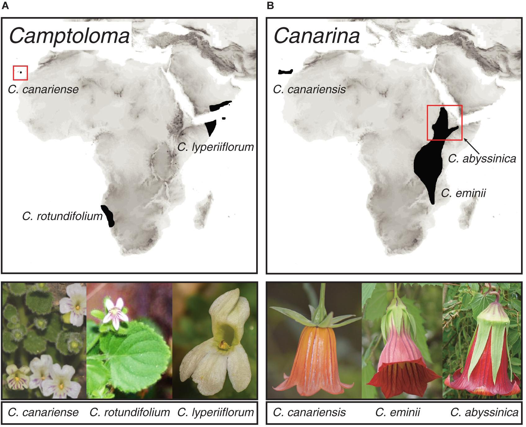
Figure 1. Geographic distribution of species within genera (A) Camptoloma and (B) Canarina, depicting the Rand Flora disjunct distribution across Africa. Photographs: Camptoloma rotundifolium: Martin Weigand; Camptoloma lyperiiflorum: Morten Ross; Canarina canariensis: Mario Mairal; Canarina eminii and Canarina abyssinica: Juan Jose Aldasoro.

The aims of our study were: (i) to build ENM models for genera Canarina and Camptoloma using all available georeferenced occurrence data, present-day and paleoclimatic data, and biogeographic information (i.e., ancestral ranges); the latter were used to select the truncation threshold value needed for converting ENM continuous habitat suitability predictions into binary presence/absence maps that are more readily interpretable. (ii) To reconstruct the sequence of range shifts that led to the current distributions using the ancestral ranges inferred through biogeographic analysis, in tandem with preindustrial and paleoclimate ENM hindcasted projections; specifically, ENM paleoclimate projections were used to reduce uncertainty in the biogeographic analysis by providing information on climatically suitable areas at different time points along the long internodal branches that lead to species divergences. (iii) Finally, the two selected Rand Flora genera offer us an opportunity to explore the effects of ancient climate change on species range dynamics.

Materials and Methods

Biogeographic Inference

We retrieved biogeographic information, i.e., the geographic range of ancestral species and the potential sequence of biogeographic events that led to the current distribution in Camptoloma and Canarina, from our own published studies: Culshaw et al. (2021) and Mairal et al. (2015), respectively. These studies used molecular phylogenies based on several plastid markers and multi-copy nuclear ITS to reconstruct phylogenetic relationships among the disjunct species and their closely related outgroups. Lineage divergence times were inferred using Bayesian relaxed molecular clocks. Biogeographic inference was performed using two parametric approaches that are based on continuous-time Markov-chain (CTMC) models of range evolution with states representing user-defined, discrete areas of distribution (Sanmartín, 2020). Mairal et al. (2015) employed the Bayesian Island Biogeography (BIB) model (Sanmartín et al., 2008), which assumes single-area ancestors and focuses on the sequence of migration events between areas. Culshaw et al. (2021) used the Dispersal Extinction Cladogenesis (DEC) model (Ree and Smith, 2008), which permits widespread ancestors and focuses on scenarios of range division at nodes. CTMC models were implemented in a Bayesian framework using software BEAST (Lemey et al., 2009; Mairal et al., 2015) and RevBayes (Landis et al., 2018; Culshaw et al., 2021), allowing inference of marginal posterior probabilities (mean and 95% high-posterior credibility intervals) for the CTMC parameters and ancestral ranges. In both Camptoloma and Canarina, the geographic range of the stem ancestor, i.e., the divergence between each genus and its sister-group, was inferred with high uncertainty. This is linked to long internodal branches subtending the stem- and crown-nodes in the two genera (Mairal et al., 2015; Culshaw et al., 2021). More details on these analyses can be found in the original studies.

Ecological Niche Models

ENMs for genera Camptoloma and Canarina were generated de novo for this study by following the below steps:

Georeferenced Occurrence Data

Species location data associated with geographical coordinates were obtained individually for Camptoloma and Canarina using: (i) herbarium sample vouchers from the collections of Real Jardín Botánico (MA), Royal Botanical Garden of Edinburgh (E), Uppsala Museum of Evolution Herbarium (U), and Pretoria National Herbarium (PRE); (ii) samples collected during our fieldwork campaigns between 2013 and 2019, mostly in the Canary Islands (details in Mairal et al., 2015 and Culshaw et al., 2021); and (iii) online georeferenced databases, including GBIF (downloaded for Camptoloma from https://doi.org/10.15468/dl.abs9dk; and for Canarina from https://doi.org/10.15468/dl.9fcg75), the ‘‘Flora de Gran Canaria’’², and ‘‘Anthos’’³. Sampling was uneven across species within genera: for Camptoloma, the denser sampling corresponded to Gran Canarian C. canariense, and the least representative to the two African species, especially in regards to georeferenced online records in northern Namibia and Horn of Africa. In Canarina, C. abyssinica was the least represented species in the occurrence dataset. Nevertheless, we emphasize that for both genera, our geographic sampling covered the entire genus distribution.

Climatic Data

Present-day climate datasets for the African continent, the Canary Islands, Madagascar, Yemen and Oman, were obtained from the WorldClim database⁴ (Fick and Hijmans, 2017) at intervals of 2.5 x 2.5 min. We obtained two sets of climatic variables (listed in Supplementary Table 1): (i) the mean of seven monthly variables (minimum, maximum, and mean temperature, precipitation, solar radiation, water vapor pressure, and wind speed), which have been averaged over 30 years (between 1970 and 2000; Fick and Hijmans, 2017); and (ii) 17 bioclimatic (BIO) variables, which are derived from the monthly values of precipitation and mean temperature variables mentioned above. This climatic dataset (24 variables in total) was matched against the above referenced geographical coordinates to generate a present-day dataset for the environmental preferences of Camptoloma and Canarina across their current distribution range in Africa and adjacent regions (datasets found in Supplementary Appendix 1). Note that the bioclimatic variables BIO 2 and BIO 3 (Mean Diurnal Range and Isothermality) were excluded from the ENM projections based on the paleoclimate datasets because it was not possible to calculate them, as paleoclimate data include only monthly values for mean temperature and precipitation (see below).

Paleoclimate datasets for the African continent, southern Arabia, and Macaronesia were obtained from three global Hadley Centre-coupled ocean-atmosphere general circulation models (HadCM3L) that incorporate the effect of changes in atmospheric CO₂ (Beerling et al., 2009; Beerling et al., 2012; Bradshaw et al., 2012). These paleoclimate datasets consist of monthly values of mean temperature and precipitation, with spatial resolution 225 x 150 min. They represent major climate warming and cooling events worldwide (Meseguer et al., 2015), and were used to represent geological intervals (time slices) that are considered relevant for the evolution of Rand Flora lineages in Africa (Pokorny et al., 2015; Mairal et al., 2017). (i) Time slice I: the Mid Miocene Climatic Optimum (MMCO, c. 17-14 Ma), a 400 ppm CO₂ simulation on the Late Miocene paleogeography; (ii) Time slice II: the Late Miocene Climate Cooling event (LMC, 11.6-5.3 Ma), a 280-ppm CO₂ simulation on Late Miocene paleogeography; (iii) Time slice III: the Mid-Pliocene Warming event (MPWE, 3.6-2.6 Ma), a 560-ppm CO₂ simulation on Mid Pliocene paleogeography. We added a fourth period: (iv) Time slice IV: the Preindustrial world (up to 1900), a 280 ppm CO₂ simulation of the climate before the industrial revolution; this dataset has a higher resolution of 2.5 x 2.5 min, and is used here to provide a baseline HadCM3L climate. For each time slice, we calculated the bioclimatic variables using the biovars function (R package dismo, Hijmans et al., 2017).

Each variable in the present-day and paleoclimate datasets were normalized to lie within the closed boundaries [0, 1]: $z_{i} = \frac{{variable}_{i} - \min (variable)}{\max (variable) - \min (variable)}$ , where z is the i^th normalized data variable.

A potential issue with our datasets is that of spatial correspondence. The geographic range of both Camptoloma and Canarina spans the northern and southern hemispheres (as seen in Figure 1). Thus, localities for species such as Camptoloma lyperiiflorum and C. rotundifolium, or Canarina canariensis and C. eminii are asynchronous in their warm/cool periods, which could introduce bias if the monthly climatic variables are used in the ENM predictions (e.g., January is “winter” in the northern hemisphere but “summer” in the southern hemisphere), which is in fact the rationale for the use of averaged bioclimatic variables in ENMs. To address this issue, we “inverted” the monthly variables in the present-day and paleoclimate datasets for the southern hemisphere locations, so that the corresponding summer months for the northern and southern hemisphere locations were comparable (e.g., “January” was renamed as “July”, “February” as “August”, and so on).

Lastly, we partitioned the “inverted” present-day dataset into three subsets: the “full” dataset that included all seven monthly variables; a “prec-temp” dataset composed of only the two monthly variables, mean temperature and precipitation, available in the paleoclimate datasets; and a “bioclimatic” dataset with the BIO variables. We used the R package caret (Max Kuhn, 2021) and a correlation matrix to reduce the factorial dimension of the full and bioclimatic datasets by removing between-variable correlations and non-informative variables (one correlation matrix per month for the full dataset and one correlation matrix for the bioclimatic dataset, 13 in total). Variables with an absolute correlation of at least 75% were removed. Supplementary Table 2 shows the selected variables.

Generating Present-Day ENMs

We used the modeling approach developed by Hengl et al. (2009) to build ENM models based on the present-day dataset. Hengl et al. (2009)’s approach, implemented in R, is an extension of Engler et al. (2004) to use occurrence and pseudoabsence data to build ENMs for rare and endangered species. Generating pseudoabsences at random over the study area is a common approach in ENMs to explore the reliability of geographic projections. Unfortunately, this is problematic in rare species due to paucity of data and lack of valid (confirmed) absence data (Chefaoui and Lobo, 2008). Hengl et al. (2009)’s approach uses ecological niche factor analysis (ENFA) and weighted pseudoabsences to create a presence/pseudoabsence dataset; the latter is then used to build regression-kriging models for predicting habitat suitability, and hence, the location of individuals across geographical space (further details can be found in Engler et al. (2004) and Hengl et al. (2009). We modified Hengl et al.’s (2009) R script to allow projection of the ENMs over geographic data that is either spatially or temporally variable, i.e., in our study we projected ENMs over four paleoclimate time slices; the modified R script is provided in GitHub⁵.

In our study, we used Hengl et al. (2009) method to build genus-level ENMs for Camptoloma and Canarina, separately, by pooling all species occurrence data within each genus. Building a single generic ENM, as in Meseguer et al. (2015), rather than species-specific ENMs was preferred because of the sparse and uneven sampling per species, especially between the Canarian and African taxa, which could introduce bias into ENM comparisons; also, we were interested here in the deep evolutionary divergences and not on the extant species niches. For each genus separately, ENMs were built per month for the present-day full and prec-temp datasets, and a single ENM for the present-day bioclimatic dataset, i.e., in total 25 present-day ENMs were built for each genus.

Assessing Data Bias in Present-Day ENM Projections

Unlike the present-day full dataset that contains seven variables per month (e.g., solar radiation and wind speed), our time slice paleoclimate datasets consists of only the monthly mean temperature and precipitation variables. A lower number of environmental variables may introduce bias in the hindcasted ENM projections, if the two variables used to build the paleoclimate datasets –monthly precipitation and mean temperature– do not contain enough information to describe the genus distribution. To test if data reduction causes bias in hindcasted ENM projections, we compared the present-day ENM projections built on the full climatic dataset with those of the prec-temp dataset and the bioclimatic dataset. Specifically, we projected all our ENMs upon the present-day dataset to generate the continuous suitability maps. In the full and prec-temp ENMs, the projections for each of the twelve months were combined to generate a “yearly” ENM continuous suitability map by averaging across the monthly continuous suitability maps; thus, for each grid cell, the “yearly” ENM projection contained the averaged or “ensembled” (as in Araújo and New, 2007) value of the twelve monthly ENM projections. Then, we used the truncation threshold criteria described below (see next section and Figure 2) to create post-truncation absence/presence binary maps. We calculated the goodness of fit for these models’ post-truncation threshold continuous projections using discrimination indices derived from the confusion matrix: error, accuracy, sensitivity, specificity, precision, and the false rate (Fielding and Bell, 1997). To measure the strength of association among the ENM projections derived from the three present-day full, prec-temp and bioclimatic datasets, we calculated the Spearman’s rho statistic for the continuous, pre-truncation threshold maps, and the Simpson’s Similarity Index for the binary, post-truncation threshold maps. If the ENM predictions generated by the prec-temp and the bioclimatic datasets are found to be associated to the ENM predictions generated by the full dataset, we can assume that the prec-temp and bioclimatic datasets contain enough information to describe climatic suitability in Camptoloma and Canarina, and hence, are appropriate for hindcasting ENMs over the paleoclimatic time slices.

FIGURE 2

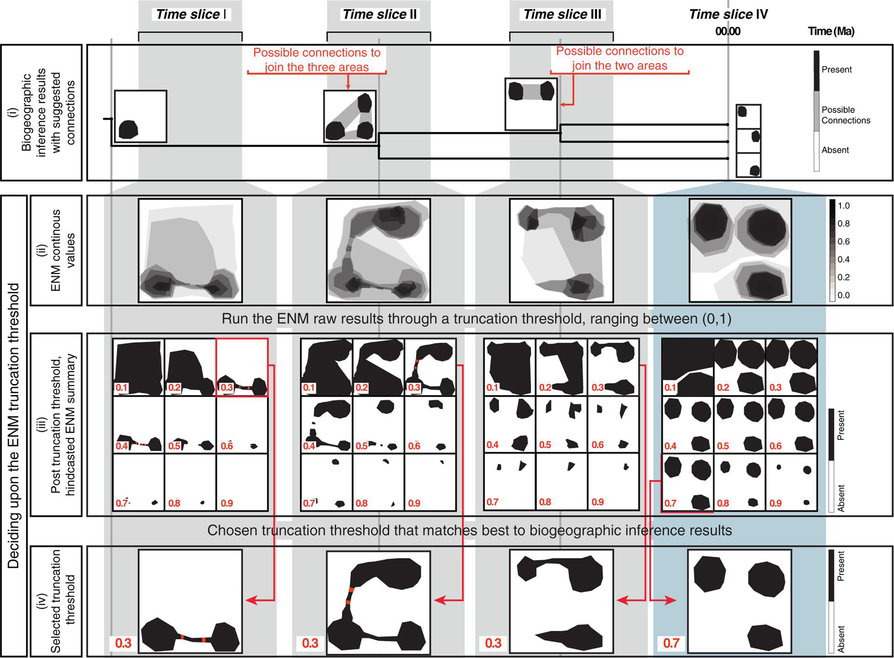
Figure 2. The biogeographically informed truncation threshold criteria to select the truncation threshold value for the ENM projections: The upper row shows three paleo-time slices I–III and one preindustrial time slice IV used in our artificial example. (i) The biogeographic inference that represents the stem-, crown-, and node ancestors of an artificial genus example (tree not to scale). Maps at tips show the current distribution of each species, maps at nodes represent the ancestral distributions inferred in the biogeographic analysis (black). For some nodes, there are suggested connections between potential distribution of ancestors (gray shading). (ii) Continuous ENM projections of the artificial genus hindcasted across the four time slices before applying the truncation threshold. (iii) The continuous ENM projections are run through different truncation thresholds values, ranging from between [0, 1]. Cells with values that fall below the truncation threshold are colored white (“absent”); those equal to or greater than the threshold are colored black (“present”). The red circles represent clusters of connected suitable cells (here, suitable cells are considered connected if the distance between them is ≤ one unsuitable cells). (iv) Chosen the truncation threshold: for hindcasted ENMs, we select the value that generates the best match the inferred ancestral distributions in the biogeographic analysis, this was 0.3 for the paleo time slices I-III in our artificial example. For the present-day time slice IV, we select truncation threshold values that generates an absence/presence map using an established truncation threshold criteria to select the truncation threshold. In this study we consider the minimized distance of the ROC curve truncation threshold criteria (MinROCdist; PresenceAbsence R Package, Freeman and Moisen, 2008), here 0.7 in our artificial example.

Hindcasted ENM Projections

To generate the past ENM predictions for both genera, we projected upon each of the four time slices the twelve ENMs built on the monthly prec-temp datasets, as well as the single ENM built on the bioclimatic dataset. As described above, the continuous value predictions from the twelve monthly prec-temp ENMs were averaged to calculate a “yearly” prec-temp ENM projection for each time slice. Lastly, we used our truncation threshold method to create post-truncation absence/presence maps for the bioclimatic ENM and the yearly prec-temp ENM projections, as described in the next section (see also Figure 2).

Spatial Correspondence Across the Hemispheres

To explore if using monthly values for ENM projections is appropriate when the genus distribution spans the northern and southern hemispheres, we performed an additional analysis with the present-day prec-temp dataset. We built monthly ENMs for both genera based on the original, non-inverted present-day datasets and projected them onto the four inverted paleo- and preindustrial world-time slices. We then used our truncation threshold to create post-truncation threshold binary maps. As above, we measured the strength of association between the non-inverted and inverted yearly ENM projections by calculating the Spearman’s rho statistic for the pre-truncation maps and the Simpson’s Similarity Index for the post-truncation projections.

Using Biogeographic Information to Select the Truncation Threshold Value

A common practice in ecological niche modeling is to truncate the continuous value predictions returned by ENM projections to produce binary absence/presence maps of habitat suitability that are more readily interpretable (Diniz-Filho et al., 2010). This truncation threshold is typically selected by using model fitting techniques and a training dataset, subsetted from the original dataset (Allouche et al., 2006; Diniz-Filho et al., 2010). The same selected truncation threshold is used across all temporal scales. Here, we propose a different truncation threshold method that uses information obtained from biogeographic inference and allows for the grouping of time slices at different temporal scales. Figure 2 demonstrates this approach using a theoretical example, a genus with three species distributed in three disjunct regions. First (Figure 2i): biogeographic analysis, based on distributional and phylogenetic data, is used to infer ancestral ranges at every node in the phylogeny, and these ranges along with current distributions are represented as absence/presence maps; if the ancestral range is composed of disjunct areas, potential connections among these areas are represented as gray shading in the maps. Second (Figure 2ii): continuous hindcasted ENM projections are generated for each time slice crossed by the phylogeny. Third (Figure 2iii): the resulting continuous ENM projections are run through alternative truncation threshold values, ranging from 0 to 1, to generate binary habitat suitability maps; grid cells with values equal to or greater than the truncation threshold are assigned the value of 1, indicating suitable climatic habitat (black cells in Figure 2iii); those lower, are assigned a value of 0, i.e., unsuitable habitat (white cells). Next, for each truncation threshold value, the resulting post-truncation ENM is examined to find clusters of connected cells with suitable habitats: suitable cells are considered connected if they are separated by no more than one unsuitable cell (red cells in Figure 2iii). Fourth (Figure 2iv): the post-truncation ENMs are compared with the nodal ancestral ranges and the tip distribution maps (i.e., the current species geographic distribution in Figure 2i); the threshold value that generates ENM projections that best match these ranges is selected as the optimal threshold value. For comparing the post-truncation ENMs projections against the tip species distribution maps, we used an established truncation threshold criterion: the minimized distance of the ROC curve, MinROCdist, as estimated in the PresenceAbsence R Package (Freeman and Moisen, 2008). This criterion implies finding the threshold value that minimizes the distance between the ROC plot and the upper left corner of the unit square, which represents the probability that the model correctly predicts the observed presences and absences. MinROCdist has been recommended as suitable for general use in the building of ENMs for extant species (Jiménez-Valverde and Lobo, 2007).

We selected a single optimal threshold value for all three paleoclimate time slices I, II, and III. The Preindustrial world time slice IV had its own optimal threshold value calculated with the MinROCdist method. Allowing for different truncation threshold criteria for the paleoclimate versus the Preindustrial time slices is justified on the different spatial scale resolution between datasets. Our paleoclimate time slices have a coarser spatial resolution than the preindustrial one (100 km vs. 1 km), and, thus, are probably less sensitive for detecting habitat suitability. Furthermore, there is increasing uncertainty in our habitat suitability predictions the further in time we project ENMs. Therefore, a higher, more conservative threshold value is needed for the Preindustrial time slice, and a lower, less restrictive threshold value for the paleoclimate time slices.

Results

Present-Day ENM Projections

Figure 3A shows the continuous post-truncation ENM projections for Camptoloma and Canarina built upon the present-day bioclimatic, full and prec-temp datasets (the latter are presented as the “yearly” monthly averaged values). Figure 3B shows the corresponding post-truncation ENM projections under the truncation threshold value selected under the MinROCdist criterion, which oscillates between a value of 0.93 and 0.99. Supplementary Table 3 reports the performance statistics (error, accuracy, and precision, etc.) for each model under the selected threshold value. All models performed well for all statistics except for precision, which was consistently low across models. In our study, precision assumes that each genus that we have recorded is present in all possible locations with a suitable habitat, which is clearly not the case. Our presence datasets for Camptoloma and Canarina are incomplete because, as mentioned in the introduction, data collection is difficult, and the genera that we are modeling have a limited geographic distribution. Supplementary Table 4 presents the statistics for the strength of association between the full-ENM and the prec-temp and bioclimatic-ENM present-day projections. In the case of the pre-truncation threshold projections, the full and prec-temp datasets showed a “strong association” (according to the descriptor in Dancey and Reidy, 2007) in Camptoloma (Spearman’s rho = 0.45), and a very strong association in Canarina (Spearman’s rho = 0.93). The pre-truncation threshold projections based on the present-day full and bioclimatic datasets showed a weak association in Camptoloma (Spearman’s rho = 0.21), but strong in Canarina (Spearman’s rho = 0.78). The Simpson’s Similarity Index showed a strong to very strong association between the post-truncation threshold present-day projections (Supplementary Table 4) based on the full dataset and the prec-temp and bioclimatic datasets, suggesting that when an appropriate truncation threshold is used, even projections with weak associations become strong. In all, these results support our contention that the monthly mean temperature and precipitation variables included in the paleoclimate datasets hold enough information to make reliable predictions about habitat suitability, and thus can be used for ENM hindcasting over the paleo and preindustrial time slices (see below).

FIGURE 3

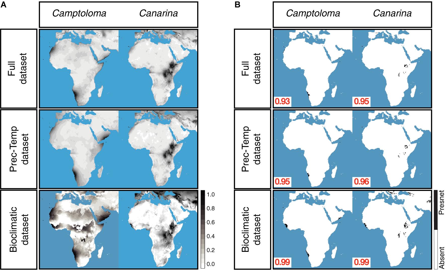
Figure 3. Preindustrial ENMs. (A) Continuous, preindustrial geographical projections of the full, bioclimatic and prec-temp ENMs for genus Camptoloma and Canarina, with the ENMs created on present-day climatic data. For the full and prec-temp ENMs, we present the “yearly” average of the month ENM projections. (B) Absence/presence maps for full, bioclimatic and prec-temp ENMs for genus Camptoloma and Canarina after applying selected truncation threshold value obtained from MinROCdist, [range = (0.93, 0.99)] to the continuous projections shown in (A). Black indicates habitat suitability and white habitat unsuitability.

Hindcasted ENM Projections

Figure 4 shows the hindcasted ENM projections, both pre-truncation (continuous) and post-truncation (presence/absence), based on the prec-temp dataset in the case of Camptoloma, and on the bioclimatic dataset in the case of Canarina and for each of the four time slices. Supplementary Figure 1 shows the post-truncation ENM projections for different threshold values in Camptoloma (Supplementary Figure 1A) and Canarina (Supplementary Figure 1B) using the same datasets as above. For the paleoclimate time slices I-III, a truncation threshold value of 0.12 was selected for Camptoloma and a value of 0.21 for Canarina. For the Preindustrial world time slice IV, a truncation threshold value of 0.95 was selected for Camptoloma and of 0.99 for Canarina. In both genera, the hindcasted ENM projections show a much larger extension of suitable habitat in the past compared to the present-day distribution. Furthermore, the paleoclimate projections predicted the existence of suitable habitat corridors connecting the currently disjunct species ranges during the Miocene and Pliocene: these involve central and northern Africa during the LMC for Canarina, and the LMC and MPWE for Camptoloma (Figure 4).

FIGURE 4

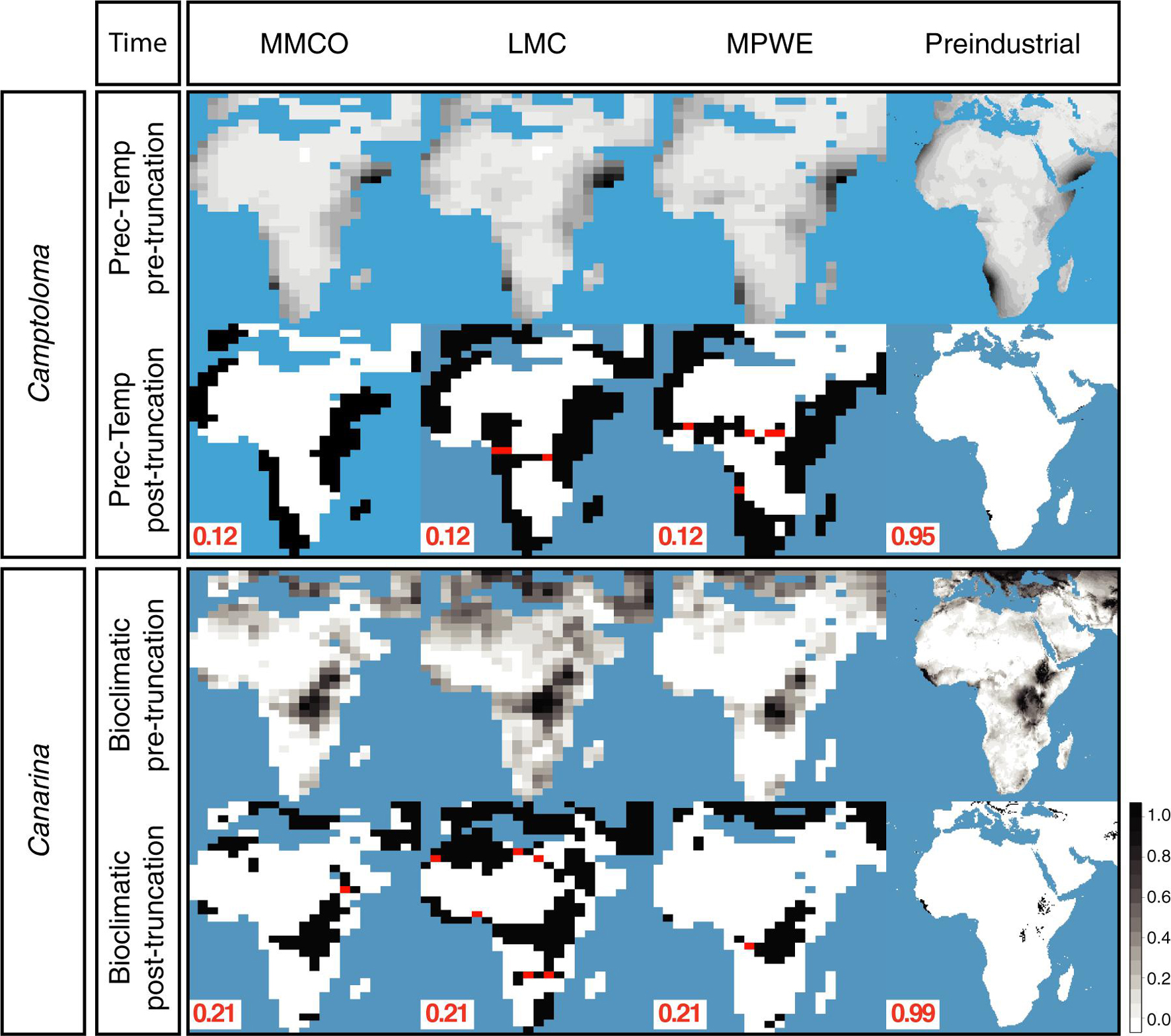
Figure 4. Hindcasted ENMs. Continuous and geographical projections for the best fitted ENMs for Camptoloma and Canarina over the four time slices: Mid Miocene Climate Optimum (MMCO, 17-14 Ma); Late Miocene Climate Cooling, (LMC, 11.6-5.3 Ma); Mid Pliocene Climate Warming (MPWE, 3.6-2.6 Ma); and preindustrial world (up to 1900). Here we selected the ENM created from the prec-temp dataset for Camptoloma and the bioclimatic dataset for Canarina. A truncation threshold of 0.12 and 0.22 was selected for Camptoloma and Canarina, respectively, for the paleo time slices, and 0.95 and 0.99 for Camptoloma and Canarina, respectively, for the preindustrial world. Black/white legend bar: “Black” indicates suitable habitat and “white” unsuitable habitat; gray scale legend bar indicates habitat suitability. Supplementary Figure 1 shows in more detail how the truncation threshold was fine-tuned across the paleo time slices.

Supplementary Figure 2 shows the post-truncation hindcasted ENM projections across different threshold values based on the alternative climatic dataset for each genus, that is, ENM projections for the bioclimatic dataset in Camptoloma (Supplementary Figure 2A) and ENM predictions based on the yearly prec-temp dataset in Canarina (Supplementary Figure 2B). Comparisons indicated that for ENM projections based on these particular datasets and genera, it was not possible to find an optimal threshold value across the three paleoclimate time slices. Therefore, the bioclimatic and prec-temp ENMs for Camptoloma and Canarina, respectively, were excluded from further analysis. Finally, Figure 5 demonstrates the need to use a different truncation threshold value for different temporal scales: we compared post-truncation ENM projections for the three paleoclimate time slices I-III that were generated using either the threshold value for the Preindustrial time slice IV, calculated with the minimized distance ROC curve, versus the post-truncation ENM projections for the three paleoclimate time slices I-III that were generated using an independent threshold value calculated with the biogeographically informed truncation method described in Figure 2. Results, shown here for Camptoloma prec-temp and Canarina bioclimatic ENMs, respectively, indicate that using the MinROCdist method is too restrictive and fails to recover any spatial distribution pattern in the ENM hindcasts of the paleoclimate time slices I-III that fits the biogeographic inference results.

FIGURE 5

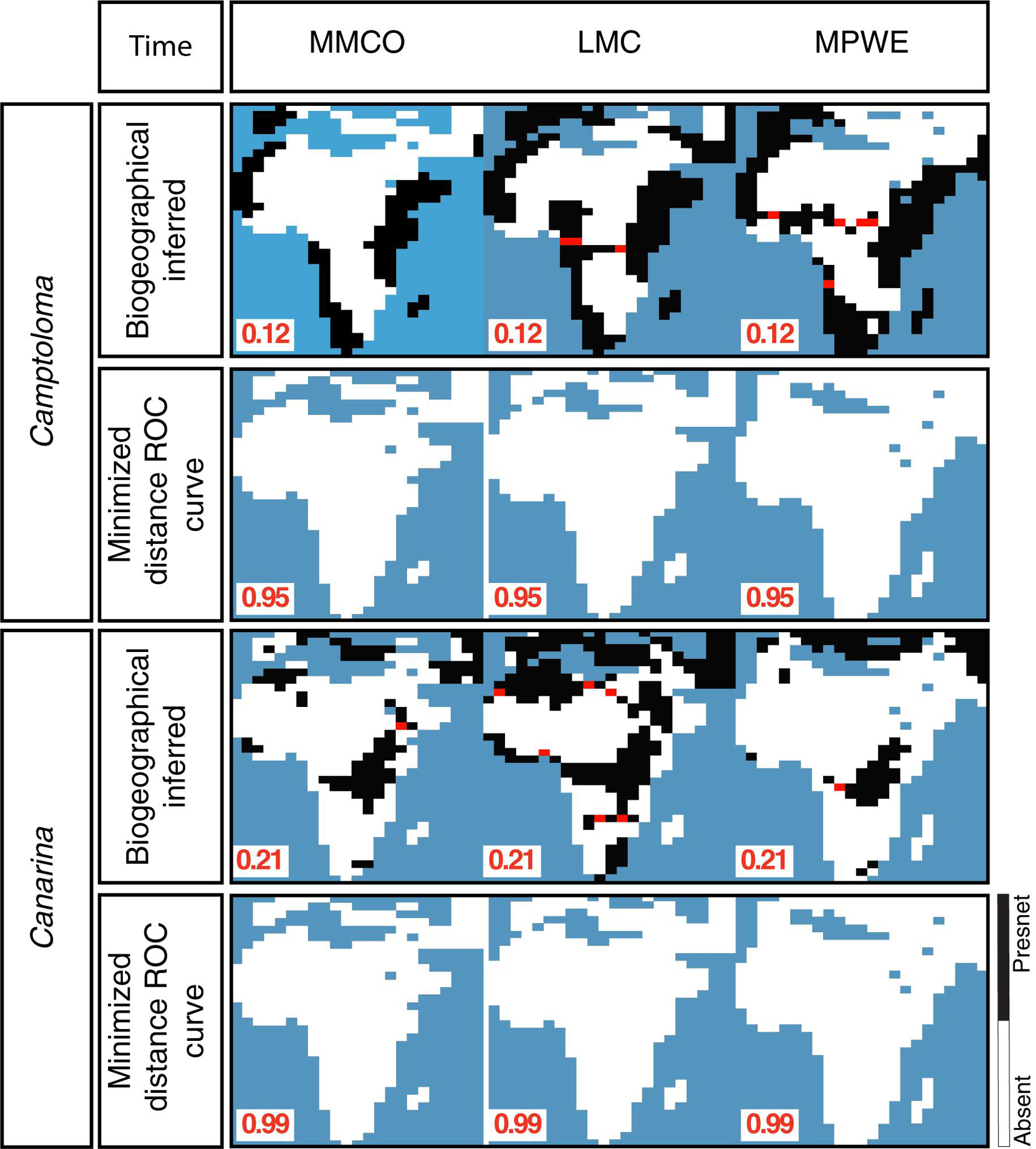
Figure 5. Performance comparison between the biogeographically-informed truncation threshold criterion and minimized distance ROC curve truncation threshold criteria.

Spatial Correspondence Between Hemispheres

Supplementary Figure 3 and Supplementary Table 4 show the results of the comparison between the pre- (Supplementary Figure 3A) and post-truncation (Supplementary Figure 3B) ENMs generated with the non-inverted versus the inverted prec-temp dataset for Camptoloma (we did not investigate hemisphere effects in Canarina, since, as explained above, the prec-temp ENMs for this genus were excluded from further analyses). The truncation threshold value for the non-inverted prec-temp ENM projections was 0.97 for the preindustrial time slice and 0.1 for the paleoclimate time slices. A very strong association between the non-inverted and inverted prec-temp ENM projections was found for each of the four time slices [pre-truncation threshold: Spearman’s rho range = [0.72, 0.83]; post-truncation threshold: Simpson’s Similarity Index range = (0.78, 0.88)]. Moreover, the non-inverted and inverted post-truncation threshold ENM maps showed a similar history of range shift events, with climatic corridors in the LMC and MPWE time slices connecting the currently disjunct species distributions. This suggests that the hemisphere effect did not bias our yearly monthly averaged ENM projections in Camptoloma, and therefore had no effect in our predictions.

Reconstructing Geographic Range Shifts Using ENM Projections and Biogeographic Inference

Figure 6iii reconstructs the history of geographic range shifts in Camptoloma and Canarina using information provided by the biogeographic inference analysis (Figure 6i) and the hindcasted ENM projections (Figure 6iii). The inferred ancestral ranges in Camptoloma (Figure 6Ai) matched the climatically suitable areas depicted in the post-truncation ENM projections based on the prec-temp dataset (Figure 6Aii). In Canarina, the hindcasted ENMs based on the bioclimatic dataset (Figure 6Bii) also showed a good match to the biogeographic inferences (Figure 6Bi).

FIGURE 6

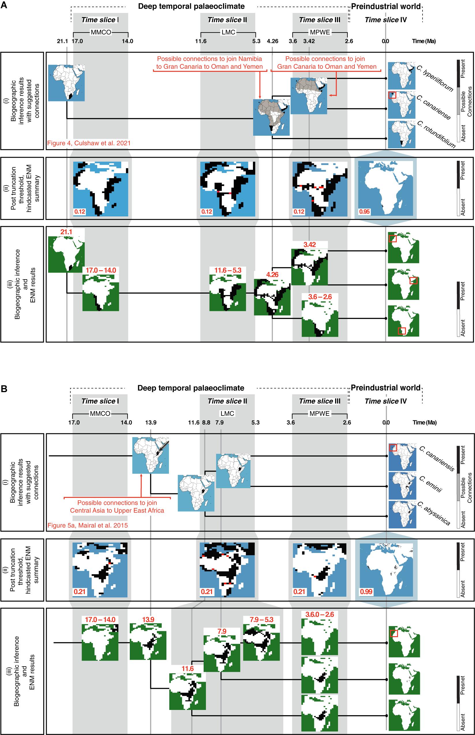
Figure 6. Combining information from biogeographic inference and ENM to reconstruct the spatio-temporal evolution of (A) Camptoloma and (B) Canarina: The upper rows show three paleoclimate-time slices (I–III) and preindustrial time slice (IV). (i) A summary of the biogeographic inference depicting the species current distribution and inferred ancestral distributions at nodes (tree not to scale; for more details for (A) see Figure 4 in Culshaw et al., 2021 and (B) Figure 5A in Mairal et al., 2015). (ii) The selected truncation thresholds for hindcasted ENMs (see Figure 2 for more details). (iii) The post-truncation threshold ENM maps are cleaned up by removing presence locations that do not match those from the biogeographic inference. Then, results provided by the ENMs are used together with those from the biogeographic inference to infer a detailed history of the spatiotemporal evolution or each genus. For Camptoloma (A) we represent the “yearly” prec-temp ENM projections with a truncation threshold of 0.12 for the paleoclimate-time slice projections and 0.95 for the Preindustrial world time slice projection for Canarina (B) we represent the bioclimatic ENM projections with a truncation threshold of 0.22 for the paleoclimate-time slice projections and 0.99 for the Preindustrial world time slice projection.

Discussion

ENMs and Biogeographic Inference Used in Tandem Reconstruct Geographic Range Shifts in Rare Endemics

In the original studies exploring Canarina and Camptoloma biogeographic history (Mairal et al., 2015; Culshaw et al., 2021), the currently disjunct distribution of the extant species was explained by ecological vicariance and climate-driven extinction linked to Neogene aridification cycles, in agreement with other Rand Flora lineages (Pokorny et al., 2015; Rincón-Barrado et al., 2021). However, the small phylogenies, with only three species each, and the deep evolutionary divergences, introduced large uncertainty in ancestral range inference; for example, the Western Asian origin of Canarina (Mairal et al., 2015) or the southern African stem-ancestor of Camptoloma (Culshaw et al., 2021), were associated with marginal probabilities lower than 0.1.

In our study, the introduction of additional information provided by hindcasted ENM projections was able to clarify some of these uncertain biogeographic inferences, in particular along the long internodal branches. For example, ENM projections support a restricted distribution of stem-Camptoloma, in southwestern Africa in the Early-Mid Miocene (21 Ma), while the crown-ancestor is reconstructed as occupying eastern Africa-southern Arabia and Macaronesia already in the Early Pliocene (4.6 Ma, Figure 6Aii). ENM projections (Figure 6Aii) support also the hypothesis of a northeastward dispersal of the ancestor of Camptoloma during the 15-million year branch length separating the stem and crown nodes (Figure 6Aiii, Culshaw et al., 2021): the ENM predictions for time slices I and II showed the presence of suitable habitat corridors over central-eastern Africa during the MMCO (17-14 Ma) and the LMC (12-5 Ma) time slices (Figure 6Aiii). Similarly, the biogeographic inference of a widespread distribution across northern Africa for the most recent common ancestor of Camptoloma canariense and C. lyperiiflorum (3.4 Ma, Figure 6Ai), Culshaw et al., 2021) is supported by the ENM projection for time slice III, which shows climatic corridors with suitable habitat during the MPWE (Figure 6Aii); these disappear in the preindustrial projection (Figure 6Aiii).

Mairal et al. (2015) inferred a stem-ancestor of Canarina distributed in central Asia around the Mid Miocene (13.9 Ma, Figure 6Bi), which migrated to eastern Africa during the Mid-Late Miocene (11-8 Ma). This scenario is supported by our hindcasted ENM projections (Figure 6Bii), which show suitable habitat in western Asia and central-eastern Africa during the MMCO interval. The ca. 8 million-year branch separating the disjunct sister species C. canariensis and C. eminii was explained in Mairal et al. (2015) by short-range dispersal over climatic corridors across the Sahara during the Late Miocene, followed by climatic extinction in the Pliocene (Figure 6Bi). The ENM projections for time slices II and III support these inferences, depicting corridors of suitable habitat across the Sahara during the wetter and colder climates of the LMC (Figure 6Bii), which disappear in the projections of the drier MPWE (Figure 6Bi).

Using Biogeographical Inference as Truncation Threshold Criteria in ENMs

A known difficulty in building ENMs for rare endemics is the selection of the optimal truncation threshold value (Diniz-Filho et al., 2010). The selection of a threshold value often relies upon model fit tests, such as the Kappa statistic (Monserud and Leemans, 1992; Fielding and Bell, 1997), the true skill statistic (TSS, Allouche et al., 2006), or the Receiver Operator Characteristic (ROC). All of these approaches rely on using a training dataset, subsetted from the original data, and evaluating model fit through examination of true and false predictions of species presences and absences (Liu et al., 2005; Jiménez-Valverde and Lobo, 2007). When the georeferenced data is complete and unbiased, and the ENMs are hindcasted upon shallow timescales, these truncation threshold criteria are reliable. However, when occurrence records are incomplete or biased toward certain regions, or when ENMs are hindcasted upon deep timescales, as in our study, these methods can lead to biased habitat suitability projections, as demonstrated in Figure 5.

Here, we propose an alternative approach that uses ancestral nodal ranges inferred through biogeographic inference as an independent source of information for selecting the truncation threshold value of ENM projections (Figure 2). Our approach is particularly suited for ENMs hindcasted into the distant past, where traditional criteria such as the MinROCdist result in very restrictive and conservative truncation threshold values and fail to recover any spatial pattern (Figure 5). Our study, thus, supports the importance of using an appropriate truncation threshold criterion when using absence/presence ENM models (Nenzén and Araújo, 2011), especially when comparing paleoclimate vs. predindustrial hindcasted projections.

The Importance of Temporal Resolution When Building ENMs

There has been recent discussion on the importance of including fine-scale temporal resolution in the environmental data used for building ENMs (Kearney et al., 2012; Gardner et al., 2020; Perez-Navarro et al., 2020). The average-year bioclimatic variables obtained from WorldClim might be too coarse in temporal resolution to capture the climatic niche of short-lived species or species with large geographic ranges and contrasting seasonal regimes, for example, those distributed north and south of the equator (Kearney et al., 2012; Montalto et al., 2014). The importance of considering temporal resolution in climatic data has been emphasized also for paleoclimate data. Even if WorldClim bioclimatic variables correlate with physiological predictors, these relationships could break down when results are extrapolated into other time frames (Elith and Leathwick, 2009). Bova et al. (2021) recently showed that the mismatch between paleoclimate simulations and temperature reconstructions from geological records disappear when seasonal variation over time is employed instead of long-term averages.

In the case of Camptoloma, ENM projections built on the yearly averaged, monthly variables of the prec-temp dataset showed a strong association to those built on the full climatic dataset (Supplementary Table 4), suggesting that monthly mean temperature and precipitation contained enough information to infer ancestral tolerances when projected into the past; in contrast, ENMs built on the annual variables of the bioclimate dataset showed a weak association and we could not find an optimal threshold value for hindcasted projections (Supplementary Table 4 and Supplementary Figure 2). For Canarina, the opposite pattern was found: the ENM projections built on the annual bioclimatic variables showed a strong association with the full dataset, while the monthly averaged prec-temp projections proved to be less informative (Supplementary Table 4 and Supplementary Figure 2). These differences between the two genera may be explained by their different “rarity” character. Camptoloma fits Rabinowitz’s (1981) definition of a “narrow rare endemic”: a rare species with small populations restricted to climatic microrefugia. Camptoloma rotundifolium occurs in moist escarpments in the Namibian Brandberg Mountains, whereas C. canariense grows in shaded vertical crevices on the coastal slopes and cliffs of Gran Canaria and C. lyperiiflorum inhabits a special wetter microclimate in Socotra Island (Culshaw et al., 2021). In contrast, Canarina fits the definition of a “widespread rare endemic” (Rabinowitz, 1981): Canarina canariensis occurs in five of the seven Canary Islands, while the geographic range of C. eminii extends from Ethiopia in the north to Malawi in the south (Mairal et al., 2018). Moreover, Canarina species can spend unfavorable seasons throughout the year in a tuber/root form, which could buffer the influence of climate extreme events on species’ survival, growth and reproductive capacity (Hedberg, 1961). It might be that the use of fine-temporal resolution environmental data, i.e., the yearly averaged monthly values from the prec-temp dataset, is important for modeling the climatic preferences of a species with restricted habitats and little capacity for behavioral buffering, such as Camptoloma, whereas the annual bioclimatic variables from WorldClim work well for the more widespread Canarina. Our study thus supports the hypothesis that temporal resolution of environmental data when building ENMs should be at a scale adequate to understand physiological responses to climate change in the organism under study (Gardner et al., 2020), or in other words, at a scale over which biological responses directly influence their predicted presences in ENM models (Montalto et al., 2014).

Conclusion

We showed that combining information provided by hindcasted ecological niche models and phylogenetic biogeographic inference can be useful in reconstructing geographic range shifts that resulted from climate change, as found in rare endemics with sparse and biased sampling and ancient origins. Biogeographic inference can be used to select the truncation threshold value to build ENM presence/absence maps for the distant past, whereas hindcasted ENMs can inform biogeographic inference over phylogenetic intervals with no observable diversification events. We additionally demonstrate the importance of temporal resolution in ENMs, especially in narrow rare endemics characterized by limited sampling and with restricted physiological requirements.

Data Availability Statement

The original contributions presented in the study are included in the article/Supplementary Material, further inquiries can be directed to the corresponding authors. Code to run analyses is provided in the GitHub repository: github.com/vickycul.

Author Contributions

VC and IS designed the study. MM and VC collected and sourced samples. VC analyzed the data with help from IS. IS and VC wrote the manuscript, with contributions from MM. All authors contributed to the article and approved the submitted version.

Conflict of Interest

The authors declare that the research was conducted in the absence of any commercial or financial relationships that could be construed as a potential conflict of interest.

Publisher’s Note

All claims expressed in this article are solely those of the authors and do not necessarily represent those of their affiliated organizations, or those of the publisher, the editors and the reviewers. Any product that may be evaluated in this article, or claim that may be made by its manufacturer, is not guaranteed or endorsed by the publisher.

Funding

VC was funded by Fellowship (BES-2013-065389) from the Spanish Ministry of Economy and Competitiveness (MINECO) and supervised by IS. IS was funded by grant CGL2015-67849-P from MINECO and the European Regional Development Fund (FEDER).

Supplementary Material

The Supplementary Material for this article can be found online at: https://www.frontiersin.org/articles/10.3389/fevo.2021.662092/full#supplementary-material

Supplementary Figure 1 | Demonstrating how to select a suitable truncation threshold with the biogeographically-informed truncation threshold criterion for (A) the Camptoloma prec-temp ENM paleo projections and (B) the Canarina bioclimatic ENM paleo projections. Black indicates presence, white indicates absence, and red represents the bridge between black cells that are no more than one white cell apart (see Figure 2 for more details). The biogeographic inference results that were used as the criterion to select the truncation threshold can be seen in Figure 6i.

Supplementary Figure 2 | Demonstrating the inability to find a suitable truncation threshold with the biogeographically-informed truncation threshold criterion for (A) the Camptoloma bioclimatic ENM paleo projections and for (B) the Canarina prec-temp ENM paleo projections. Black indicates presence, white indicates absence, and red represents the bridge between black cells that are no more than one white cell value apart (see Figure 2 for more details). It can be seen that regardless of the threshold, most of the binary maps resemble one another, and more importantly they do not represent the biogeographic inference results (seen in Figure 6i) that are used as a criterion for the selection of the truncation threshold. For example, in Camptoloma, the bioclimatic models (Supplementary Figure 2A) predict high habitat suitability across the Sahara Desert in the MMCO and LMC layers; in Canarina, the prec-temp dataset (Supplementary Figure 2B) does not show connections across northern Africa in the LMC time slice, as expected from the biogeographic results.

Supplementary Figure 3 | Exploring if the “hemisphere” effect introduces a bias into the Camptoloma binary ENM hindcast projections for the prec-temp dataset, where each projection is a “yearly” average of the month ENMs results. The ENM prec-temp projections for the non-inverted and inverted binary maps have similar truncation thresholds (0.1 vs. 0.12) and both show absence/presence distributions for each time slice.

Supplementary Table 1 | Climatic variables from WorldClim2 (Fick and Hijmans, 2017) with acronyms and units used in the study.

Supplementary Table 2 | Variables per month that were retained after the full present-day climatic dataset was run through correlation matrices. Only variables with low absolute correlated attributes (correlation lower than 0.75) were included in the final models.

Supplementary Table 3 | ENM performance statistics at selected present-day truncation threshold for genera Camptoloma and Canarina.

Supplementary Table 4 | The strength of association among the three present-day maps calculated as the Spearman’s rho statistic for the pre-truncation threshold projections and the Simpson’s Similarity Index for the post-truncation threshold projections.

Supplementary Appendix 1 | The geographic occurrence and climatic data used for ecological niche modeling in Camptoloma and Canarina. This data has been normalized to lie within the closed boundaries [0, 1], and the hemispheres were “inverted” (details in section “Materials and Methods”) to account for the “hemisphere effect.”

Footnotes

References

Allouche, O., Tsoar, A., and Kadmon, R. (2006). Assessing the accuracy of species distribution models: prevalence, kappa and the true skill statistic (TSS). J. Appl. Ecol. 43, 1223–1232. doi: 10.1111/j.1365-2664.2006.01214.x