 Laura H. Antão
- 1Centre for Biological Diversity, University of St Andrews, St Andrews, United Kingdom
- 2Department of Biology and CESAM, Universidade de Aveiro, Aveiro, Portugal
- 3Organismal and Evolutionary Biology Research Programme, Research Centre for Ecological Change, University of Helsinki, Helsinki, Finland
Species abundance distributions (SADs) describe community structure and are a key component of biodiversity theory and research. Although different distributions have been proposed to represent SADs at different scales, a systematic empirical assessment of how SAD shape varies across wide scale gradients is lacking. Here, we examined 11 empirical large-scale datasets for a wide range of taxa and used maximum likelihood methods to compare the fit of the logseries, lognormal, and multimodal (i.e., with multiple modes of abundance) models to SADs across a scale gradient spanning several orders of magnitude. Overall, there was a higher prevalence of multimodality for larger spatial extents, whereas the logseries was exclusively selected as best fit for smaller areas. For many communities the shape of the SAD at the largest spatial extent (either lognormal or multimodal) was conserved across the scale gradient, despite steep declines in area and taxonomic diversity sampled. Additionally, SAD shape was affected by species richness, but we did not detect a systematic effect of the total number of individuals. Our results reveal clear departures from the predictions of two major macroecological theories of biodiversity for SAD shape. Specifically, neither the Neutral Theory of Biodiversity (NTB) nor the Maximum Entropy Theory of Ecology (METE) are able to accommodate the variability in SAD shape we encountered. This is highlighted by the inadequacy of the logseries distribution at larger scales, contrary to predictions of the NTB, and by departures from METE expectation across scales. Importantly, neither theory accounts for multiple modes in SADs. We suggest our results are underpinned by both inter- and intraspecific spatial aggregation patterns, highlighting the importance of spatial distributions as determinants of biodiversity patterns. Critical developments for macroecological biodiversity theories remain in incorporating the effect of spatial scale, ecological heterogeneity and spatial aggregation patterns in determining SAD shape.
Introduction
Species Abundance Distributions (SADs) describe the relative abundance of the species within a community. Looking at the whole distribution allows accounting for different aspects that univariate metrics measure separately and readily integrating concepts such as rarity and dominance (Magurran, 2004; McGill et al., 2007). SADs are thus a synthetic measure of biodiversity and community structure, and a key component of biodiversity theory and research. The two most common distributions used to describe SADs are the logseries (Fisher et al., 1943) and the lognormal (Preston, 1948). These distributions differ mainly in the proportion of rare species they predict; specifically, the logseries has no internal mode, with singletons as the modal class, whereas an unveiled lognormal has one internal mode for species with intermediate abundances (Fisher et al., 1943; Preston, 1948). Additionally, multimodal SADs, i.e., with more than one mode of abundance can also occur (Gray et al., 2006; Dornelas and Connolly, 2008). While this pattern had been mostly disregarded, a recent empirical meta-analysis showed that not only is multimodality more common than previously recognized, it is also more likely to occur for communities encompassing larger spatial extents or with higher taxonomic diversity (Antão et al., 2017). Despite decades of research, multiple hypotheses and theories proposed to explain SADs, a thorough understanding of what drives SAD shape is still lacking (Hubbell, 2001; Connolly et al., 2005; Green and Plotkin, 2007; McGill et al., 2007); this gap is particularly apparent for large spatial scales (Enquist et al., 2019; Fukaya et al., 2020). A systematic empirical assessment of how SAD shape varies with scale is needed to improve our understanding of the mechanisms underpinning SAD shape, and consequently community structure. Given the pivotal role of SADs in biodiversity research, these insights will further facilitate assessments of ongoing biodiversity change.
Understanding how SAD shape varies with sampling scale is a long standing question in ecology (Fisher et al., 1943; Preston, 1948; McGill et al., 2007; Zillio and He, 2010). Both sampling effects and spatial scale are known to affect SAD shape (Fisher et al., 1943; Preston, 1948; Pielou, 1977; Hubbell, 2001; Connolly et al., 2005; Green and Plotkin, 2007). Two approaches to understanding the scaling properties of SADs can be used: downscaling—i.e., try to predict the shape of SADs at smaller scales from the regional scale (e.g., Hubbell, 2001; Green and Plotkin, 2007), and upscaling—i.e., try to infer the SAD for larger spatial scales by pooling smaller scale SADs (Šizling et al., 2009b; Zillio and He, 2010; Borda-de-Água et al., 2012). However, analyzing SADs across different spatial scales has remained largely unexplored (but see Rosindell and Cornell, 2013). As there is no single ideal scale for studying SADs (Wiens, 1989; Levin, 1992), systematically assessing SADs along spatial scale gradients allows us to make stronger inferences about patterns of commonness and rarity across scales, and can potentially provide insights to help disentangle which processes are relevant at different scales.
Generally, SAD studies have relied on sampling theory approaches to address the relationship between the large regional community and local scale SADs. For instance, Fisher et al. (1943) viewed the logseries as resulting from a random sample from a gamma distribution (i.e., SADs at smaller scales are random subsamples of SADs at larger scales). The “veil line” proposed by Preston (1948) was a first attempt to explain that the absence of rare species in small samples would lead to a truncation of the “true” underlying lognormal distribution, which would gradually disappear with increasing sampling. The lognormal has since been a particularly prominent SAD model, emerging as the statistical expectation of the Central Limit Theorem (i.e., SADs result from random multiplicative processes acting on species abundances), and from population dynamics and niche partitioning models (Preston, 1948; May, 1975; Magurran, 2004; McGill et al., 2007). However, unveiling does not simply reveal the left-end of the distribution by rigidly moving the veil, but the shape of the overall distribution also changes (Pielou, 1977; Dewdney, 1998; McGill, 2003b), which can affect the overall proportion of the rarest species. For instance, McGill (2003b) showed that pooling repeated autocorrelated small samples can lead to the log-left-skew reported in many empirical SADs, i.e., the existence of more rare species than predicted by a lognormal distribution (Hubbell, 2001). This phenomenon can nonetheless be driven by biological mechanisms, where SAD shape reflects changes in community structure, such as the signature of core-transient species temporal dynamics (Magurran and Henderson, 2003).
Crucially, SAD shape is affected by how species are distributed in space. One of the fundamental patterns in ecology is that individuals are not randomly distributed in space (Condit et al., 2000; McGill, 2010), with both theoretical and empirical studies evaluating these effects. Spatial aggregation patterns and turnover affect SAD shape when upscaling from smaller areas (Šizling et al., 2009a). Green and Plotkin (2007) developed a statistical sampling theory for SAD incorporating conspecific spatial aggregation patterns. They showed that when sampling from regional SADs with randomly distributed populations (i.e., Poisson sampling), the sampled SADs would exhibit the same functional form as the regional SAD. In contrast, using a more realistic description of species spatial aggregation patterns (i.e., negative binomial sampling), sampled SADs diverged from the regional SAD. Specifically, this conspecific spatial aggregation led to sampled SADs skewed toward both rare and more abundant species (Green and Plotkin, 2007). Interspecific differences in aggregation rates were also suggested to produce bimodal abundance distributions (Alonso et al., 2008), which in turn partially explain the existence of multiple modes (two, but not the three modes) in a coral SAD (Dornelas and Connolly, 2008). Subsequently, and taking a completely different approach while attempting to upscale SADs, Borda-de-Água et al. (2012) similarly predicted a bimodal SAD for larger scales without including any information on species aggregation patterns. In this case, bimodality arises from an increase in the number of rare species with area (Borda-de-Água et al., 2002, 2012), with one mode occurring for the singletons class and another mode for intermediate abundance classes.
Two unified theories of biodiversity in particular make explicit predictions for SAD shape at different scales—the Neutral Theory of Biodiversity (NTB; Hubbell, 2001) and the Maximum Entropy Theory of Ecology (METE; Harte et al., 2008). Both theoretical frameworks can be thought of as null models, as they assume demographic equivalence between individuals (NTB), or do not include explicit ecological mechanisms (METE). While not the only theories of SADs, both provide null expectations for what SAD shape should emerge at different scales. Systematic discrepancies between empirical data and theoretical predictions can help identify important mechanisms that need to be accounted if we are to improve our ability to make stronger inferences about the processes driving SAD shape. Below, we provide only a brief outline of both theories’ assumptions relevant for our analysis, given the extensive literature devoted to them.
NTB assumes all individuals in an assemblage have equal demographic rates of birth, death, dispersal and speciation, irrespective of species identity (Hubbell, 2001), with stochastic drift and dispersal limitation as the processes explaining patterns of species occurrence and abundance. The spatially implicit NTB model includes two distinct spatial scales: a local community that consists of a dispersal-limited sample, and the metacommunity (larger scale) from which this sample is taken. In the original model, the metacommunity follows a logseries distribution and the local community follows a zero-sum multinomial distribution (ZSM), which includes fewer rare species than the logseries and resembles a left-skewed lognormal distribution (Hubbell, 2001; Rosindell et al., 2011). This latter distribution is controversial, with numerous studies comparing ZSM and lognormal performances on fitting empirical SADs (Hubbell, 2001; McGill, 2003a; Volkov et al., 2003, 2007; Dornelas et al., 2006). Subsequent model developments also yield a logseries SAD for the largest scale [e.g., spatially explicit model (Rosindell and Cornell, 2013); protracted speciation mode (Rosindell et al., 2010)].
METE is a spatially explicit theory of biodiversity based on the principle of maximization of information entropy (MaxEnt). METE only requires knowledge on four state variables to describe ecological communities: the area of an ecosystem, species richness, the total number of individuals, and total metabolic rate (the latter has been disregarded when analyzing SADs; Harte et al., 2008; Harte and Newman, 2014). MaxEnt rationale is that the least-biased inference of the shape of a probability distribution is as smooth and flat as possible, given the constraints (Harte et al., 2008). Using only these four state variables and without incorporating any specific ecological mechanisms, the most likely distributions for several macroecological patterns are found by maximizing information entropy. The logseries is the SAD distribution that emerges across spatial scales (Harte et al., 2008; Harte and Newman, 2014). Therefore, assessing the performance of the logseries for large scale SADs, as well as for different taxa, provides a relevant test both on current neutral models and a critical assessment of METE’s expectation of a scale-independent SAD. On the other hand, neither theory accounts for multimodal SADs.
Here, we systematically assessed empirical SADs shape across a gradient in spatial scale spanning several orders of magnitude and for different taxonomic groups spanning both marine and terrestrial realms. We assessed the effect of sampled area, taxonomic diversity (species and family richness) and total abundance on SAD shape. We aimed to compare predictions for SAD shape from macroecological theories, with sampling theory predictions and empirical patterns. Specifically, we contrasted expectations of a better fit of the logseries as outlined above following NTB or METE predictions (either for larger scales or invariant with scale, respectively) (1), with the expected better performance of lognormal distributions for larger samples (2), and further with recent empirical results showing that multimodality occurs with higher prevalence for larger areas or more diverse communities (3).
Materials and Methods
Empirical Data
We analyzed 11 datasets sampled over large extents for different taxa, namely trees, birds, fish and benthos (Table 1). We selected datasets from the BioTIME database (Dornelas et al., 2018) with spatial extent larger than 150,000 km2 and for which the unique sampling locations were distributed across the study area so that the random splitting of the total extent would not result in portions without sampling locations (see below). Importantly, for all these datasets, samples were consistently collected using standardized methods (e.g., plots, transects or tows), where each sample consists of records of species and their abundance in a given time and location (more information can be found in each dataset’s original metadata, or from the BioTIME database). For each dataset, we used data corresponding to one year of sampling only, selecting the year with the most and more evenly distributed sampling locations. We further analyzed the Forest Inventory and Analysis Database (FIA; USDA Forest Service, 2010; Woudenberg et al., 2010)1, as we wanted to include a tree community data in our analysis to ensure the results are robust across a broad range of taxonomic groups. We obtained the latter data via the EcoData Retriever (Morris and White, 2013; McGlinn and White, 2015)2, and selected data from 2013 only. For each dataset, information of the taxonomic family corresponding to each species was retrieved. These empirical datasets cover a wide range of sampling grains (0.0001 to 25.4 km2) and total spatial extents (167,455 to 16,663,141 km2).
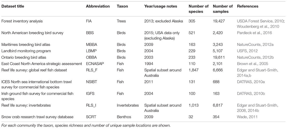
Table 1. Community data used and data sources.
Implementing the Scale Gradient
All analyses were performed in the statistical software R (R Core Team, 2017). We established a scale gradient by using the fixed extent of the study area of each dataset and systematically partitioning this area into smaller portions as follows. We drew a circle encompassing all the sampling locations from each dataset and centered on the centroid of the sampling locations. A random point from the circle was selected to split the circle into halves, thirds, quarters, eights and sixteenths, using the initial random point from the bisection as reference (Figure 1). This process ensures the spatial relationship between the sections and the sampling locations is maintained. Further details on implementing the scale gradient can be found in Antão et al. (2019). Within each section, species abundances were pooled across all the individual samples to build the species abundance distributions. Thus, one SAD was calculated for the total extent (i.e., the largest level in our scale gradient), two SADs for the bisection level, three for the third level, and so forth. At each level, each section was annotated with the area, species richness (S), total abundance (N), and total number of families, to assess the effect of taxonomic diversity on SAD shape. The areas sampled were calculated using convex hull polygons encompassing the sampling locations within each section, using package rgeos (Bivand and Rundel, 2016; Figure 1).
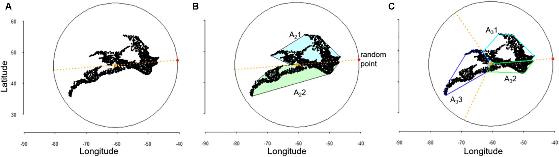
Figure 1. Schematic representation of the scale gradient, showing an example of how the encompassing circle was drawn to include all the sampling locations and a random point was selected to establish bisections (A,B) and thirds (C).
Model Fitting and Analysis
Along the scale gradient and for each section, each SAD was fitted with four alternative models, following the method implemented in Antão et al. (2017). Specifically, we employed maximum likelihood methods to explicitly compare the fit of logseries distributions (Fisher et al., 1943) and of mixtures of 1, 2, and 3 Poisson Lognormal distributions (1PLN, 2PLN, and 3PLN, respectively), where 2PLN and 3PLN are multimodal distributions (Pielou, 1969; Bulmer, 1974). We did not include the ZSM distribution in our comparisons, since our aim was to evaluate changes in SADs overall shape, rather than explicitly test NTB models or focus on detailed comparisons between alternative models fitting. This is further justified given: (1) the plethora neutral models, implementations and assumptions, without a clear way forward (Hubbell, 2001; McGill, 2003b; Etienne, 2005, 2007, 2009; Dornelas et al., 2006; Rosindell et al., 2011), (2) PLN mixtures can provide suitable alternatives to ZSM (Gray et al., 2005), and (3) ZSM is usually associated with scales overall much smaller than the lowest levels in our scale gradient. For each model above, best-fit parameters were found by minimizing the negative log-likelihood; parameter estimation was performed using the optimization routine nlminb(), with searches initialized from multiple starting points due to the possibility of several local maxima for more complex distributions (Dornelas and Connolly, 2008; Antão et al., 2017). All the fitting routines were run on non-binned data, and we only binned data for plotting purposes—SADs are traditionally plotted as histograms of the number of species as a function of abundance on a log2 scale, conveying the intuitive approach of doubling classes of abundance, called octaves (Preston, 1948; Gray et al., 2006). The second order Akaike’s information criterion for small sample sizes (AICc, Burnham and Anderson, 2002) was used for model selection. AICc was used throughout as it converges to AIC when the sample size is large (Burnham and Anderson, 2002), and previous work with simulated communities testing this PLN-mixture method has shown that BIC is too conservative and can be insensitive to deviations in SAD shape (Antão et al., 2017). Furthermore, because we were not interested in detecting multimodality per se, but rather in detecting changes in SAD shape, we assumed the best model to be the one selected by AICc, regardless of support level. We plotted smoothed density estimates of the model selected for each section as a function of the relevant variables across the scale gradient, i.e., sampling level, area sampled, species richness, total abundance and number of families, using the package ggplot2 (Wickham, 2009). These assessments were built for each community individually and for all the SADs together to provide an overview of how these variables affect SAD shape across the different datasets analyzed. In addition to using AICc as a model selection criterion, we quantified the deviations between the empirical SADs and the predictions of each model, by comparing the observed and expected number of species per octave.
Results
We built 374 SADs, which included 4,684 species and over 142.5 million individuals. Overall, there was a higher prevalence of multimodal SADs for larger areas and for more taxonomically diverse datasets (Figures 2, 3 and Supplementary Figure 1), although some smaller areas or less diverse communities were also selected as multimodal. The logseries was never selected as best model for the total extent SADs, and was only selected for much smaller areas, and when species richness or number of families were proportionally much smaller (Figures 2, 3). That is, only 1PLN, 2PLN, or 3PLN provided adequate fit for the total extent SADs, with a better performance for multimodal models. As area sampled decreases, both species richness and total number of individuals are also expected to decrease. However, while species richness showed a similar effect to that of area on model selection, there was no clear pattern for total number of individuals across the datasets analyzed (Figure 3).
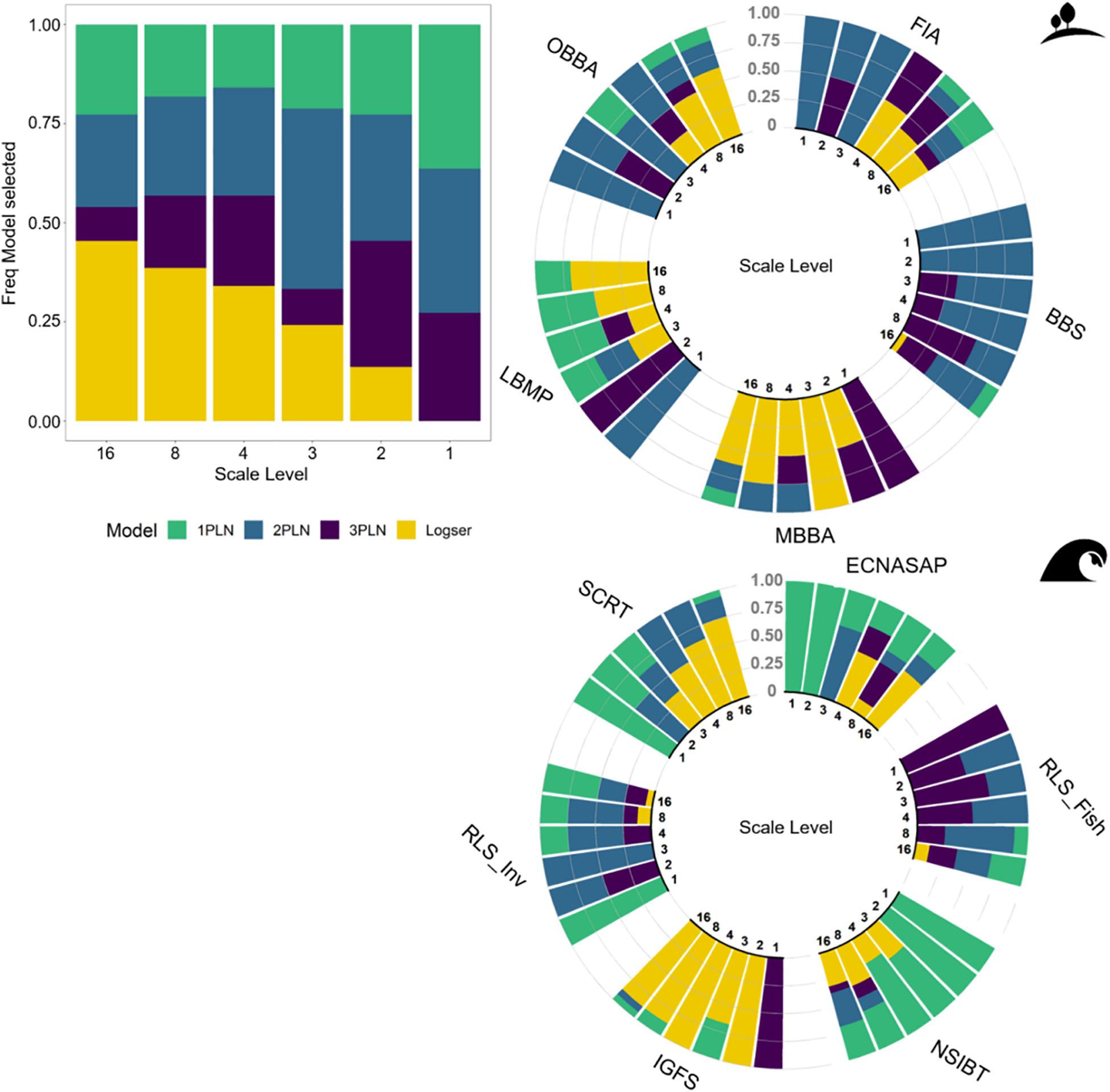
Figure 2. Effect of the sampling level on SAD shape across the scale gradient, showing the aggregated pattern across all the communities (barplot) and for each individual community in the circular plots for terrestrial (top) and marine (bottom) datasets. The colors represent the best model selected by AICc, i.e., either 1PLN, 2PLN, 3PLN, or logseries.
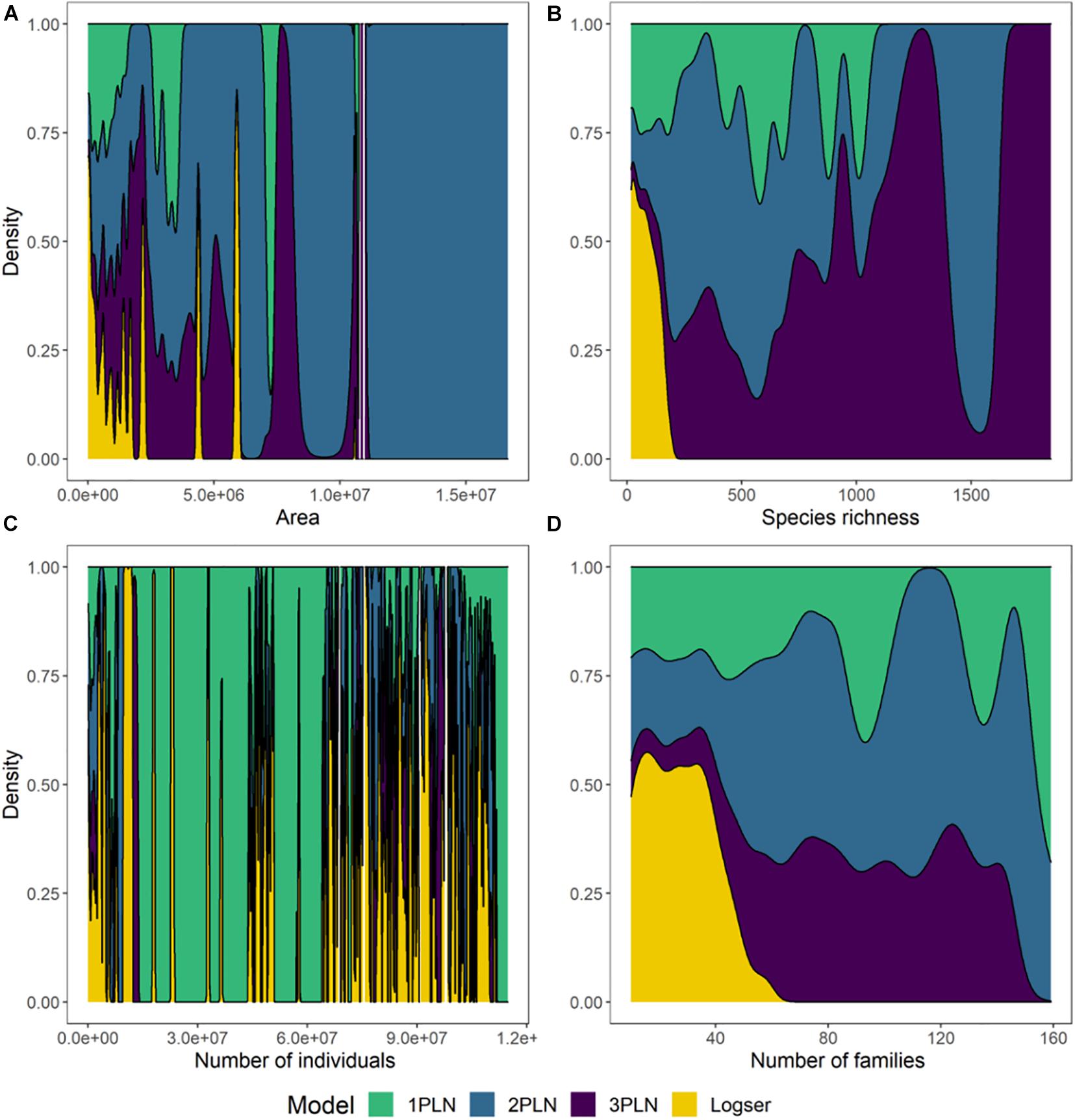
Figure 3. Effect of area sampled (A), species richness (B), total number of individuals (C), and number of families (D) on SAD shape (best model selected) aggregated across all the communities (see Supplementary Figure 1 for plots for each individual community). Plots were built using the function geom_density from the ggplot package in R (Wickham, 2009), which computes smoothed versions of histograms for continuous variables.
For the SADs selected as multimodal at the total extent, multimodal models most often provided the best fit across the scale gradient. This was the case for the FIA tree inventory, the BBS and OBBA bird, and the RLS fish datasets (Figure 2 and Supplementary Figure 1). The average ΔAICc for multimodality vs. non-multimodality across the scale gradient was 5.53 for FIA, 11.01 for BBS, 6.39 for OBBA and 9.77 for RLS_Fish (calculated as (min AICc 2PLN/3PLN–min AICc 1PLN/logser) across all sections). Additionally, some datasets exhibited the expected pattern of progressing from multimodality to either 1PLN or logseries as sampled area decreased (MBBA and LBMP birds and IGFS fish datasets; Figure 2 and Supplementary Figure 1). The datasets that were better fit by 1PLN at the total extent showed some variability in the best fit models as area decreased. For these, 1PLN was still frequently selected as best model, but both logseries and multimodal models were selected for smaller scales (ECNASAP and NSIBT fish, SCRT benthos and RLS invertebrate datasets; Figure 2 and Supplementary Figure 1).
Deviations between the empirical SADs and each model’s predictions support the results above. For the datasets with consistent support for multimodality across the scale gradient, logseries consistently and severely overestimated the number of singletons and rare species (i.e., octaves 1–2) across the scale gradient, while 1PLN often underestimated them. In addition, both logseries and 1PLN either over- or underestimated the number of species with intermediate to high abundances (Supplementary Figure 2). On average, for these assemblages, deviations were smaller for 2 or 3PLN at every scale (FIA, BBS, OBBA, and RLS_Fish; Supplementary Figure 2). For the remaining multimodal SADs at the total extent, logseries again overestimated the number of rare species, while the PLN mixtures exhibited large deviations between the observed number of species and the models’ predictions across the distribution and across the scale gradient (Supplementary Figure 2). For the datasets better fit by 1PLN at the total extent, for RLS invertebrates, deviations are much smaller on average for 2PLN at every scale, while both logseries and 1PLN underestimated the number of rare species. For the remaining SADs, there was no clear pattern, but logseries was systematically unable to accurately predict the rarest and intermediate abundance classes (Supplementary Figure 2).
Discussion
Our systematic assessment of empirical SADs shape across a wide scale gradient and taxa showed consistent variation in SAD shape. Furthermore, our results support previous findings of higher prevalence of multimodal SADs for larger areas or more taxonomically diverse communities (Antão et al., 2017), while the logseries never provided an adequate fit for larger and more diverse communities. In addition, we revealed a clear effect of area and taxonomic diversity in determining SAD shape, and a non-directional pattern for total abundance (for the aggregate communities’ results). Our findings clearly depart from two important macroecological theories predictions for the SAD. We discuss the implications of our results in turn below.
Variability in SAD Shape Across Spatial Scales
We compared the performance of different models to describe the SAD across a wide scale gradient to assess how the relative abundance patterns depend on spatial scale and also on taxonomic diversity (measured as species and family richness). For the communities selected as multimodal at the total extent, multimodality was consistently and strongly selected across the scale gradient, even for intense sampling effects of area and diversity. This indicates that multimodality is a robust feature of SADs and is indeed reflecting the structure of the underlying communities, rather than being a sampling (c.f. Barabás et al., 2013) or scaling artifact. The sections created across the scale gradient for these spatially large and taxonomically diverse datasets (FIA tree inventory, BBS and OBBA bird, and RLS fish surveys) still represent very large spatial extents. Additionally, due to the way the scale gradient was implemented, the spatial relationship between the sections is maintained. This further suggests that multimodality reflects the structure of the communities at these smaller scales, despite the marked decrease in number of species and total abundance as area sampled decreased. While using only AICc to select the best-fit model could potentially lead to the prevalence of multimodality being overestimated (Antão et al., 2017), there was consistent and strong support for 2PLN or 3PLN mixtures for these communities. Hence, we are confident the detection of multimodality in our analysis is robust. For these communities, SAD shape was overall conserved across a wide range of areas sampled, highlighting that dramatic shifts in key aspects of community structure are required for the overall SAD shape to change (e.g., Supp and Ernest, 2014). We further note that while we evaluated SAD scaling patterns using a single initial point to establish the scale gradient, in a related analysis we obtained consistent beta diversity scaling patterns across ten random initial points (Antão et al., 2019); we are thus confident the initial random point is unlikely to drive our results.
Clear shifts in SAD shape can provide information about relevant ecological and spatial factors affecting community structure at different scales. For the lognormal SADs at the total extent, but for which multimodality was frequently selected for smaller sections, this might be due to haphazard spatial decomposition of the community when splitting the total extent, and/or because of sampling effects. This can occur for instance if the communities become dominated by both rare and very abundant species, thus yielding multiple modes across the SAD (Gray et al., 2005; Green and Plotkin, 2007; see also Šizling et al., 2009b). When the common species are very abundant, 2PLN or 3PLN models are better able to accommodate both the rare and the most abundant species in the distribution, hence being selected despite the increase in number of parameters. Species spatial aggregation patterns can lead to one or a few species becoming extremely (proportionally) abundant for smaller areas. Simultaneously there is also a higher proportion of rare species in smaller samples, and hence a multimodal model provides a better fit than 1PLN. In contrast, logseries systematically failed to simultaneously accommodate rare and very abundant species.
Differences in species aggregation rates have been suggested to be related to the existence of multiple modes in both theoretical and empirical SADs (Green and Plotkin, 2007; Alonso et al., 2008; Dornelas and Connolly, 2008). Our findings suggest that multimodality occurring at smaller scales might be due to the spatial aggregation of individuals and species, where “hitting or missing” areas where a species is abundant can lead to the appearance of different modes. Hence, a multimodal model provides a better description for the SAD by accommodating both the rarest and the more abundant species, which neither the logseries nor a single PLN are able to do. Conspecific aggregation is one of the fundamental features of ecological communities (McGill, 2010). Our results suggest that species spatial aggregation is likely an important driver across scales [from local (see e.g., Šizling et al., 2009b) to truly continental scales] and taxa, which is consistent with a related analysis focusing on the scaling patterns of beta diversity (Antão et al., 2019). Finally, we also found transitions from logseries to lognormal as scale increased (Preston, 1948; Magurran, 2004). This finding is consistent with studies showing that the rate at which these transitions occur depend on species traits linked to the spatial distribution of individuals (Borda-de-Água et al., 2017; Dantas de Miranda et al., 2019). Overall, we have extended the range of scales usually evaluated in this type of analyses, both highlighting the importance of multimodal SADs, and showing clear patterns of SAD shape variability emerging across scales.
Comparison With Macroecological Theories
Our results clearly contrast with two key macroecological theories. The logseries was never selected as best fit for larger scales (i.e., larger areas, higher diversity or higher number of individuals) and was unable to accurately predict the abundances of both rare and common species. This clearly deviates from neutral models predictions of the logseries as the expected SAD for larger scales, including models with realistic speciation modes, that can produce more flexible metacommunity SADs and reduce the predicted number of singletons (Rosindell et al., 2010, 2011), but are still unable to provide adequate fit for large scale SADs (Fukaya et al., 2020) or accommodate multimodal SADs. Consistent with our results, a study of global rarity patterns in plants also found logseries distributions to inadequately fit global aggregate SAD, being outperformed by lognormal distributions (Enquist et al., 2019); interestingly multimodality was not evaluated. In addition, our findings also show a marked contrast with several studies reporting the success of METE models in characterizing general SAD shape (Harte et al., 2008; White et al., 2012; Xiao et al., 2015). For instance, the logseries was shown to provide a better fit to several empirical SADs with a wide range of “anchor scales” (White et al., 2012). This study included two communities analyzed here, namely the FIA tree and BBS bird datasets, for which multimodality was strongly selected along the scale gradient (although we did not analyze the smallest sample grain level). Yet, in agreement with our results, White et al. (2012) also reported that the logseries tended to overestimate richness for the lowest abundance classes, and the authors suggested that other METE formulations or neutral models could be used as alternatives, since they predict fewer singletons. While we have not directly analyzed either METE or neutral models, our results clearly illustrate that the logseries is not able to simultaneously deal with the rare and the abundant species tails. Hence, given that the logseries has been systematically outperformed, particularly for larger scales [here and in Antão et al. (2017) and Enquist et al. (2019)], it is unlikely that the logseries is an adequate descriptor of SADs across spatial scales. The same inability has been shown for the lognormal distribution, explicitly linked to species turnover and spatial aggregation patterns between the smaller scale SADs being pooled together in the theorethical famework proposed by Šizling et al. (2009a, b). A critical development is then to accommodate the variability in SAD shape with spatial scale, and crucially to include multimodality, given its high prevalence across all scales.
Our results do not invalidate the logseries or the lognormal as “realistic functional forms” for the SAD, as both were selected as best model for several communities (here, as well as in Antão et al., 2017). What our results clearly show is that the logseries is neither adequate as the single SAD distribution, as METE suggests, nor is it more likely to describe SADs at larger scales, contrary to NTB predictions (Hubbell, 2001; Pueyo et al., 2007; Rosindell et al., 2010). A model extending the neutral theory by incorporating size variation and growth dynamics [the size-structured neutral theory model (SSNT)] still assumes a logseries SAD (O’Dwyer et al., 2009). Comparisons of different model formulations for both METE and SSNT showed a better performance for the latter (O’Dwyer et al., 2009; Xiao et al., 2016), with the authors arguing that METE’s constraints are not fully capturing relevant biological processes influencing community structure. Furthermore, because derivations for other macroecological patterns depend on a logseries SAD (Harte et al., 2008), testing other SAD distributions to ensure those derivations are robust is warranted. For instance, Šizling et al. (2011) showed that incorporating spatial turnover at different scales affected local species area relationships derived from METE. Moreover, neither neutral nor METE models account for multiple modes in SADs, not to their higher prevalence at larger scales and for more diverse communities. Our results also suggest that the combination of S and N is not sufficient to determine SAD shape across spatial scales (White et al., 2012; Locey and White, 2013; Xiao et al., 2015), specifically as the total abundance across the scale gradient did not exhibit any systematic effect on SAD shape (for the aggregated results). Nonetheless, both area and species richness showed a strong influence on SAD shape, although the two variables are also strongly correlated (Rosenzweig, 1995). One of the advantages of using the METE approach is being able to interpret deviations from the expected distributions solely constrained by richness and abundance as evidence that other ecological features must be important in structuring communities (Harte et al., 2008; White et al., 2012; Xiao et al., 2016). Here, we show this must be the case for several large-scale empirical communties, and suggest that spatial aggregation patterns and ecological heterogeneity as potential such factors.
One potential explanation for the departure of the findings presented here from the two macroecological frameworks considered could be the scale gradient examined. This gradient spanned several orders of magnitude, and included very large areas, even for the smallest levels analyzed. Hence, it is possible that discrepancies between our results and those theoretical predictions might be at least partially attributable to differences in the spatial scales investigated (as noted above for the FIA and BBS datasets). The same is true for the spatial theory developed by Šizling et al. (2009a, b), which mainly focused on upscaling SADs for larger plots, but which remain much smaller than the smallest level in our analysis. In addition, and while we analyzed extensively and consistently sampled datasets with hundreds to several thousands of samples, it is particularly hard to obtain thorough abundance records at such large extents. Thus, sampling effects could also potentially influence our results, particularly at the largest scales, where sampling effects known to affect SAD shape may be more severe. Nonetheless, our results strongly support the suggestion that both NTB and METE might be more adequate for smaller scales (smaller areas and/or fewer individuals) (McGill, 2010), while the traditional SAD distributions are unable to accommodate SAD shape variability with scale, as we have clearly shown with consistent empirical patterns across taxa, and for both marine and terrestrial habitats.
Conclusion
Spatial scale and taxonomic diversity emerged as major drivers of variability in SAD shape. The systematic assessment of SADs at different spatial scales and for different taxa allows us to make stronger inferences about the commonness and rarity of species across scales. Our findings clearly show that neither NTB nor METE formulations are able to accommodate the variability in SADs shape across spatial scales. The interplay of SAD shape at different scales can highlight important mechanisms acting on ecological communities, namely both inter- and intraspecific spatial patterns that lead to different SAD shape as spatial scale changes. Furthermore, a critical development for macroecological theories is to predict or accommodate multimodal SADs, and crucially to incorporate the effect of spatial scale and ecological heterogeneity in determining SAD shape.
Data Availability Statement
Publicly available datasets were analyzed in this study. This data can be found here: All the datasets used in this study can be accessed through either the BioTIME database (on Zenodo—https://doi.org/10.5281/zenodo.1211105; or the BioTIME website—http://biotime.st-andrews.ac.uk/) or the EcoData Retriever, or alternatively from the original sources cited.
Author Contributions
LA and MD designed the study. LA assembled the data, performed all the analyses, and wrote the first draft of the manuscript. All authors have discussed the results and contributed extensively to the final manuscript.
Funding
LA was supported by the Fundação para a Ciência e Tecnologia, Portugal (POPH/FSE SFRH/BD/90469/2012) and by the Jane and Aatos Erkko Foundation. AM and the BioTIME database were funded by the European Research Council grants AdG BioTIME (250189) and PoC BioCHANGE (727440). MD was funded by a Leverhulme Fellowship and by the John Templeton Foundation (grant #60501 “Putting the Extended Evolutionary Synthesis to the Test”). Open access was funded by Helsinki University Library.
Conflict of Interest
The authors declare that the research was conducted in the absence of any commercial or financial relationships that could be construed as a potential conflict of interest.
Acknowledgments
We are grateful to all the scientists, data collectors and their funders for making data publicly available. We thank the University of St. Andrews Bioinformatics Unit (Wellcome Trust ISSF grant [105621/Z/14/Z]). Faye Moyes assisted with data management. The two icons in Figure 2 are from the Noun Project under CCBY license: land by A. Skowalsky, and wave by B. Farias.
Supplementary Material
The Supplementary Material for this article can be found online at: https://www.frontiersin.org/articles/10.3389/fevo.2021.626730/full#supplementary-material
Footnotes
References
Alonso, D., Ostling, A., and Etienne, R. S. (2008). The implicit assumption of symmetry and the species abundance distribution. Ecol. Lett. 11, 93–105. doi: 10.1111/j.1461-0248.2007.01127.x
Antão, L. H., Connolly, S. R., Magurran, A. E., Soares, A., and Dornelas, M. (2017). Prevalence of multimodal species abundance distributions is linked to spatial and taxonomic breadth. Glob. Ecol. Biogeogr. 26, 203–215. doi: 10.1111/geb.12532
Antão, L. H., McGill, B., Magurran, A. E., Soares, A. M. V. M., and Dornelas, M. (2019). β-diversity scaling patterns are consistent across metrics and taxa. Ecography 42, 1012–1023. doi: 10.1111/ecog.04117
Barabás, G., D’Andrea, R., Rael, R., Meszéna, G., and Ostling, A. (2013). Emergent neutrality or hidden niches? Oikos 122, 1565–1572. doi: 10.1111/j.1600-0706.2013.00298.x
Bivand, R., and Rundel, C. (2016). rgeos: Interface to Geometry Engine - Open Source (GEOS). R package version 0.3-19.
Borda-de-Água, L., Borges, P. A. V., Hubbell, S. P., and Pereira, H. M. (2012). Spatial scaling of species abundance distributions. Ecography 35, 549–556. doi: 10.1111/j.1600-0587.2011.07128.x
Borda-de-Água, L., Hubbell, S. P., and McAllister, M. (2002). Species-area curves, diversity indices, and species abundance distributions: a multifractal analysis. Am. Nat. 159, 138–155. doi: 10.1086/324787
Borda-de-Água, L., Whittaker, R. J., Cardoso, P., Rigal, F., Santos, A. M. C., Amorim, I. R., et al. (2017). Dispersal ability determines the scaling properties of species abundance distributions: a case study using arthropods from the Azores. Sci. Rep. 7:3899. doi: 10.1038/s41598-017-04126-5
Brown, S. K. R., Zwanenburg, K., and Branton, R. (2005). East Coast North America Strategic Assessment Groundfish Atlas - ECNASAP. OBIS Canada. Dartmouth, NS: Bedford Institute of Oceanography. Available online at: http://www.iobis.org/ (accessed on 2013).
Bulmer, M. (1974). On fitting the Poisson lognormal distribution to species-abundance data. Biometrics 30, 101–110. doi: 10.2307/2529621
Burnham, K. P., and Anderson, D. R. (2002). Model Selection and Multimodel Inference: A Practical Information-Theoretic Approach, 2nd Edn. New York, NY: Springer.
Condit, R. S., Ashton, P. S., Baker, P. J., Bunyavejchewin, S., Gunatilleke, S., Gunatilleke, N., et al. (2000). Spatial patterns in the distribution of tropical tree species. Science 288, 1414–1418. doi: 10.1126/science.288.5470.1414
Connolly, S. R., Hughes, T. P., Bellwood, D. R., and Karlson, R. H. (2005). Community structure of corals and reef fishes at multiple scales. Science 309, 1363–1365. doi: 10.1126/science.1113281
Dantas de Miranda, M., Borda-de-Água, L., Pereira, H. M., and Merckx, T. (2019). Species traits shape the relationship between local and regional species abundance distributions. Ecosphere 10:e02750. doi: 10.1002/ecs2.2750
DATRAS (2010a). Fish trawl survey: ICES North Sea International Bottom Trawl Survey for commercial fish species. ICES Database of trawl surveys (DATRAS). Copenhagen: International Council for the Exploration of the Sea (ICES). Available online at: http://www.emodnet-biology.eu/data-catalog??module=dataset&dasid=2763 (accessed on 2013).
DATRAS (2010b). Fish trawl survey: Irish Ground Fish Survey for commercial fish species. ICES Database of trawl surveys (DATRAS). Copenhagen: International Council for the Exploration of the Sea (ICES). Available online at: www.emodnet-biology.eu/data-catalog?module=dataset&dasid=2762 (accessed on 2013).
Dewdney, A. K. (1998). A general theory of the sampling process with applications to the “veil line.”. Theor. Popul. Biol. 54, 294–302. doi: 10.1006/tpbi.1997.1370
Dornelas, M., Antão, L. H., Moyes, F., Bates, A. E., Magurran, A. E., Adam, D., et al. (2018). BioTIME: a database of biodiversity time series for the anthropocene. Glob. Ecol. Biogeogr. 27, 760–786. doi: 10.1111/geb.12729
Dornelas, M., and Connolly, S. R. (2008). Multiple modes in a coral species abundance distribution. Ecol. Lett. 11, 1008–1016. doi: 10.1111/j.1461-0248.2008.01208.x
Dornelas, M., Connolly, S. R., and Hughes, T. P. (2006). Coral reef diversity refutes the neutral theory of biodiversity. Nature 440, 80–82. doi: 10.1038/nature04534
Edgar, G. J., and Stuart-Smith, R. D. (2008). Reef Life Survey (RLS): Invertebrates. Battery Point, TAS: Institute for Marine and Antarctic Studies (IMAS). Available online at: https://catalogue-rls.imas.utas.edu.au/geonetwork/srv/en/metadata.show?uuid=60978150-1641-11dd-a326-00188b4c0af8b (accessed on 2016).
Edgar, G. J., and Stuart-Smith, R. D. (2014a). Reef Life Survey (RLS): Global reef fish dataset. Battery Point, TAS: Institute for Marine and Antarctic Studies (IMAS). Available online at: https://catalogue-rls.imas.utas.edu.au/geonetwork/srv/en/metadata.show?uuid=9c766140-9e72-4bfb-8f04-d51038355c59 (accessed on 2016).
Edgar, G. J., and Stuart-Smith, R. D. (2014b). Systematic global assessment of reef fish communities by the Reef Life Survey program. Sci. Data 1:140007. doi: 10.1038/sdata.2014.7
Enquist, B. J., Feng, X., Boyle, B., Maitner, B., Newman, E. A., Jørgensen, P. M., et al. (2019). The commonness of rarity: global and future distribution of rarity across land plants. Sci. Adv. 5:eaaz0414. doi: 10.1126/sciadv.aaz0414
Etienne, R. S. (2005). A new sampling formula for neutral biodiversity. Ecol. Lett. 8, 253–260. doi: 10.1111/j.1461-0248.2004.00717.x
Etienne, R. S. (2007). A neutral sampling formula for multiple samples and an “exact” test of neutrality. Ecol. Lett. 10, 608–618. doi: 10.1111/j.1461-0248.2007.01052.x
Etienne, R. S. (2009). Maximum likelihood estimation of neutral model parameters for multiple samples with different degrees of dispersal limitation. J. Theor. Biol. 257, 510–514. doi: 10.1016/j.jtbi.2008.12.016
Fisher, R., Corbet, A., and Williams, C. (1943). The relation between the number of species and the number of individuals in a random sample of an animal population. J. Anim. Ecol. 12, 42–58. doi: 10.2307/1411
Fukaya, K., Kusumoto, B., Shiono, T., Fujinuma, J., and Kubota, Y. (2020). Integrating multiple sources of ecological data to unveil macroscale species abundance. Nat. Commun. 11:1695. doi: 10.1038/s41467-020-15407-5
Gray, J. S., Bjørgesæter, A., and Ugland, K. I. (2005). The impact of rare species on natural assemblages. J. Anim. Ecol. 74, 1131–1139. doi: 10.1111/j.1365-2656.2005.01011.x
Gray, J. S., Bjørgesæter, A., and Ugland, K. I. (2006). On plotting species abundance distributions. J. Anim. Ecol. 75, 752–756. doi: 10.1111/j.1365-2656.2006.01095.x
Green, J. L., and Plotkin, J. B. (2007). A statistical theory for sampling species abundances. Ecol. Lett. 10, 1037–1045. doi: 10.1111/j.1461-0248.2007.01101.x
Harte, J., and Newman, E. A. (2014). Maximum information entropy: a foundation for ecological theory. Trends Ecol. Evol. 29, 384–389. doi: 10.1016/j.tree.2014.04.009
Harte, J., Zillio, T., Conlisk, E., and Smith, A. (2008). Maximum entropy and the state-variable approach to macroecology. Ecology 89, 2700–2711. doi: 10.1890/07-1369.1
Hubbell, S. P. (2001). The Unified Neutral Theory of Biodiversity and Biogeography. Princeton, NY: Princeton University Press.
Levin, S. (1992). The problem of pattern and scale in ecology: the Robert H. MacArthur award lecture. Ecology 73, 1943–1967. doi: 10.2307/1941447
Locey, K. J., and White, E. P. (2013). How species richness and total abundance constrain the distribution of abundance. Ecol. Lett. 16, 1177–1185. doi: 10.1111/ele.12154
Magurran, A. E., and Henderson, P. A. (2003). Explaining the excess of rare species in natural species abundance distributions. Nature 422, 714–716. doi: 10.1038/nature01547
May, R. M. (1975). “Patterns of species abundance and diversity” in Ecology and Evolution of Communities, eds M. L. Cody and J. M. Diamond (Cambridge, MA: Belknap Press of Harvard University Press), 81–120.
McGill, B. J. (2003a). A test of the unified neutral theory of biodiversity. Nature 422, 881–885. doi: 10.1038/nature01569.1
McGill, B. J. (2003b). Does Mother Nature really prefer rare species or are log-left-skewed SADs a sampling artefact? Ecol. Lett. 6, 766–773. doi: 10.1046/j.1461-0248.2003.00491.x
McGill, B. J. (2010). Towards a unification of unified theories of biodiversity. Ecol. Lett. 13, 627–642. doi: 10.1111/j.1461-0248.2010.01449.x
McGill, B. J., Etienne, R. S., Gray, J. S., Alonso, D., Anderson, M. J., Benecha, H. K., et al. (2007). Species abundance distributions: moving beyond single prediction theories to integration within an ecological framework. Ecol. Lett. 10, 995–1015. doi: 10.1111/j.1461-0248.2007.01094.x
McGlinn, D., and White, E. (2015). ecoretriever: R Interface to the EcoData Retriever. R package version 0.2.1. Available online at: https://cran.r-project.org/package=ecoretriever (accessed on 2016).
Morris, B. D., and White, E. P. (2013). The ecodata retriever: improving access to existing ecological data. PLoS One 8:e65848. doi: 10.1371/journal.pone.0065848
NatureCounts (2012a). Maritimes Breeding Bird Atlas (2006-2010): point count data. NatureCounts, a node Avian Knowledge Network. Bird Studies, Canada. Available online at: http://www.birdscanada.org/birdmon/ (accessed on 2012).
NatureCounts (2012b). Ontario Breeding Bird Atlas (2001-2005): Point Count Data. NatureCounts, a Node Avian Knowledge Network. Bird Studies, Canada. Available online at: http://www.birdscanada.org/birdmon/ (accessed on 2012).
O’Dwyer, J. P., Lake, J. K., Ostling, A., Savage, V. M., and Green, J. L. (2009). An integrative framework for stochastic, size-structured community assembly. Proc. Natl. Acad. Sci. U.S.A. 106, 6170–6175. doi: 10.1073/pnas.0813041106
Pardieck, K. L., Ziolkowski, D. J. J., Hudson, M.-A. R., and Campbell, K. (2016). North American Breeding Bird Survey Dataset 1966 - 2015, Version 2015.1. Laurel, MD: U.S. Geological Survey, Patuxent Wildlife Research Center, doi: 10.5066/F7C53HZN
Preston, F. (1948). The commonness, and rarity, of species. Ecology 29, 254–283. doi: 10.2307/1930989
Pueyo, S., He, F., and Zillio, T. (2007). The maximum entropy formalism and the idiosyncratic theory of biodiversity. Ecol. Lett. 10, 1017–1028. doi: 10.1111/j.1461-0248.2007.01096.x
R Core Team (2017). R: A Language and Environment for Statistical Computing. Vienna: R Foundation for Statistical Computing.
Rosenzweig, M. L. (1995). Species Diversity in Space and Time. Cambridge: Cambridge University Press.
Rosindell, J., and Cornell, S. J. (2013). Universal scaling of species-abundance distributions across multiple scales. Oikos 122, 1101–1111. doi: 10.1111/j.1600-0706.2012.20751.x
Rosindell, J., Cornell, S. J., Hubbell, S. P., and Etienne, R. S. (2010). Protracted speciation revitalizes the neutral theory of biodiversity. Ecol. Lett. 13, 716–727. doi: 10.1111/j.1461-0248.2010.01463.x
Rosindell, J., Hubbell, S. P., and Etienne, R. S. (2011). The unified neutral theory of biodiversity and biogeography at age ten. Trends Ecol. Evol. 26, 340–348. doi: 10.1016/j.tree.2011.03.024
Šizling, A. L., Kunin, W. E., Sizlingová, E., Reif, J., and Storch, D. (2011). Between geometry and biology: the problem of universality of the species-area relationship. Am. Nat. 178, 602–611. doi: 10.1086/662176
Šizling, A. L., Storch, D., Reif, J., and Gaston, K. J. (2009a). Invariance in species-abundance distributions. Theor. Ecol. 2, 89–103. doi: 10.1007/s12080-008-0031-3
Šizling, A. L., Storch, D., Sizlingova, E., Reif, J., and Gaston, K. J. (2009b). Species abundance distribution results from a spatial analogy of central limit theorem. Proc. Natl. Acad. Sci. U.S.A. 106, 6691–6695. doi: 10.1073/pnas.0810096106
Supp, S. R., and Ernest, S. K. M. (2014). Species-level and community-level responses to disturbance: a cross-community analysis. Ecology 95, 1717–1723. doi: 10.1890/13-2250.1
USDA Forest Service (2010). Forest Inventory and Analysis National Core Field Guide (Phase 2 and 3). Version 4.0. Washington, D.C: USDA Forest Service, Forest Inventory and Analysis.
USFS (2012). Landbird Monitoring Program (UMT-LBMP). US Forest Service. Available online at: http://www.avianknowledge.net/ (accessed on 2012).
Volkov, I., Banavar, J. R., Hubbell, S. P., and Maritan, A. (2003). Neutral theory and relative species abundance in ecology. Nature 424, 1035–1037. doi: 10.1038/nature01883
Volkov, I., Banavar, J. R., Hubbell, S. P., and Maritan, A. (2007). Patterns of relative species abundance in rainforests and coral reefs. Nature 450, 45–49. doi: 10.1038/nature06197
Wade, E. J. (2011). Snow Crab Research Trawl Survey Database (Southern Gulf of St. Lawrence, Gulf region, Canada) From 1988 to 2010. Dartmouth, NS: Bedford Institute of Oceanography Available online at: http://iobis.org/ (accessed on 2012).
White, E. P., Thibault, K. M., and Xiao, X. (2012). Characterizing species abundance distributions across taxa and ecosystems using a simple maximum entropy model. Ecology 93, 1772–1778. doi: 10.1890/11-2177.1
Wickham, H. (2009). ggplot2: Elegant Graphics for Data Analysis. New York: Springer-Verlag New York.
Woudenberg, S. W., Conkling, B. L., O’Connell, B. M., LaPoint, E. B., Turner, J. A., and Waddell, K. L. (2010). The Forest Inventory and Analysis Database: Database description and users manual version 4.0 for Phase 2. General Technical Report No. RMRSGTR-245. Fort Collins, CO: Department of Agriculture, Forest Service, Rocky Mountain Research Station.
Xiao, X., McGlinn, D. J., and White, E. P. (2015). A strong test of the maximum entropy theory of ecology. Am. Nat. 185, E70–E80. doi: 10.1086/679576
Xiao, X., O’Dwyer, J. P., and White, E. P. (2016). Comparing process-based and constraint-based approaches for modeling macroecological patterns. Ecology 97, 1228–1238. doi: 10.1890/15-0962.1
Keywords: spatial scale, biodiversity, community structure, multimodality, macroecology, maximum entropy theory of ecology, neutral theory of biodiversity and biogeography
Citation: Antão LH, Magurran AE and Dornelas M (2021) The Shape of Species Abundance Distributions Across Spatial Scales. Front. Ecol. Evol. 9:626730. doi: 10.3389/fevo.2021.626730
Received: 06 November 2020; Accepted: 08 March 2021;
Published: 07 April 2021.
Edited by:
Luís Borda-de-Água, Universidade do Porto, PortugalReviewed by:
Tom Matthews, University of Birmingham, United KingdomDavid Storch, Charles University, Czechia
Copyright © 2021 Antão, Magurran and Dornelas. This is an open-access article distributed under the terms of the Creative Commons Attribution License (CC BY). The use, distribution or reproduction in other forums is permitted, provided the original author(s) and the copyright owner(s) are credited and that the original publication in this journal is cited, in accordance with accepted academic practice. No use, distribution or reproduction is permitted which does not comply with these terms.
*Correspondence: Laura H. Antão, laura.antao@helsinki.fi
†ORCID: Laura H. Antão, orcid.org/0000-0001-6612-9366; Anne E. Magurran, orcid.org/0000-0002-0036-2795; Maria Dornelas, orcid.org/0000-0003-2077-7055