A Test for the Underlying State-Structure of Hidden Markov Models: Partially Observed Capture-Recapture Data

Hidden Markov models (HMMs) are being widely used in the field of ecological modeling, however determining the number of underlying states in an HMM remains a challenge. Here we examine a special case of capture-recapture models for open populations, where some animals are observed but it is not possible to ascertain their state (partial observations), whilst the other animals' states are assigned without error (complete observations). We propose a mixture test of the underlying state structure generating the partial observations, which assesses whether they are compatible with the set of states observed in the complete observations. We demonstrate the good performance of the test using simulation and through application to a data set of Canada Geese.

1. Introduction

Besides its known use for the estimation of the size of a closed population (Pledger, 2000; Yang and Chao, 2005; Bartolucci and Pennoni, 2007) originating in the work of Otis et al. (1978), capture-recapture is also a widely used technique to follow the dynamics of open animal populations (Cormack, 1964; Williams et al., 2002). The protocol remains the same: animals are uniquely marked, then released and resighted/recaptured at subsequent sampling occasions. In the multi-state framework (Lebreton et al., 2009), at each occasion, individual animals' states are recorded upon resighting; if an animal is not seen at a given occasion, this is denoted by a 0. If it is seen, a code, commonly a number, specifies the state (see example data set in Supplementary Material). Hence, the data resulting from a multi-state capture-recapture experiment consists of individual encounter histories, formed by the series of records made for each animal. Multi-state models allow the estimation of the survival and transition probabilities of animals between the states, whilst accounting for imperfect detection. Within this modeling framework, states are assumed to be assigned without error (Kendall, 2004). However, this assumption can be unrealistic in certain situations such as the assessment of sex in a monomorphic species or of health status when biological testing is not possible in the field. Pradel (2005) developed multievent models to account for the uncertainty in state assignment. These models belong to the family of Hidden Markov Models (Zucchini et al., 2016) and distinguish the events, which are observed, from the states, which are underlying. The process governing the transitions between states is Markovian (generally assumed of order 1) and the events are generated by the states. Multievent models have a structural absorbing state (death). Transitions are almost systematically time-dependent, which precludes the consideration that the system has reached an equilibrium. Also, because the chance that an individual is missed is state dependent, non-observations cannot be considered as data missing at random. They are informative events like any other outcome of the experiment.

In this paper we focus on a special case of multievent models, where, at a given occasion, the state cannot be ascertained for a proportion of the observed animals, leading to partial observations, whilst the underlying states are directly observable for the other observed animals (complete observations). In analysing this type of data, it is usually assumed that the range of potential states is limited to the set of states observed in the complete observations (see Figure 1). However, some states may not be directly observable, yet capable of generating partial observations (see Figure 2). We propose a new diagnostic tool to assess whether the partial observations are consistent with being generated only by the directly observable states (H₀) or whether partial observations may be generated by at least one additional unidentified state never directly observed (H₁). For instance, in a study of movements, animals may move between the set of monitored sites, where observations are made, and an additional unmonitored site (see scenarios 2PO and 3PO of the Canada geese example below). Such a test is currently lacking in the literature and pragmatic approaches need to be taken (see for example Pohle et al., 2017).

FIGURE 1

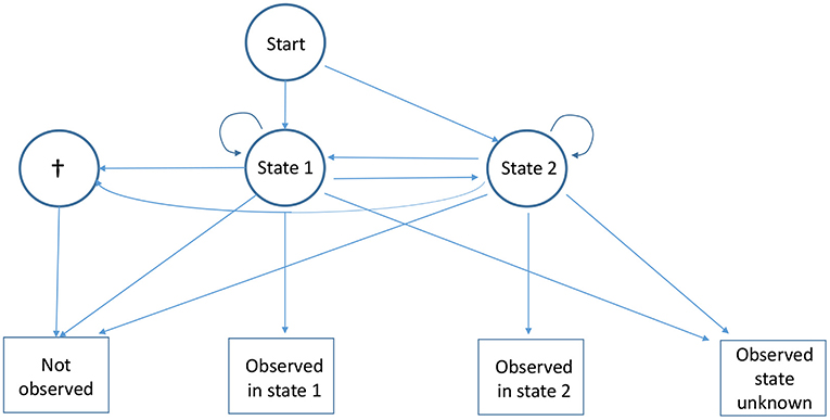
Figure 1. Diagram of the capture recapture multievent model for partial observations with two observable live states under the null hypothesis. The state “dead” is represented by †. Four events are generated by the three states: “Not observed,” which is obligatory for the state “dead”; two complete observations, “Observed in state 1” and “Observed in state 2”; and the partial observation “Observed state unknown,” which may be generated by either live state.

FIGURE 2

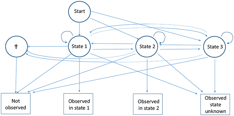
Figure 2. Diagram of the capture recapture multievent model for partial observations with two observable live states under the alternative hypothesis where there is one additional non-observable live state (state 3). This last state is never recognized upon observation. See Figure 1 for more details.

Our test builds on the approach used by Pradel et al. (2003) to construct a mixture test for the multi-state framework, as well as the sufficient statistics and likelihood components developed by King and McCrea (2014) for the special case of partial observations. Indeed, we show that if partial observations are generated only by the directly observable states, the number of animals partially observed at a given occasion i and re-observed later in a known state, follows a conditional multinomial distribution, which is a mixture of the conditional multinomial distributions followed by the number of animals released at occasion i in the observable states. Based on this mixture property, we then use usual goodness-of-fit measures to assess the fit of a model where only the directly observable states generate the partial observations.

We use simulation to empirically assess the test and apply it to a Canada Geese, Branta canadensis, dataset (Hestbeck et al., 1991), in which we artificially create partial observations. This demonstrates that the test can work well under practical settings and sample size.

2. Partially Observed Capture-Recapture Data and Mixture Properties

Consider a capture-recapture experiment with T sampling occasions and R live states. If individuals are assigned to state r upon capture, this is done with certainty and the corresponding event is denoted by r: “observed in state r.” When an individual's state cannot be determined, the corresponding event, a partial observation, is denoted by U: “observed with state unknown” and the animal can be in any one of the underlying R states.

The state and time-dependent parameters of the partial observation capture-recapture model (King and McCrea, 2014) are defined by:

• ${\varphi }_t^r$ is the probability an individual in state r at time t survives until t + 1, for t = 1, …, T − 1 and r = 1, …, R.

• $p_t^r$ is the probability of recapture at time t for an individual in state r, for t = 2, …, T.

• ${\psi }_t^{r,s}$ is the probability an individual is in state s at time t + 1 given that it was in state r at time t and is alive at t + 1, for t = 1, …, T − 1, r = 1, …, R, and s = 1, …, R.

• ${\alpha }_t^r$ is the probability an individual is assigned to state r given it was recaptured at time t and in state r at that time, for t = 2, …, T and r = 1, …, R. ${\beta }_t^r=1-{\alpha }_t^r$ is then defined as the probability an individual is assigned as unknown (U) at time t given the individual is recaptured, and in state r at this time, for t = 2, …, T and r = 1, …, R. An animal is either assigned to the correct state or unassigned but there are no assignment error.

• ${\pi }_t^r$ is the initial state probability of individuals in an unknown state when first observed. This corresponds to the probability an individual is in state r at time t, given it was first observed in U at t, for t = 1, …, T − 1.

The sufficient statistics are based on partitioning the encounter histories (EH) into the following pieces: the EH between observations in two known states; the EH between first observation in unknown state and first re-observation in a known state; the EH following the last observation in a known state; and the EH following the first observation in an unknown state, for animals who are never seen in a known state (Table 1 provides examples). We define the following sufficient statistics:

• $n_{t_1,t_2+1}^{r,z_{(t_1+1):(t_2)},s}$ denotes the number of animals observed at time t₁ in known state r, next observed in known state s at t₂ + 1 with partial capture history z_{(t1 + 1):(t2)} between these two time points. Note that when t₁ = t₂, z_{(t1 + 1):(t2)} is denoted by −.

• $w_{t_1,t_2+1}^{U,z_{(t_1+1):(t_2)},s}$ denotes the number of animals observed for the first time at t₁ in an unknown state, re-observed for the first time in known state s at time t₂ + 1 with partial capture history z_{(t1 + 1):(t2)} between these two time points.

• $v_{t_1}^r$ is the number of animals observed in known state r at t₁ and never seen again in a known state (i.e., never seen again or only ever re-observed in an unknown state).

• $b_{t_1}^U$ is the number of animals first observed in an unknown state at t₁ and never seen again in a known state.

TABLE 1

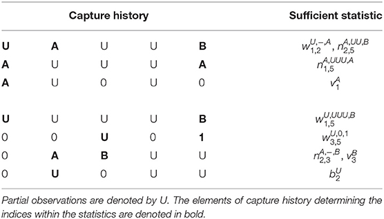
Table 1. Illustrating how example individual capture histories contribute to the sufficient statistic terms, for a capture-recapture experiment with two observable states A, B, and five sampling occasions.

Building upon the notation and probabilities introduced in the previous section, we will demonstrate that the number of animals partially observed at time i and later seen again in a known state, follows a multinomial distribution which is a mixture of the multinomial distributions of the animals released in a known state at time i and seen again in a known state later. The multinomial cells correspond to the time and state of the first re-observation in a known state after time i.

The mixture property is illustrated for a simple example in Table 2 for occasion i = 2 of a T = 4 occasion capture-recapture study with two live states A and B. The number of animals released in state A at occasion 1 first re-captured in a known state at the different occasions, and those never seen again in a known state, follow a multinomial distribution (row 1). Similarly for those released in state B at occasion 1 (row 2), and those first released in an unknown state at occasion 1 (row 3) and at occasion 2 (row 4).

TABLE 2

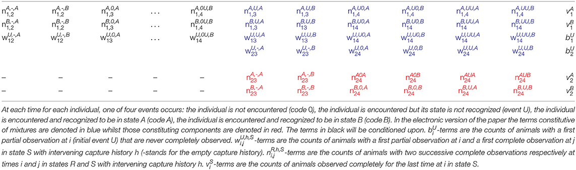
Table 2. The sufficient statistics for multinomial distributions corresponding to individuals released before or at i = 2 in an capture-recapture experiment with four occasions where individuals can be in any of two live states.

When the number of sampling occasions increases, capture histories are long and there are a great number of possible intermediate capture histories, formed of combinations of 0s and Us, before the first observation in a known state appears. In order to lower the chances of a sparse table, we opt to build the multinomials based on the time and state of the first known re-observed state, thus pooling over all possible intermediate capture histories.

In Supplementary Material (section 2), we show that the number of animals previously released in a known state r, partially observed at occasion i and re-observed later in a known state, follows a conditional multinomial distribution, which is a mixture of the conditional multinomial distributions followed by the animals released at occasion i in the observable states. We also show that the number of animals first released before i or at i in an unknown state, partially observed at occasion i and re-observed later in a known state, follows a conditional multinomial distribution (denoted in blue in Table 1), which is a mixture of the conditional multinomial distributions followed by the animals released at i in the observable states (denoted in red in Table 1).

Using the following property cited from Pradel et al. (2003): “if B1 and B2 are mutually independent stochastic vectors, which are multinomially distributed, and if M1 and M2 are mutually independent stochastic vectors whose distributions are separately mixtures of the distributions of B1 and B2, then the distribution of M1+M2 is itself a mixture of the distributions of B1 and B2,” the conditional multinomials of the animals released in a known state or first released in an unknown state before or at i, and partially observed at i can be pooled as shown in Table 3. Thus, the table used to test the mixture property of partial observations at occasion i is given in Table 3.

TABLE 3

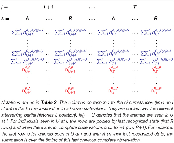
Table 3. Table used for testing the mixture property of partial observations at occasion i in a capture-recapture experiment with T occasions where individuals can be in any of R live states.

3. Testing the Underlying State Structure Generating the Partial Observations

Based on the mixture property of partial observations at a given occasion demonstrated in the previous section, we use the Multinomial Maximum Likelihood Mixture approach (MMLM) developed by Yantis et al. (1991) to assess the goodness-of-fit of a model where the partial observations are generated only by the directly observable states. The MMLM approach is targeted to mixtures of multinomial distributions and is used when independent samples are available from both the mixtures and their associated components. This approach consists of two steps: first estimating the cell probabilities of the mixture components and the mixing weights via maximum-likelihood, then assessing the goodness-of-fit of the hypothesized model structure (mixtures and associated components) using a classical measure of comparison between observed and expected frequencies.

Hence, based on the mixture property of the partial observations demonstrated in the Supplementary Material and reported in section 2, there is no need to estimate the numerous capture-recapture parameters for the purpose of the test, the information needed is summarized in simpler terms: one parameter per component-cell and the mixing weights as illustrated in Table 4.

TABLE 4

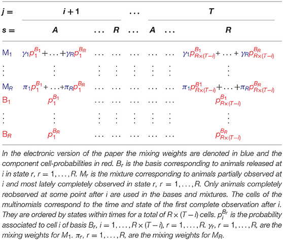
Table 4. Simple model structure of mixtures and associated components used to test the mixture property.

For the goodness-of-fit assessment, various statistics based on the distance between expected values under the model and observed values may be considered: Pearson's χ², the log-likelihood ratio statistic G² (Cressie and Read, 1988, p. 10); and more generally, due to the different properties of these statistics depending on the alternatives or sparseness of the table, the power-divergence family of statistics (Cressie and Read, 1988), which encompasses G² and χ² as special cases. Within this paper, we present the results obtained with Pearson's χ² as all the various statistics used gave similar results.

Under the null hypothesis, animals partially observed at i and re-observed later in a known state are consistent with being a mixture of animals observed in the directly observable states at i and re-observed in the same conditions: the partial observations are generated solely by the observable states (Figure 1). Using the usual H₀ notation for the null hypothesis and H₁ for the alternative, $H_1=\overline{H_0}$. A large array of situations come under the alternative hypothesis: from the partial observations being generated by the directly observable states and another state which is never directly observable (Figure 2) to the most extreme case of partial observations all being generated only by one (or more) states which are never directly observable.

Under the null hypothesis, the Pearson goodness-of-fit statistic presented above follows a χ² distribution (Cressie and Read, 1984) with K − p − 1 degrees of freedom (Moore, 1986, p. 66) where K denotes the number of observed frequencies and p denotes the number of parameters in the model. In order for the asymptotic distributions to hold, expected frequencies in each cell should be at least 2 for a level α = 0.05 (Moore, 1986, p. 71).

The tables used at each occasion i condition on known states. Therefore, the test-statistics obtained at each occasion are independent and a global test-statistic can be computed by summing up the tests for each occasion. This global test-statistic follows, under the null hypothesis, a chi-square distribution with the number of degrees of freedom being the sum of the degrees of freedom of the test-statistics per occasion.

4. Applications

4.1. Simulation Results

In order to minimize the chances of sparse data and verify that the test works as expected in theory, we first used simulation with very large sample size (N = 25,000 animals newly released at each occasion), whilst also focusing on an extreme case of the alternative hypothesis (results not presented here). We then simulated the same scenarios under more realistic settings as detailed below. First, we present simulations for two-state capture-recapture data under the null hypothesis, arising from two directly observable states, with K = 5 sampling occasions, under two sample size settings: N= 5,000 and N = 1,000 animals newly released per occasion. The capture, survival and transition probabilities, are respectively set as p^A = p^B = 0.6, ϕ^A = 0.6, ϕ^B = 0.9, ψ^AB = 0.8, ψ^BA = 0.7. This scenario is denoted by 2S. In order to introduce partial observations, we set to unknown at random a varying percentage of the observed states (MCAR). More specifically, we ran a binomial on each observed state in scenario 2S to decide whether it should be kept as “observed in the relevant known state” or changed to “observed in unknown state.” We also simulated data under the alternative hypothesis, where the partial observations are not generated by either of the two directly observable states, but by a third state C which is never directly observable, this scenario is denoted by 3S. Using standard multievent notation (see for example Pradel, 2005), the survival matrix is denoted by Φ_t with the diagonal terms being the probability that an animal in state r at time t survives until t + 1 and the last column being the probability of dying,

for t = 1, …, 4; the transition matrix with the (r, s)th element being ${\psi }_t^{r,s}$, the probability that an animal is in state s at time t + 1, given it was in state r at t and that it is alive at t + 1, is denoted by

for t = 1, …, 4 and finally, the event matrix with the (r, e)th element being the probability of observing event e for an animal in state r at time t is denoted by

for t = 1, …, 5. Here the events (corresponding to the columns) are, not observed, observed in state A, observed in state B and observed in unknown state denoted by U.

We examine this scenario for the following numbers of animals newly released at each occasion: N = 100, N = 250, N = 500, and N = 1,000. We simulate 600 datasets for each scenario. If any of the expected values are lower than two, the corresponding test is deemed Non Applicable (NA). Since sparse data were extremely likely to arise for the smaller sample sizes, we automatically applied pooling strategies before performing the maximum likelihood test: pooling across columns while the number of columns is greater than the number of components plus one, and across the lines: all the mixtures are pooled together to form just one mixture. The results obtained are given in terms of percentage of significant test results out of the number of applicable tests, at a 5% level, in Table 5.

TABLE 5

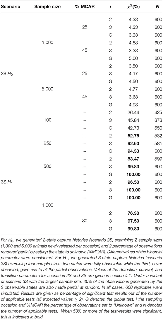
Table 5. Testing the mixture property of partial observations: simulation results.

In order to examine how the test would perform in the more challenging situation where some partial observations are generated by the observable states, we also examined for the sample size N = 1,000 a variant of the 3S scenario where, in addition to the partial observations corresponding to state C, 30% of the observations generated by the observable states A and B are set to partial at random (unknown state).

The simulation results show that for the datasets simulated under the null hypothesis (scenario 2S), the Type I error rate is close to 5%, whatever the percentage of partial observations. Importantly, the test showed good power for the datasets simulated under an alternative hypothesis (scenario 3S), with close to 50% of tests being significant for a sample size as small as 100 animals newly released per occasion (i.e., 500 animals altogether) and close to 100% of the global test being significant for 250 animals released per occasion. The simulation results show that the test reacts as expected from the derivation made in the previous sections, when the partial observations are not generated by the directly observable states, and that it can work well for realistic sample sizes. When part of the partial observations are generated by the observable states, the test is not as powerful as could be expected but nonetheless rejects H₀.

4.2. Canada Geese

We have shown theoretically and empirically that our test has the ability to assess whether partial observations can be adequately modeled as stemming solely from the directly observable states in a capture-recapture experiment. In this section, we apply the test to an ecological dataset, chosen so that the underlying state structure is actually known.

We use the Canada geese dataset from Hestbeck et al. (1991) which consists of 21,435 migrant geese individually marked with neck-bands and re-observed at their wintering locations each year, between 1984 and 1989 (Hestbeck et al., 1991; Rouan et al., 2009). These wintering sites constituted the states in the capture-recapture experiment: mid-Atlantic (New York, Pennsylvania, New Jersey), Chesapeake (Delaware, Maryland, Virginia), and Carolinas (North and South Carolina). Since the tables needed for the test were quite sparse, we therefore used the following pooling strategy: on the columns, pooled to the maximum until there was one degree of freedom left for the test (the column with the minimal sum is pooled with the column with the second minimal sum and so on) whilst on the rows, all the rows corresponding to mixtures are pooled so that there is just one mixture left to test for.

We examine the Canada geese dataset under both the null and alternative hypotheses by artificially creating these situations within the data. First, in order to create partial observations generated by the observable states (H₀), we set some observed geese's states to unknown (MCAR). We considered varying percentages to see how the test reacts to the amount of partial observations: 15, 25, and 45%. These situations are respectively denoted by MCAR15, MCAR25, and MCAR45 in Table 6. Then we examine situations that come under the alternative hypotheses (H₁) by setting all of the observations from a particular state to “unknown” so that this particular state becomes unobservable while the states remaining observable do not generate any partial observations. We considered two situations: all observations in state 2 are set to “unknown” (situation 2PO), or all those in state 3 are set to “unknown” (situation 3PO). Eventually, we considered the hybrid situation where, in addition to the partial observations generated by the unobservable state 3 as in scenario 3PO, 25% then 45% of the observations generated by state 2 are also set to partial: scenarios Hyb25 and Hyb45.

TABLE 6

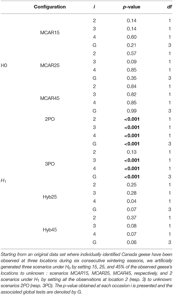
Table 6. Using different configurations of the Canada geese dataset to assess the performance of the new mixture test for assessing the underlying state structure of partial observations, under real-life conditions.

The p-values obtained from applying the mixture test to all these configurations of the geese dataset are given in Table 6. These results are very promising, with the test reacting as it should under the different configurations examined. Under all the null hypothesis configurations, the directly observable states as sole underlying states for the partial observations, there is insufficient evidence to reject the null hypothesis. For the configurations under the alternative, the null hypothesis is strongly rejected, with p < 0.001 for almost all of the tests examined (by occasion and global). The non-significant test at occasion 2 under scenario 3PO is due to the small number of individuals captured in state 3 at this occasion, resulting in insufficient power to detect the different properties of that state. Hence, the results from configurations 2PO and 3PO lead to the conclusion that the directly observable states do not provide an adequate underlying state-structure for the partial observations. When some partial observations are generated by the observable states (Hyb25 and Hyb45), there is a clear loss of statistical power. The global tests are still very close to significance at the 5% level, but more than 5 years of study would have been necessary to detect the presence of the third unmonitored location.

5. Discussion

We have derived a mixture test that assesses whether partial observations in a capture-recapture study are generated solely from the directly observable states. This test is based on distributional properties which we have demonstrated. It has been shown to perform well in theory, through simulation and for real-data applications. Regarding the interpretation of the test, if the null hypothesis is not rejected, the observable states provide an adequate underlying structure for the partial observations. However, similarly to classical goodness-of-fit tests, the interpretation of a significant test result is not as straightforward as the range of alternatives to be considered is quite large. For example, if the set of observable states are inadequate, it is not known how many additional states should be considered for the underlying structure and how the partial observations should be modeled. Both of these questions do not have obvious answers at this stage and constitute an area of future research.

Partial observations might also stem from alternatives less extreme than those considered in our applications: they could be generated by one of the directly observable states and an additional state that is never observable directly. Going further, they may also stem from all the observable states and another state which is never observable directly. In theory, the test will react to this situation too. However, in practice, we surmise that the other state would have to present different enough properties from the directly observable states for the test to be powerful enough to detect it.

Finally, determining a minimum sample size for which the test is powerful enough is more complex than usual in this framework, as it is not only the total sample size which matters but also the proportion of partial observations, which will depend on combinations of the parameter values. From a modeling perspective, we would recommend fitting a model with one additional state when the test is found to be significant.

This new test has sound theoretical basis, we showed it can work well even with small sample sizes, and we believe that it will be useful in a multi-state capture-recapture model, in statistical ecology and also other areas of application. Hidden Markov models are used for a range of purposes in capture-recapture modeling, (see for example Langrock and King, 2013; Worthington et al., 2019; Zhou et al., 2019), and the work of this paper will considerably contribute to the theoretical tools available for a wide range of applications. It will enable practitioners to consider better fitting models and will also give practical insight as to the existence of at least one state where the animals go, that is different from those directly observed.

Clearly it is desirable to consider whether the approach presented in this paper can be extended to other applications of HMMs in ecology, for example in application to movement models (Langrock et al., 2012), and beyond, and this is a current area of research.

Data Availability Statement

The canada Geese data set used as an application in this study are included in the article/Supplementary Material. The R code used to compute the sufficient statistics and the test for partial observations described in this paper are also included in the Supplementary Material. Further inquiries can be directed to the corresponding author/s.

Author Contributions

RM and RP conceived of the presented idea. AJ developed the theory and performed the computations. RP verified the theory and analytical results. All authors discussed the results and contributed to the final manuscript.

Funding

RM was funded by NERC fellowship grant NE/J018473/1 when conducting the research of this paper and by EPSRC grant EP/S020470/1 during the writing of it. AJ was funded by the School of Mathematics, Statistics, and Actuarial Science of the University of Kent (UK) and National Centre for Statistical Ecology EPSRC/NERC grant EP/I000917/1.

Conflict of Interest

The authors declare that the research was conducted in the absence of any commercial or financial relationships that could be construed as a potential conflict of interest.

Acknowledgments

We would like to thank Olivier Gimenez for letting us use part of his R code from his R2UCare package: https://github.com/oliviergimenez/R2ucare/tree/master/R.

Supplementary Material

The Supplementary Material for this article can be found online at: https://www.frontiersin.org/articles/10.3389/fevo.2021.598325/full#supplementary-material

Presentation. Supplementary Material.

Data Sheet S1. CSV: Canada Geese dataset.

Data Sheet S2. ZIP: R code to compute the sufficient statistics and the test described in the paper.

References

Bartolucci, F., and Pennoni, F. (2007). A class of latent Markov models for capture- recapture data allowing for time, heterogeneity and behavior effects. Biometrics 63, 568–578. doi: 10.1111/j.1541-0420.2006.00702.x

PubMed Abstract | CrossRef Full Text | Google Scholar

Cormack, R. M. (1964). Estimates of survival from sighting of marked animals. Biometrika 51, 429–438. doi: 10.2307/2334149

CrossRef Full Text | Google Scholar

Cressie, N., and Read, T. R. C. (1984). Multinomial goodness-of-fit tests. J. R. Stat. Soc. Ser. B Methodol. 46, 440–464.

Google Scholar

Cressie, N., and Read, T. R. C. (1988). Goodness-of-Fit Statistics for Discrete Multivariate Data. New York, NY: Springer.

Google Scholar

Hestbeck, J. B., Nichols, J. D., and Malecki, R. A. (1991). Estimates of movement and site fidelity using mark-resight data of wintering Canada geese. Ecology 72, 523–533. doi: 10.2307/2937193

CrossRef Full Text | Google Scholar

Kendall, W. L. (2004). Coping with unobservable and mis-classified states in capture-recapture studies. Anim. Biodiver. Conserv. 27, 97–107. Available online at: http://abc.museucienciesjournals.cat/files/ABC-27-1-pp-97-107.pdf

Google Scholar

King, R., and McCrea, R. S. (2014). A generalised likelihood framework for partially observed capture–recapture–recovery models. Stat. Methodol. 17, 30–45. doi: 10.1016/j.stamet.2013.07.004

CrossRef Full Text | Google Scholar

Langrock, R., and King, R. (2013). Maximum likelihood estimation of mark-recapture-recovery models in the presence of continuous covariates. Ann. Appl. Stat. 7, 1709–1732. doi: 10.1214/13-AOAS644

CrossRef Full Text | Google Scholar

Langrock, R., King, R., Matthiopoulos, J., Thomas, L., Fortin, D., and Morales, J. M. (2012). Flexible and practical modeling of animal telemetry data: hidden Markov models and extensions. Ecology 93, 2336–2342. doi: 10.1890/11-2241.1

PubMed Abstract | CrossRef Full Text | Google Scholar

Lebreton, J. D., Nichols, J. D., Barker, R. J., Pradel, R., and Spendelow, J. A. (2009). Modeling individual animal histories with multistate capture-recapture models. Adv. Ecol. Res. 41, 87–173. doi: 10.1016/S0065-2504(09)00403-6

CrossRef Full Text | Google Scholar

Moore, D.S. (1986). “Tests of chi-squared type,” in Goodness-of-Fit Techniques, eds R. B. D'Agostino and M. A. Stephens (New York, NY: CRC Press). 63–96.

Otis, D. L., Burnham, K. P., White, G. C., and Anderson, D. R. (1978). Statistical inference from capture data on closed animal populations. Wildl. Monogr. 62, 1–135.

Pledger, S. (2000). Unified maximum likelihood estimates for closed capture recapture models using mixtures. Biometrics 56, 434–442. doi: 10.1111/j.0006-341x.2000.00434.x

PubMed Abstract | CrossRef Full Text | Google Scholar

Pohle, J., Langrock, R., van Beest, F. M., and Schmidt, N. M. (2017). Selecting the number of states in hidden Markov models: pragmatic solutions illustrated using animal movement. J. Agric. Biol. Environ. Stat. 22, 270–293. doi: 10.1007/s13253-017-0283-8

CrossRef Full Text | Google Scholar

Pradel, R. (2005). Multievent: an extension of multistate capture-recapture models to uncertain states. Biometrics 61, 442–447. doi: 10.1111/j.1541-0420.2005.00318.x

PubMed Abstract | CrossRef Full Text | Google Scholar

Pradel, R., Wintrebert, C. M. A., and Gimenez, O. (2003). A Proposal for a goodness-of-fit test to the Arnason-Schwarz multisite capture-recapture model. Biometrics 59, 43–53. doi: 10.1111/1541-0420.00006

PubMed Abstract | CrossRef Full Text | Google Scholar

Rouan, L., Choquet, R., and Pradel, R. (2009). A general framework for modeling memory in capture-recapture data. J. Agric. Biol. Environ. Stat. 14, 338–355. doi: 10.1198/jabes.2009.06108

CrossRef Full Text | Google Scholar

Williams, B. K., Nichols, J. D., and Conroy, M. J. (2002) Analysis and Management of Animal Populations. San Diego, CA: Academic Press.

Google Scholar

Worthington, H., McCrea, R. S., King, R., and Griffiths, R. A. (2019). Estimating abundance from multiple sampling capture-recapture data via a multi-state multi-period stopover model. Ann. Appl. Stat. 13, 2043–2064. doi: 10.1214/19-AOAS1264

CrossRef Full Text | Google Scholar

Yang, H. C., and Chao, A. (2005). Modeling animals behavioral response by Markov chain models for capture-recapture experiments. Biometrics 61, 1010–1017. doi: 10.1111/j.1541-0420.2005.00372.x

PubMed Abstract | CrossRef Full Text | Google Scholar

Yantis, S., Meyer, D. E., and Smith, J. K. (1991). Analyses of multinomial mixture distributions: new tests for stochastic models of cognition and action. Psychol. Bull. 110, 350–374. doi: 10.1037/0033-2909.110.2.350

PubMed Abstract | CrossRef Full Text | Google Scholar

Zhou, M., McCrea, R. S., Matechou, E., Cole, D. J., and Griffiths, R. A. (2019). Removal models accounting for temporary emigration. Biometrics 75, 24–35. doi: 10.1111/biom.12961

PubMed Abstract | CrossRef Full Text | Google Scholar

Zucchini, W., MacDonald, I. L., and Langrock, R. (2016). Hidden Markov Models for Time Series: An Introduction Using R. Boca Raton, FL: Chapman and Hall; CRC Press.

Google Scholar