A Systematic Review of Within-Population Variation in the Size of Home Range Across Ungulates: What Do We Know After 50 Years of Telemetry Studies?

Studying the factors determining the sizes of home ranges, based on body mass, feeding style, and sociality level, is a long-standing goal at the intersection of ecology and evolution. Yet, how species-specific life history traits interact with different components of the landscape to shape differences in individual home ranges at within-population level has received much less attention. Here, we review the empirical literature on ungulates to map our knowledge of the relative effects of the key environmental drivers (resource availability, landscape heterogeneity, lethal and non-lethal risks) on the sizes of individual home ranges within a population and assess whether species' characteristics (body mass, diet, and social structure), account for observed variation in the responses of the sizes of individual home ranges to local environmental drivers. Estimating the sizes of home ranges and measuring environmental variables raise a number of methodological issues, which complicate the comparison of empirical studies. Still, from an ecological point of view, we showed that (1) a majority of papers (75%) supported the habitat productivity hypothesis, (2) the support for the influence of landscape heterogeneity was less pervasive across studies, (3) the response of cattle-type to variation in food availability was stronger than the response of moose-type, and (4) species-specific body mass or sociality level had no detectable effect on the level of support to the biological hypotheses. To our surprise, our systematic review revealed a dearth of studies focusing on the ecological drivers of the variation in the sizes of individual home ranges (only about 1% of articles that dealt with home ranges), especially in the later decade where more focus has been devoted to movement. We encourage researchers to continue providing such results with sufficient sample sizes and robust methodologies, as we still need to fully understand the link between environmental drivers and individual space use while accounting for life-history constraints.

Introduction

How the size of a home range responds to environmental changes has been the focus of many empirical studies across taxa (“home range,” singular or plural, returns 12,389 hits as a Topic on Web of Science Core Collection by 24 Nov 2020) including many studies on ungulates. Finding the drivers of variation in the sizes of home ranges within a given species across different habitats would indeed allow understanding higher-level processes such as population range expansion and restriction in the context of global changes. The size of an individual's home range (sensu Burt, 1943; i.e., “area traversed by the individual in its normal activities of food gathering, mating, and caring for young”) should adjust to the different components of the environment, as a result of the movements and habitat selection by this individual (Van Moorter et al., 2016). The relationship between the size of a home range and food resources, which corresponds to the habitat productivity hypothesis proposed by Harestad and Bunnel (1979), is expressed as:

$\begin{array}{ll}H=R/P& (1)\end{array}$

with H the size of the home range, R the overall energy requirements of an individual of a given mass (in kilocalories (kcal) per day) and P the rate of usable energy (kcal per day per unit area). Nonetheless, this formulation does not account explicitly for resources other than food (e.g., water, shelter), for avoidance of risk of death, or for social interactions. As habitats are heterogeneous (e.g., Wiens et al., 1985), the size of a home range should also depend on the spatial distribution of the amount and quality of resources (Mitchell and Powell, 2004). This was explicitly mentioned by Harestad and Bunnel (1979) but simply as an allometric constraint of large animals forced indirectly to include non-resource habitats within their home range because of the need to forage over large areas to satisfy all energy requirements. With highly dispersed resources, interstitial patches connecting food plots occur in the habitat matrix. This leads to increased exploitation costs for individuals, hence to a need for larger home ranges (Péron, 2019). While a home range with highly dispersed food patches can still be perceived by an individual as being of high quality (Mitchell and Powell, 2008), the expected relationship between classic estimates of the size of a home range (Laver and Kelly, 2008) and resources within the home range would appear negative. Furthermore, not only food resource distribution matters. Animals also face lethal risks (hunting, predation, and vehicle collision) and non-lethal disturbances perceived as risks (human presence in nature for other reasons than hunting; Ciuti et al., 2012; Berger-Tal and Saltz, 2019) that vary in space and time. These lethal and non-lethal risks generate the so-called landscape of fear (Laundré et al., 2001), which can lead to changes in the sizes of home ranges through, for instance, the need to include more refuge areas (Taylor, 1988; Powell et al., 1996). Lastly, when habitats ensuring different functions (Dunning et al., 1992; Camp et al., 2013) are far from each other, home ranges should increase to include all these habitats. Therefore, the habitat productivity hypothesis (Harestad and Bunnel, 1979), which is only based on food resources for a given mass, appears to be too restricted. Within a population, the relationship between the sizes of home ranges and environmental variables should indeed result from the interplay of individual responses to all types of resources and risks and to landscape heterogeneity. Exploring the complexity of these responses has been the goal of modeling and simulation endeavors (Moorcroft et al., 1999; Mitchell and Powell, 2004; Börger et al., 2008; Buchmann et al., 2013), paralleling the upsurge of empirical studies. After five decades of technological improvements (Wilson et al., 2008; Kays et al., 2015), it is timely to evaluate whether empirical knowledge acquired on a panel of diverse species and environments support hypotheses about the ecological drivers of the size of an individual's home range.

For a given ecological context, the sizes of home ranges should differ among individuals of different species in relation to body mass and life history tactics (Ofstad et al., 2016). Hence, the overall responses of the sizes of home ranges to changes in environmental features across individuals within a population are framed within these species-specific constraints. The main constraints should result from body mass, which determines energy requirements (see, e.g., Robinson et al., 1983) and the potential distance covered during a unit of time (at least within a taxonomic group), and to life style, which determines resource acquisition (Dobson, 2007). As metabolic rates are hypo-allometrically scaled with body mass, large individuals need less food per mass unit than small ones, so that R in Equation 1 scales with an allometric exponent of ca. 0.75 (Brody, 1945) and are also less selective in terms of food quality than small ones (Demment and Van Soest, 1985). In addition, as habitat features are independent of species size, the available energy per area does not change with body mass (Jetz et al., 2004) but the rate of acquisition does, which leads P in Equation 1 to have the dimension of frequency (with an allometric exponent close to −0.25, e.g., Robinson et al., 1983). This difference in allometric exponents leads the size of a home range for a given resource requirement to decrease much faster with increasing resource availability in large than in small individuals, and thereby to expect the decrease of the size of an individual's home range with increasing P to be weaker in small than in large species.

Among lifestyle traits that determine resource acquisition, diet is of prime importance (Searle and Shipley, 2008) and strongly influences the sizes of home ranges across mammals (Harestad and Bunnel, 1979; Tucker et al., 2014). Ungulates are mostly herbivores with a generalist diet, but they differ in their morpho-physiological characteristics, which cascades into how flexible their diet can be. Codron and Clauss (2010) distinguished species with a “moose-like” rumen, which have a suit of morpho-physiological features that restrict them to feed on browse material, and species with a “cattle-like” rumen, which allows them to have a more flexible diet. Individuals of species with moose-type rumen should therefore be more sensitive to variation in resource availability than individuals with cattle-type rumen, which have a wider diet niche (Codron and Clauss, 2010). In addition, as browse material represents more sparsely distributed resources (Jarman, 1974; Gordon, 2003), the sizes of home ranges of individuals with moose-type rumen, which are browsers, should be most sensitive to changes in landscape heterogeneity.

Studies performed across species have long pointed out that the sizes of home ranges should also vary with home range overlap among individuals (Jetz et al., 2004; Péron, 2019), and then according to the average group size typical of a species (Damuth, 1981; Mcloughlin et al., 2000). Hence, the size of an individual's home range for a given resource availability should be larger in group-living individuals than in solitary individuals. In populations with diverse group sizes (a common feature of group-living ungulates, Prox and Farine, 2020), the variation in the number of individuals sharing home ranges should weaken the influence of resource availability on the sizes of home ranges.

One last aspect to consider for identifying the relative roles of resources, landscape heterogeneity, and lethal and non-lethal risk on the sizes of home ranges is the seasonality of the resources, as ungulate populations face a succession of productive and non-productive seasons. The signature of food resources on the sizes of home ranges should therefore be stronger in the limiting than in the productive season (Volampeno et al., 2011), even though this effect could be dampened in some species by the ability of individuals to acquire fat reserves during the productive season, allowing them to cope with a limited access to resources during the lean season (Mautz, 1978; Stephenson et al., 2020).

Based on a systematic literature review of the variation in the sizes of individual home ranges at the within-population level in ungulates, we aimed at assessing (1) the empirical support for an impact of the different ecological drivers (resource availability, landscape heterogeneity, and lethal or non-lethal risk) on the size of an individual's home range and (2) whether the level of support found in the different publications depended on the lifestyle traits (body mass, diet, and social structure) of the species studied. Ungulates occupy all biomes, are central in terrestrial trophic networks (Montgomery et al., 2019), display a large range of both body mass and ecological traits (Fritz and Loison, 2003), and have been the focus of studies on the sizes of home ranges at the individual, population, and species levels since the 1970s (e.g., McNab, 1963; Estes, 1974; Jarman, 1974; Dunn and Gipson, 1977; Owen-Smith, 1977). Thus, ungulate home ranges have been studied by direct observation for decades and by the use of telemetry from the early days of its development for wildlife (e.g., Dunn and Gipson, 1977). Collars with VHF and now GPS and biologgers (Kays et al., 2015) have been deployed on an ever-growing number of species, providing a rich literature on the sizes of home ranges (for interspecific overviews, see, e.g., Mysterud et al., 2001; Ofstad et al., 2016). Yet, to map the determinants of the sizes of home ranges among individuals across species, methodological questions arise about how the sizes of home ranges are estimated from location data, and how environmental variables are measured (Nilsen et al., 2005). These are not trivial issues as attested by the substantial literature focusing on the meaning and definition of a home range (Kie et al., 2010; Fieberg and Börger, 2012; Powell and Mitchell, 2012; Péron, 2019), as well as on statistical methods to estimate not only the sizes of home ranges (Börger et al., 2006a; Kie et al., 2010; Noonan et al., 2019; Péron, 2019) but also resource availability (from the field, Flombaum and Sala, 2007; Redjadj et al., 2012; or remotely, Pettorelli et al., 2005, 2006; Garroutte et al., 2016; and more specifically, the edible portion of the biomass, Duparc et al., 2020) and landscape heterogeneity (Sundell-Turner and Rodewald, 2008).

In the midst of these ecological and methodological challenges, we reviewed the empirical support for the impact of three main ecological drivers (resources, landscape heterogeneity, and risks), on the variation in the sizes of individual home ranges, accounting for article-specific confounding methodological variables (sample size, positioning system, number of locations, number of metrics considered, home range estimator). Comparing the results across all articles, we then tested whether the effect of resources on the sizes of home ranges was supported more pervasively during the productive than during the non-productive season. Furthermore, we checked whether lifestyle traits such as body mass, group size and diet explained the level of support to the ecological hypotheses found in published articles (Figure 1). After mapping the state of our knowledge after five decades of upsurge in the number of studies on the sizes of home ranges in ungulates, and in times when new technologies revolutionize the fine-scale monitoring of animal movement and behavior (Wilson et al., 2008, Kays et al., 2015), we identify the remaining challenges and raise guidelines for future studies.

FIGURE 1

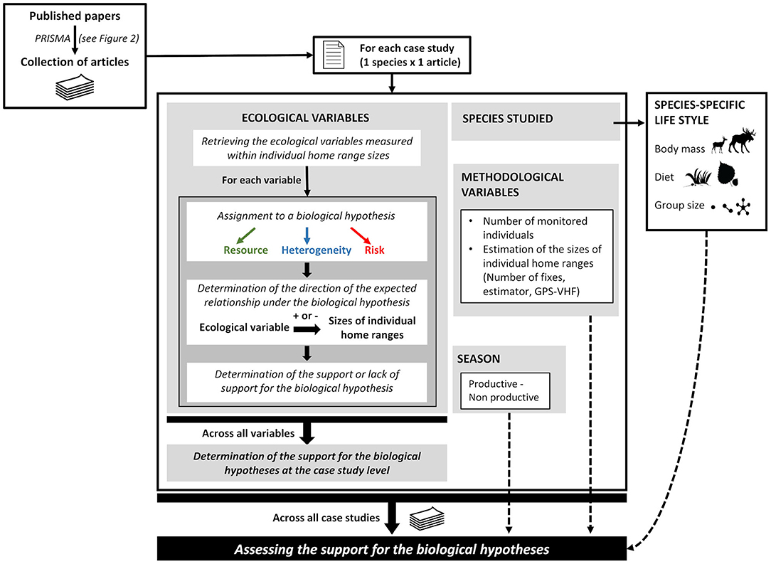
Figure 1. Schematic summary of the methodological framework. We tested biological hypotheses derived from a review of the empirical literature regarding (1) the ecological drivers of the sizes of individual home ranges (resource, landscape heterogeneity, and risk) and how (2) species-specific lifestyle traits (body mass, group size, and diet) and (3) seasonal resource variation (productive vs. non-productive season) impact the level of support to each hypothesis, while taking into account methodological variables. Each article was assessed to determine whether the relationship between the sizes of individuals' home ranges and the ecological metrics were consistent with hypotheses about the ecological drivers. The results in the article were considered supporting the hypothesis concerning ecological drivers if at least one metric was retained. The probability to support a hypothesis was evaluated using the data collected across all case studies from the review. Pictograms downloaded from http://www.phylopic.org or from the personal collection of authors.

Materials and Methods

Literature Survey

We conducted the literature survey using the Web of Science Core Collection, and then applied the PRISMA procedure (Liberati et al., 2009, Figure 2) to select a collection of comparable papers (Figure 1). We used the following keywords (“home range" OR “range use” OR “spatial distribution” OR “space use” OR “spatial variation” OR “area use” OR “habitat use” OR “ranging behavio^*”) AND (“ungulate^*” OR “herbivore^*” OR “mammal^*” OR “deer” OR “chamois” OR “ibex” OR “mouflon” OR “bison” OR “capreolus”) and obtained a total of 7,454 articles (Figure 2). We deliberately added a few names of species as keywords to incorporate older studies, which usually used the name of species in titles or keywords instead of broader taxonomic (e.g., ungulates) or ecological (e.g., herbivores) terms. We restricted the results of our search to the topics Ecology, Zoology, Environmental, and Behavioral sciences. The survey included articles published up to October 2019. Our selection followed three steps (Figure 2). We first retained for further consideration only articles for which data on the sizes of home ranges were provided for ungulates and at the population level. We restricted our review to herbivorous ungulates, hence removing articles on the wild boar (Sus scrofa), an omnivorous species, but included articles on elephant (Loxondonta africana), which is an herbivorous subungulate. This led us to keep 216 articles out of the 7,454. Second, we retained only articles providing a continuous relationship between the sizes of individual home ranges and an independent ecological metric measured at the individual home range level. This led us to remove 165 and retain 53 articles. Two of the discarded articles (Börger et al., 2006b on roe deer, Capreolus capreolus, and Brook, 2010 on elk, Cervus canadensis) provided the sizes of home ranges for individuals assigned a priori to habitat categories defined by their dominant vegetation type, which were synthetic proxies of differences in all ecological drivers (resource, landscape heterogeneity, risk). We could therefore not derive results concerning the relationship between the size of an individual's home range and an ecological metric of resource, landscape heterogeneity or risk from these articles that would compare with the other retained articles. Third, we considered only articles that provided the sizes of seasonal home ranges to test the hypothesis that the expected effect of resources on the sizes of individual home ranges should get more support during the non-productive than during the productive season. Although we recognize that there are several meanings and definitions of home range in the literature (see introduction), here we have had to accept by default the definition adopted by the authors in each of the selected studies.

FIGURE 2

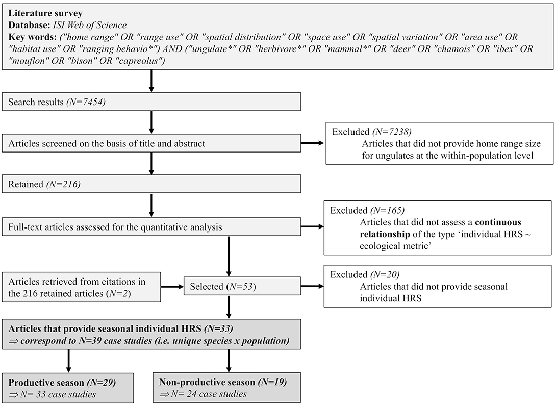
Figure 2. PRISMA flow diagram, according to the PRISMA statement by Liberati et al. (2009) and recommended by Nakagawa and Poulin (2012).

Literature Analysis and Retrieval of Article and Species Metadata

For each retained article, we started by recording the basic information required to identify each article (i.e., title, first author, year of publication, journal), the species studied and study sites. When an article considered several species or several study sites, we split it accordingly, as our unit of interest for retrieving the environmental-to-home range relationship was the species-specific population. Then, we called a “case-study” each unique species-population, which became our unit of study. We retrieved data related to animal sampling (sample size, age, and sex), duration and period of monitoring (e.g., all year round, during which season) (Table 1). We also recorded information about the location data: type of collars used (VHF or GPS) and number of fixes used per animal to estimate the size of its home range. Then, we classified each paper according to the method used to estimate the sizes of home ranges [Minimum Convex Polygon (MCP), Kernel Density Estimation (KDE), Local Convex Hull (LoCoH), Harmonic Mean (HM), and Brownian Bridge (BB)], thereafter regrouped into three classes: MCP, KDE vs. other methods for further analysis. We also classified papers according to time frame (i.e., day, week, month, season, or year), and spatial scale in terms of isopleths (e.g., 50 or 90% of utilization distribution). We discarded estimates at a time frame lower than 1 month, because the ecological meaning of very short-term home ranges is debatable (Péron, 2019), and at annual time frame because we were interested to test the impact of seasonal variation in resources on the support of ecological drivers. It is worth noting that the few articles estimating the sizes of home ranges at the day or week levels also provided estimates at a longer time frame, so we did not discard any case study for this reason. We did not retain sizes of home ranges estimated with <70% of locations.

TABLE 1

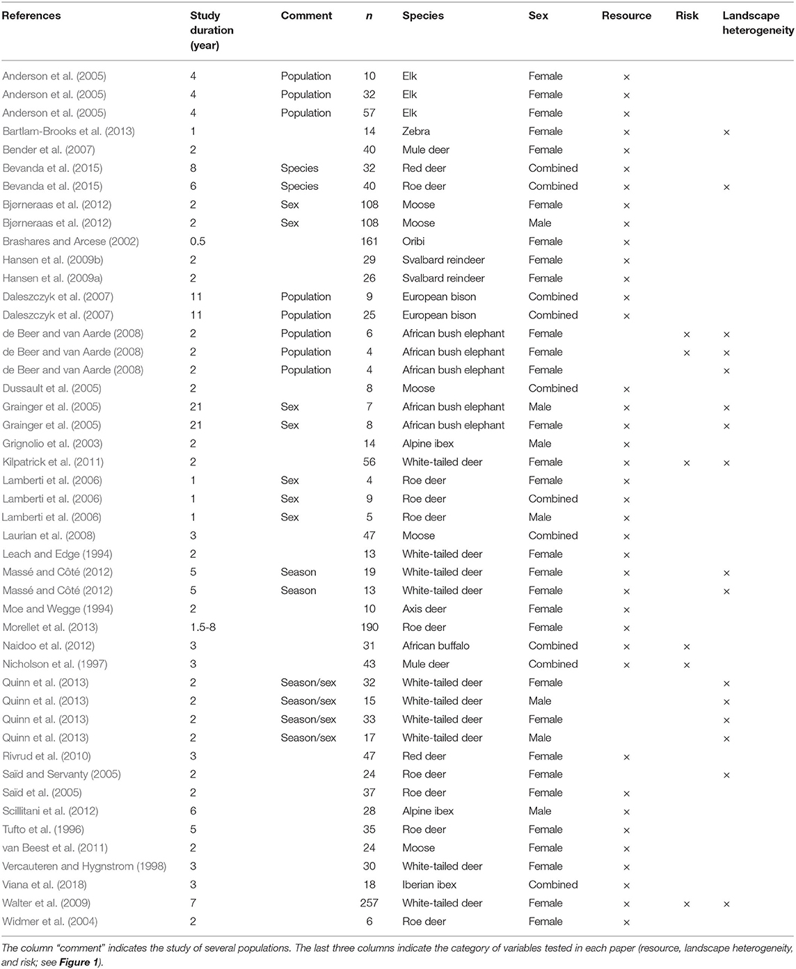
Table 1. Information on the 33 selected papers (productive and non-productive seasons).

As a second step, we listed all the ecological variables studied in a case study. For each of these variables, we retrieved the unit of measurement, the spatial scale at which it was estimated (e.g., at the home range scale or in a buffer around the home range), and whether it was log-transformed before being included in the analyses. Indeed, the relationship between the sizes of home ranges and productivity becomes linear only when both of them are log-transformed (Equation 1). We faced a huge diversity of metrics (Supplementary Table 1), which we classified as measures of resource, landscape heterogeneity, or risk (Figure 1; Supplementary Table 1). We then counted the number of metrics for a given category of variables (resource, landscape heterogeneity, risk) and a given season (productive and non-productive season) studied per case study. We did not consider the following metrics: index of snow severity (Ramanzin et al., 2007), snow cover (Grignolio et al., 2003), snow depth (van Beest et al., 2011; Scillitani et al., 2012), elevation (Hansen et al., 2009a; Bevanda et al., 2015), and slope (Anderson et al., 2005), since these factors were only relevant to some specific environments (e.g., mountainous and arctic regions). Based on the species' ecology and information given in each article, we associated each metric to the expected slope direction of its relationship with the sizes of home ranges: increase, i.e., positive effect size, or decrease, i.e., negative effect size. For example, to be in line with the resource hypothesis, we expected a negative relationship between the sizes of individual home ranges and resource metrics reflecting good quality forage (e.g., grass nitrogen content, Brashares and Arcese, 2002), but a negative relationship when resource metrics were related to poor-quality forage (e.g., fiber content, Brashares and Arcese, 2002).

As a third step, we retrieved species-specific traits from the literature, such as adult body mass for both sexes, type of physio-digestive system (moose-type vs. cattle-type), sociality level, and phylogenetic information (see Table 2). We did not use phylogenetic information in our models due to the low number of species (15 species) finally retrieved in our sample (see “Results” section). For ranking species on the generalist-specialist gradient, we used the type of physio-digestive system (moose-type vs. cattle-type), as proposed by Codron and Clauss (2010). For the social structure, we classified species as living in small groups (solitary to small groups up to five individuals) and in large groups (six or more), following the classification proposed by Prox and Farine (2020).

TABLE 2

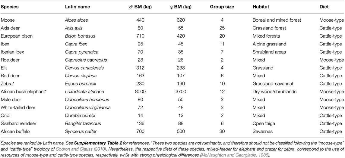
Table 2. Characteristics of the species included in the 33 selected papers (productive and non-productive seasons).

Extraction of Results

In the retained articles, independent variables were considered to influence the sizes of home ranges either based on an information theory approach [usually comparing models with an information criterion, such as Akaike Information Criterion (AIC)] or by inferential procedures based on statistical tests and p-values. Retrieving standardized effect sizes required for a meta-analysis was not possible because independent variables were mostly included in multivariable models, were not systematically scaled or log-transformed, and statistics needed to calculate effect sizes were not all (or not at all) provided in the article (especially for variables found to have no statistically significant effect or that were not included in the best models). Consequently, we summarized the results in a categorical way instead of reporting the estimated values of effect sizes (i.e., slopes and standard errors). For each metric (Figure 1), we recorded, whether the analyses reported in the article supported our biological hypotheses regarding resource, landscape heterogeneity, or risk, i.e., whether the relationship between the sizes of home ranges and the ecological variable was in the same direction as expected, in the opposite direction, or not retained. For independent variables without detectable effect or not included in the selected model, we sought whether the slope was nevertheless in the expected direction, or opposite to the expected direction, when given. Therefore, we ended up with variables assigned to five different result categories: “as expected and detected or retained in the best models”, “as expected and not detected or not retained in the best model”, “opposite and detected or retained in the best model”, “opposite and not detected or not retained in the best model”, or “direction unknown and not detected or not retained in the best model”. The distribution of the five different categories of results is provided in Supplementary Figure 1. For the rest of our analyses, we classified the result of each metric as being supporting, or not supporting, the biological hypothesis it was assigned to Figure 1. Importantly, we considered that a biological hypothesis was supported in a case study if at least one of its metrics was supporting the given biological hypothesis, independently of the number of metrics tested. We are aware that a statistical hypothesis can only be rejected or not rejected, but for greater clarity throughout the manuscript, we use the terms “supporting” the biological and ecological hypothesis tested for “rejecting” the null statistical hypothesis, and “not supporting” the biological and ecological hypothesis tested for “not rejecting” the null statistical hypothesis.

Descriptive and Statistical Analysis

We performed an in-depth analysis of the probability for a study to support each of the biological hypotheses. Using generalized linear models (GLMs), we first tested whether methodological covariables influenced the probability of support for a given biological hypothesis, considered as a binomial response variable (Figure 1). The methodological variables tested were sample size (for a given expected effect size, large sample size should positively influence the likelihood to detect a relationship), the number of variables studied (the larger the number of variables considered, the more likely one would be retained), and all technical aspects expected to increase the accuracy of estimates of the sizes of individual home ranges (number of relocations; positioning system, VHF vs. GPS; statistical method used to estimate the sizes of home ranges). We then assessed if the level of support for a biological hypothesis differed for resource, landscape heterogeneity, or risk and whether it was more important for resources during the non-productive season than during the productive season. Note that due to the few case studies focusing on risk (and none on risk only), we did not include this category in models, hence we were not able to assess the level of empirical support for our hypothesis that individual exposure to risk should affect the sizes of individual home ranges. We included a two-way interaction between the ecological driver (resource and landscape heterogeneity) and the number of metrics tested, as this number was generally higher for landscape heterogeneity. We compared models accounting for methodological variables using the Akaike Information Criterion and selected the model with the lowest AIC value.

Then, we assessed whether the lifestyle variables (Figure 1) could influence the level of support to each ecological driver: body mass (expecting an increased support with increasing body mass), diet (expecting a stronger support for species with moose-type digestive features), and social structure (expecting a reduced support in large group-living species).

We fitted GLMs with a binomial distributed error structure and a logit link function, using the “glm” function implemented in the package “stats” of R 3.3.3 (R Development Core Team, 2017). We ranked candidate models using the Akaike Information Criterion for small sample sizes (AICc) as implemented in the R package “AICcmodavg” (Mazerolle, 2020) and calculated ΔAICc and AICc weights. Models with ΔAICc ≤ 2 were considered equivalent (Burnham and Anderson, 2002), and when models had a ΔAICc ≤ 2, we kept the most parsimonious one. Results are depicted using the “sjPlot” (Lüdecke, 2019) and “visreg” (Breheny and Burchett, 2017) R-packages.

Results

Studies and Species

We retained 33 articles, published in 26 different scientific journals that met our two first criteria of selection (Figure 2), covering both the productive (29 articles) and non-productive (19 articles) seasons. Most studies were published during the early 2000–2010, with a noticeable decrease post-2013 (Figure 3A). Fifteen species were studied during at least one of the productive and non-productive seasons (Figure 3B). These species belong mostly to the order Artiodactyla, and are essentially members of the families Bovidae (five species) and Cervidae (eight species)—the remaining two species belong to the Equidae (Equus burchelli) and Elephantidae (Loxodonta africana) (Figure 3B). Among these species, some have been studied more than others, as 19 of the 33 articles (57%) focused on only three species: roe deer Capreolus capreolus (eight articles), white-tailed deer Odocoileus virginianus (seven articles), and moose Alces alces (four articles). Individuals from different species were contrasted in terms of body mass, group size, habitat, and percentage of grass in the diet (mean = 45.9 ± 29.5): six species were classified as having individuals forming low group sizes and nine as having highly social individuals (Table 2).

FIGURE 3

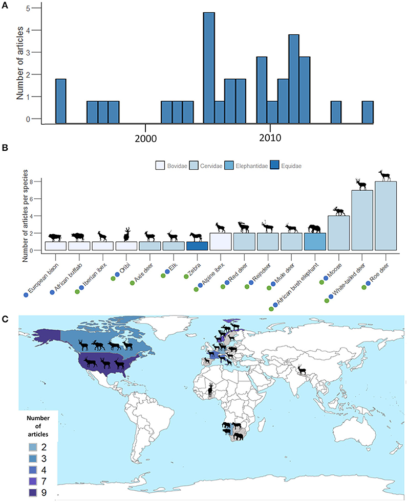
Figure 3. (A) Number of articles published each year. (B) Number of articles per species. Dots depict species for which we were able to retrieve information on seasonal relationships between the sizes of home ranges and biomass of vegetation during the productive (green dots) and non-productive (blue dots) periods and retained in the final comparative analysis (see PRISMA; Figure 2). (C) Map of the countries where studies took place. Numbers of publications per country are indicated by different colors.

Almost all studies have been conducted in North America (n = 10) and Europe (n = 17), with only five studies located in Southern Africa (Figure 3C). We retrieved only one study conducted in Asia [axis deer Axis axis in Nepal, Moe and Wegge (1994)]. Among the 33 retained articles, three included several populations of the same species (Anderson et al., 2005; Daleszczyk et al., 2007; de Beer and van Aarde, 2008) and one article studied two species (Bevanda et al., 2015). Overall, this led to 39 independent case studies (Table 1).

Telemetry and Estimators of the Sizes of Home Ranges

Animal locations were obtained either by GPS or VHF positioning system. Before 2000, all studies used VHF collars (Figure 4A). GPS collars came into use in 2000 and dominated until after 2010 (Figure 4A). Before 2000 (five case studies), MCP dominated, and two methods (KDE and Harmonic Mean method as the only “other methods”) were used equivalently (Figure 4B). During the 2001–2010 (23 case studies), KDE took over MCP, with 63% of articles using KDE. Since 2011 (11 case studies), methods used have diversified, leading to a decrease in the occurrence of MCP and KDE. The increased use of other methods in the later years corresponded to the development of alternative home range estimators such as LoCoH or brownian bridge methods. Twenty-five case studies (65%) were based on <20 marked animals, while only six case studies (15%) had sample sizes above 50 (Figure 4C). The number of relocations used to estimate the sizes of home ranges also revealed a strong variability among the 39 case studies (Figure 4D). On average, about 852 locations per month were used to compute the sizes of home ranges, but with a wide range, with minimum and maximum numbers of locations being 6 and 5,040 locations, respectively.

FIGURE 4

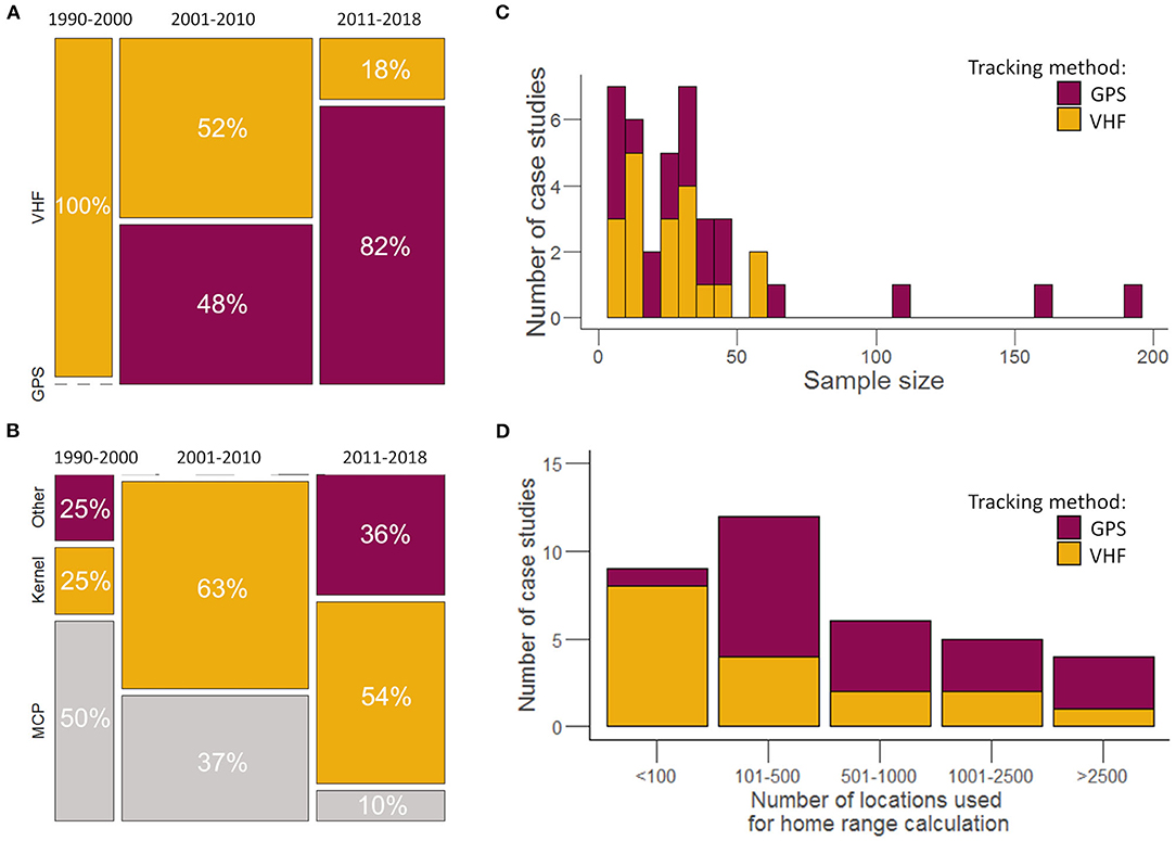
Figure 4. (A) Evolution of tracking methods used in the 33 selected articles (GPS, VHF) according to a 10-year time period. The width of the bars corresponds to the percentage of articles by time period. The percentages given in the bars represent the percentage of articles with data collected with GPS vs. VHF per time period. (B) Evolution of home range estimators used in the 33 articles according to time period. The percentages correspond to the proportions of articles per time period for each home range estimator. (C) Distribution of the number of individuals per case study (n = 39) according to tracking method. (D) Distribution of the number of locations used for home range calculation in the 39 case studies according to the tracking method.

Descriptive Summary of Studied Variables

Most case studies focused on variables related to “resource” (n = 34), followed by “landscape heterogeneity” (n = 12) and lethal or non-lethal “risk” (n = 6; Figure 5A). No case study focused solely on lethal or non-lethal risk, and this factor was always tested in conjunction with one of the other two categories of variables or with both of them. All variables considered as metrics of risk by the authors were distance or density of linear features (e.g., road) (Supplementary Table 1). The majority of case studies investigated the effect of several independent variables on the sizes of home ranges with on average 2.6 relationships tested per case study for resource (range: 1–12), 7.8 for landscape heterogeneity (range: 1–12), and 1.3 for risk (range: 1–3) (Figure 5B). As too few studies assessed the influence of lethal or non-lethal risk, this ecological driver was excluded from the analyses. We retrieved 123 slopes characterizing the link between the sizes of home ranges and resource, 152 for the category of landscape heterogeneity variables, and eight for risk metrics. Only 15 papers out of the 33 log-transformed the sizes of home ranges.

FIGURE 5

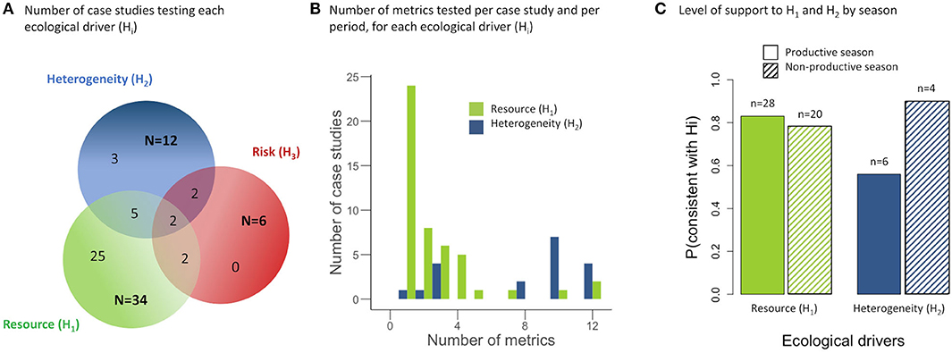
Figure 5. Venn diagrams for (A) the number of case studies testing a relationship between the sizes of home ranges and resource, landscape heterogeneity or risk indices, and combinations of these. (B) Number of metrics tested per case study, per period, and for each ecological driver. (C) Proportion of case studies that contained at least one metric supporting the biological hypothesis, for each ecological driver and season.

The results at the metric level supported one of the biological hypotheses and were detected or retained for 37% of the metrics across all studies, whereas they were opposite to the initial expectation and detected or retained for 13% of the metrics (Supplementary Figure 1). Not detected or non-retained metrics were reported for 50% of the metrics (16% were consistent and 16% opposite to the direction expected under the biological hypotheses and finally 18% were unknown, Supplementary Figure 1).

Methodological Covariables and Seasonal Variation Influencing Papers' Results

Eighty percent of the 33 case studies focusing on resource metrics (28 in the productive season and 20 in the non-productive seasons) concluded that the habitat productivity hypothesis was supported (i.e., at least one variable tested supported the expected impact of resources on the sizes of home ranges). This percentage was 73% for the 12 case studies studying landscape heterogeneity (9 in the productive season, and 10 in the non-productive seasons; Figure 5C).

The probability for a case study to support the biological hypotheses increased with sample size (β = 0.23 ± 0.30, log scale; Figure 6A) and was influenced by the two-way interaction between the number of metrics and the biological hypothesis considered (β = 1.21 ± 0.52 for resource, β = −0.07 ± 2.02 for landscape heterogeneity; Figure 6B) and by the positioning system (β_{VHF vs. GPS} = 1.51 ± 1.27; Figure 6C and see Supplementary Table 3 for details). Neither the number of locations per individual nor the estimation method of the sizes of home ranges (KDE, MCP, and others) was retained in the best models (all ΔAICc > 2; see Supplementary Table 3). When looking at the prediction from the best model, the percentage of studies supporting the expected relationship between the sizes of home ranges and resources were close to 100%, when animals were monitored by VHF or by GPS (mostly from papers after 2010, Figure 3), as long as enough resource metrics (roughly >4) were measured (Figure 6B). Landscape heterogeneity influenced the sizes of home ranges in about 96% of studies based on individuals monitored by VHF but in only about 75% for individuals monitored by GPS, whatever the number of studied metrics. Neither the season nor the interaction between season and category of variables were retained in the best model for resources (Supplementary Table 3).

FIGURE 6

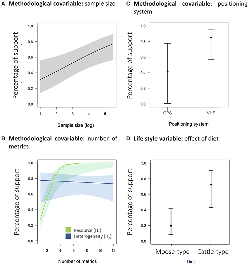
Figure 6. Effect of (A) the sample size (log-transformed; if the positioning system was GPS, the season was the non-productive season, the number of metrics was 4.07 and the ecological driver was the resource one). (B) The number of metrics tested [if the sample size was 3.06 (log-transformed), the positioning system was GPS and the season was the non-productive season] on the probability to have at least one metric supporting the biological hypotheses. These results correspond to the model that explains the probability of support for each hypothesis according to the different methodological features accounted for differences among case studies. (C) The positioning system [if the season was the non-productive one, the number of metrics was 4.07, the ecological driver was the resource one, and the sample size was 3.07 (log-transformed)]. (D) Effect of diet [if the positioning system was GPS, the sample size was 3.18 (log-transformed) and the season was the non-productive season] on the probability to have at least one metric supporting biological hypothesis. This model was performed on a subset of our sample with the resource hypothesis only and the case studies studying the two seasons. The response variable for the four panels is binomial, whereby 0 means that the authors concluded that their hypothesis was not supported, and one otherwise (see Figure 1). The shades in (A and B) correspond to the 95% confidence interval.

Influence of Species-Specific Life History Traits on Findings

We added body mass (log-transformed), group size, and diet to the baseline model selected above to test for the lifestyle-related hypotheses (Figure 1). Body mass, group size, or diet did not affect the level of support for the biological hypothesis in models where both resource and landscape heterogeneity were considered together (Supplementary Table 4). Only the variables of the baseline model (i.e., sample size, positioning system, and the two-way interaction between the number of metrics and the ecological driver) were retained.

We then focused on the metrics from the resource category only to test more specifically the resource hypothesis and whether the support for the resource hypothesis was larger in species with a moose-type than a cattle-type rumen (model selection table in Supplementary Table 5). We actually found the opposite, as the support to the resource hypothesis was larger for species with a cattle-type rumen (β = 0.81 ± 0.62; Figure 6D) than for moose-type (β = −1.48 ± 0.43).

Discussion

The size of an individual's home range should vary according to a triptych of factors composed by resources, landscape heterogeneity, and risk (Desy et al., 1990; Haskell et al., 2002; Kittle et al., 2008; Bonnot et al., 2013; Creel et al., 2014). Assessing the level of support to each of these drivers of variation in the sizes of individual home ranges from a literature review has however proven more challenging than we had anticipated, for many reasons. First, a dearth of studies provided exploitable results on the variation of the sizes of home ranges with ecological drivers (<1%). Second, methodological issues included the rampant debate on how to estimate both the sizes of home ranges and independent metrics, issues which are far from trivial. Third, the limited number of species studied and the limited geographic distribution of study sites, tied with the methodological concerns, are hurdles in our ability to test whether species-specific lifestyles explain the different sensitivity of individuals from each species to the main ecological drivers.

More Support to the Resource Than to the Landscape Heterogeneity Hypothesis

Resource metrics, especially food resources, have been studied more than metrics of landscape heterogeneity (Figure 5A). The majority of articles found that the sizes of individual home ranges were decreasing with increasing amounts of resources (Figure 5C), supporting the Habitat Productivity Hypothesis. On the other hand, support for the effect of landscape heterogeneity on the sizes of home ranges was more limited (Figure 5C). Landscape heterogeneity includes several components (local diversity, landscape complementarity, or landscape-level fragmentation; Dunning et al., 1992), each of which should be measured explicitly (Turner, 2005). The lower proportion of papers supporting that landscape heterogeneity affects the sizes of home ranges may therefore result from the difficulty to identify and measure the proper metric and scale at which it should be measured (Bevanda et al., 2015).

Study Design and Statistical Considerations

Sample Size and the Problem of Statistical Power

Articles were more likely to support the biological hypotheses when the studies included a large number of animals (Figure 6A), due to a higher statistical power (Steidl et al., 1997). Interestingly, the effect size linking environmental variables and the sizes of home ranges varied with life history traits (Figure 6D). Authors should therefore anticipate the statistical power of their study accounting for the biology of individuals of the studied species and their life history, to enhance the probability of finding an effect. Biological conclusions based on small samples should not be over-interpreted to avoid erroneous conclusions (Steidl et al., 1997). Fortunately, as the cost of telemetry collars are decreasing, we can expect the number of animals per study to increase for a given budget.

Technological Improvements and Estimates of the Sizes of Home Ranges

The technology to monitor individuals has greatly improved during the last 30 years (Kays et al., 2015) and, accordingly, the publications after 2010 rely mostly on GPS-collared individuals. GPS collars are more expensive than VHF collars but provide a larger number of predetermined fixes, which should ensure a better delimitation and estimation of the size of a home range (Laver and Kelly, 2008; Pellerin et al., 2008; Kie et al., 2010). Yet, studies relying on GPS collars supported biological hypotheses to a lower extent than studies where animals were VHF collared. A tendency to publish non-significant results to a greater extent in more recent years might account for this surprising result. In parallel to the change in technology, methods to estimate the sizes of home ranges have shifted from MCP to a large range of methods, which undermines the comparison and repeatability of studies (Laver and Kelly, 2008). While we did not detect any effect of the estimation method, the low number of case studies prevented us from testing for all interactions, leading us to interpret this finding with caution. Recent articles studying habitat selection or animal movements tend to skip providing the sizes of home ranges, focusing on smaller spatial scale movement behavior. This probably explains why, despite recent evaluation of the robustness of estimators of the sizes of home ranges (e.g., Noonan et al., 2019), we have retrieved fewer articles and data over the last few decades than we had hoped.

Environmental Variables: Their Number, Measurement, and Meaning

The large diversity of metrics used to measure resource availability and landscape heterogeneity, as well as the restricted number of variables assessing risk, were problematic (Supplementary Table 1). The few risk-related metrics interpreted by the authors to be risky were mostly landscape features (see Table 1) and almost no studies fitted our selection criteria for evaluating individual exposure to natural predation or hunting risks (Figure 1). The complexity to evaluate risk metrics at the individual level renders empirical studies of the possible effect of both lethal and non-lethal risk on the sizes of individual home ranges particularly challenging.

The proportion of relationships supporting biological hypotheses was quite low: 52% with resource metrics and only 21% with landscape heterogeneity metrics (Supplementary Figure 2). Quantifying resources that are edible for ungulates is tricky as it requires information on individual energetic requirements and nutritional state, diet, and diet selection (Duparc et al., 2020). Metrics used to measure these factors, derived from remote sensing, field measurements, and proportion of rich or poor habitat available, are often quite crude (Pettorelli, 2013), far from the species-specific foodscape (sensu Searle et al., 2007; Duparc et al., 2020). Likewise, the fragmentation perceived by an individual (Sundell-Turner and Rodewald, 2008) is difficult to measure from geographic databases where habitats are human-derived categories of land cover and would not necessarily reflect how animals perceive their surrounding landscape (Li and Reynolds, 1994; Baguette and Van Dyck, 2007). These difficulties to measure meaningful metrics may explain also why the probability for a case study to conclude opposite to the expectation (i.e., at least one metric tested contradicting the initial hypothesis) was quite high. The papers with such surprising results were mainly those with a large number of metrics tested. With the continuing increases in map resolution and the growing easiness to analyze patterns in a landscape through dedicated software and packages (e.g., Fragstats, Fourier transforms, Rocchini et al., 2013), researchers are tempted to include a plethora of variables, which is not advisable (Streiner and Norman, 2011). This problem probably explains the low proportion of variables found to be statistically significant, the high probability of obtaining at least one variable with an effect opposite to what is expected, and the ad hoc explanation of significant relationships. A better understanding of the energetic requirements, diet needs, and the multiple components of landscape heterogeneity as perceived by an individual is badly required and should be the focus of renewed empirical effort in the future.

Temporal and Spatial Scales

Seasonality

Contrary to our expectations, the influence of resources on variation in the sizes of home range was not supported to a greater extent during the non-productive than during the productive season. This result was surprising, given that most studies took place in areas with marked seasonality (Figure 3C). Environmental constraints might account for this discrepancy, as movements can be restricted during winter, especially at high latitude and high elevation, preventing the sizes of individual home ranges from responding to reduced food resources during the lean season (Rivrud et al., 2010). Moreover, the ability for some species to store fat reserves may relax the requirements to resort to immediately available food resources during the lean season (Mautz, 1978), so that an extension of the size of the home range may not be required. Hence, while seasonal expansion-contraction of the sizes of home ranges occurs in ungulates (Börger et al., 2006b; Morellet et al., 2013), among-individual variation in home range sizes does not appear to be triggered by food resources to a greater extent in the lean season.

Temporal Definition of Seasonal Period

Another reason why seasonal differences did not affect home range sizes may be that estimates of the sizes of home ranges were calculated over varying time windows. For the sake of comparison, we simply attributed a season to an estimate of the size of a home range, but this classification may itself cover various periods of time, from the peak period of productivity (i.e., within a few weeks), to the productive season on its whole (i.e., over several months). The estimates of both the sizes of home ranges (Börger et al., 2008) and the metrics of resources may vary with the time window. For instance, van Beest et al. (2011) reported that the lack of consistency in the effects of individual attributes and environmental conditions (resource and climate) on the sizes of home ranges could be due to the inadequate choice of the temporal scale (Table 3). A relevant choice of spatial and temporal scales is essential and should be suited to the biology of the species, in terms of how individuals perceive the environment (Cushman and McGarigal, 2004) and stationarity (Laver and Kelly, 2008; Péron, 2019).

TABLE 3

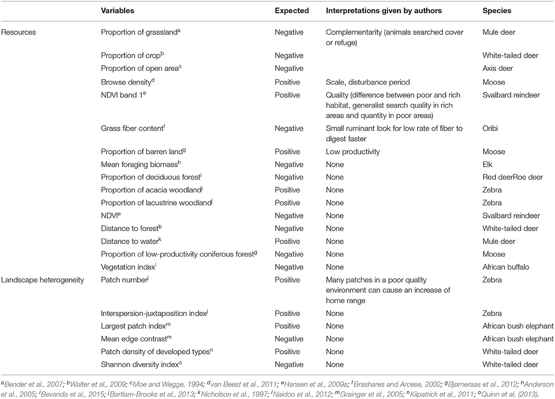
Table 3. Biological interpretations provided by authors to explain results that were retained as opposite to initial biological hypothesis, per category of variable (resource availability and landscape heterogeneity).

Accounting for Life History Traits

Body Mass

Species' body mass did not influence how the sizes of home ranges responded to environmental factors, despite the range of body mass varying from 13 to 8,000 kg, thus covering the range of body mass of ungulates (Fritz and Loison, 2003). We expected the pathways through which environmental variables cascade to the sizes of individual home ranges to be much more complex in large than small species (Haskell et al., 2002), but we did not find such evidence. In a recent paper, Noonan et al. (2020) provide evidence that investigating allometric relationship of the sizes of home ranges from conventional KDE method could be misleading as the sizes of home ranges tend to be increasingly underestimated as species body mass increases. This exemplifies that the endeavor of reviewing the variation in the sizes of home ranges requires first and foremost the development of a rigorous and accepted methodology for estimating the sizes of home ranges, while the conceptual framework is already well-anchored since the theoretical approaches developed in the late 1960s (McNab, 1963; Jetz et al., 2004).

Group Size

Unlike what we posited, the support for the biological hypotheses did not decrease in species with large group size. Our rough categories of group size at the species level and the low number of species included in our review might have prevented us from detecting the influence of group size on the relationship between resource availability or landscape heterogeneity and the sizes of home ranges. In most group-living species, the situation is complex (Prox and Farine, 2020) because groups vary in size (e.g., fission-fusion societies, Aureli et al., 2008). The lability of group sizes and also the varying degree of home range overlap among individuals of a given social unit (Mcloughlin et al., 2000) may however prevent detecting a resource-to-home range size relationship, when group size is not controlled.

Diet

The support to the resource hypothesis was higher for species with a “cattle-type” rumen (Codron and Clauss, 2010), which contradicted our expectation. This could be caused by the difficulty to obtain a reliable metric for resource availability in moose-type species (mostly browsers, Codron and Clauss, 2010), whose resources are difficult to evaluate using remote sensing. In addition, grass (consumed by individuals of species with cattle-type rumen to different degrees) produces most of its rich foliage during a limited time frame and quickly disappears when passing into the non-productive season, while browse such as ivy or bramble, due to their deep roots, can continue to produce some buds and foliage even after the end of the productive season (Jarman, 1974; Shipley, 1999). This difference in growth rates of resources can render cattle-type species to be more sensitive to resource availability. As broached earlier, a proper assessment of species-specific foodscape and of the search and exploitation balance in time budget and movements is required for a better understanding of how resource availability and landscape heterogeneity shape the sizes of home ranges in species with different diets (Shipley, 1999) and morpho-digestive constraints (Clauss et al., 2003).

Other Drivers of Variation in the Sizes of Individual Home Ranges

Individual Attributes

We only analyzed the effect of resource availability and landscape heterogeneity on the variation in the sizes of home ranges in relation to species-specific diet and group size. Nonetheless, other factors shape among-individual variation in the sizes of home ranges, such as individual attributes (e.g., sex, age, or body condition). As critical periods in terms of energetic expenditures differ between sexes (i.e., mating in males, late gestation-early lactation in females) and because females cannot move a lot after parturition, intraspecific variation in the sizes of home ranges emerges (e.g., Bowyer, 2004; Ruckstuhl, 2007). The size of an individual's home range can also vary as a function of age (Tao et al., 2016), either because individuals gain more experience and a better knowledge of resource distribution when aging (Saïd et al., 2009) or because they are increasingly less efficient at exploiting a large area (Froy et al., 2018). More generally, intraspecific variation in the internal state of individuals could lead to contrasted costs of movement (McNab, 1963) and therefore to different responses of the sizes of home ranges to changes in environmental variables.

Population Density

We omitted population density as a possible driver of the size of individual home range, as we considered population density to be an emergent property of combined individual home ranges and overlap among individuals (Damuth, 1981). Even though the sizes of home ranges can decrease with density, as shown by Kjellander et al. (2004) on roe deer, changes in home range overlap could blur this relationship (Jetz et al., 2004). More generally, a detailed appraisal of the social system should be inseparable from the study of the home range-to-density relationship (Damuth, 1981; Mcloughlin et al., 2000).

Coexisting With Other Species

In addition, most individuals share their home ranges with members of sympatric species with overlapping niches, which leads to potential competing or facilitating relationships (Buchmann et al., 2013; du Toit and Olff, 2014). Individuals living in a multispecies environment, where resources are depleted at a fast rate, should have larger home ranges than individuals living alone in a given area (Buchmann et al., 2013). The inverse may happen when facilitation occurs (du Toit and Olff, 2014). The reason the community setting is seldom considered in single-species studies of variation in the sizes of home ranges may be the strong bias of studies from the northern hemisphere, where the research tradition is more single species based, in contrast to Africa where comprehensive species and community approaches are more common (e.g., starting in the early 1970s with the works of Estes, 1974). Ungulates are also prey to various predators in all ecosystems (Montgomery et al., 2019). The impact of natural predation and human hunting on the sizes of individual home ranges within a population remains to be evaluated, accounting for both ungulate life history traits (Hopcraft et al., 2010) and predator hunting modes (cursorial vs. ambush, Say-Sallaz et al., 2019).

Recommendations

We acknowledge that in the last 15 years, several authors have reviewed in depth the concept of home range and its estimation, providing important recommendations regarding the methodology and reporting of information in published studies (for recent studies, Noonan et al., 2019, 2020; Péron, 2019). More than 10 years ago, Laver and Kelly (2008) urged researchers to follow a unified methodology for estimating animal home ranges and recommended a minimal report of information for a better reproducibility and robust comparisons among studies. Likewise, we can only insist that it would be most useful, for comparative endeavors like ours, that authors provide estimates of the sizes of home ranges obtained with different methods, if only as Supplementary Information. In addition, previous reviews provided insightful information and critical perspectives regarding the definition of a home range and the estimation of its size (Börger et al., 2008; Fieberg and Börger, 2012; Péron, 2019). In a prospective review, Börger et al. (2008) advocated for the development of a general mechanistic model of animal home range behavior that would unify movement, individual resource requirements, and statistical models of home ranges. While this review did not directly provide guidelines on how to enhance the reporting and standardization of results of home range studies, it proposed a general approach, unifying our understanding of links between small-scale movements and home range behavior. We refer the readers to these previous reviews for discussion about the concept of home range, its definition and estimation, and the future avenues of research regarding the upscaling of movements to home ranges. In our systematic review, we encountered other hurdles, such as the methodological and biological inconsistencies regarding the independent variables and the statistical models. This led us to summarize some recommendations (Table 4) that should help future empirical studies aiming at evaluating the effect of the resource availability, landscape heterogeneity, and risk on the sizes of home ranges mediated by species-specific lifestyle. These recommendations pertain to (1) study design and methodology, (2) the choice and estimation of the candidate drivers of the sizes of home ranges, although we are aware of the persistence of some challenges and disagreement across the literature on the most appropriate and meaningful metrics, for example of landscape heterogeneity, (3) general statistical considerations, and (4) the need of considering life history traits when evaluating variation in the sizes of home ranges within a population. Understanding processes at the community level requires a better grasp of how individual movements, triggered by resources, landscape heterogeneity, predation, and coexistence with other species, lead to home range formation and space sharing (Buchmann et al., 2013; Bhat et al., 2020). Our review brings to the fore that the last 50 years of telemetry studies are actually only the first steps into finding the link between environmental factors, life-history constraints, and individual space use that could feed our understanding of larger-scale processes. Therefore, we urge researchers on movement ecology to continue providing results on individual home ranges in their articles.

TABLE 4

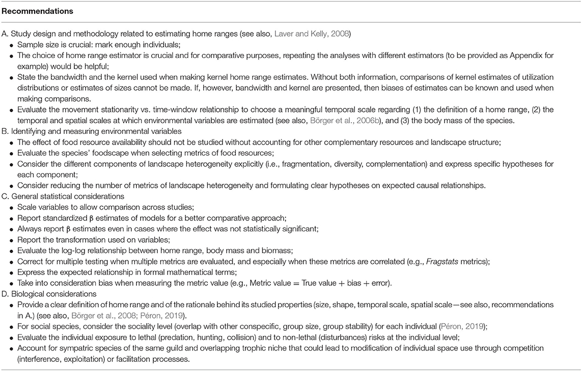
Table 4. Recommendations for authors that should help quantitative studies aiming at evaluating the effect of the environment and life history traits on the size of home range.

Data Availability Statement

The raw data supporting the conclusions of this article will be made available by the authors, without undue reservation.

Author Contributions

JS-F, KA, GY, and AL conceived this work and designed the methodology with inputs from J-MG, MG, and NM. JS-F and KA collected and analyzed the data with inputs from VR. JS-F, KA, GY, and AL led the initial writing of the manuscript. All authors contributed critically to the manuscript and gave final approval for publication.

Conflict of Interest

The authors declare that the research was conducted in the absence of any commercial or financial relationships that could be construed as a potential conflict of interest.

Acknowledgments

The study was funded by ANR grant Mov-It coordinated by A.L. (ANR-16-CE02-0010). We thank the Mov-It consortium for insightful discussions. We are also grateful to Marco Apollonio, Floris van Beest, Steeve Côté, Shunsuke Imai, Ariane Massé, Enrico Merli, Andrea Monaco, Robin Naidoo, Maurizio Ramanzin, Sonia Saïd, Laura Scillitani, Enrico Sturaro and W. David Walter for providing us with the datasets from their respective studies, and Stephen L. Webb for providing us with information on his papers. We would like to thank Roger A. Powell and John Fryxell whose comments helped improve and clarify this manuscript.

Supplementary Material

The Supplementary Material for this article can be found online at: https://www.frontiersin.org/articles/10.3389/fevo.2020.555429/full#supplementary-material

References

Anderson, D. P., Forester, J. D., Turner, M. G., Frair, J. L., Merrill, E. H., Fortin, D., et al. (2005). Factors influencing female home range sizes in elk (Cervus elaphus) in North American landscapes. Landscape Ecol. 20, 257–271. doi: 10.1007/s10980-005-0062-8

CrossRef Full Text | Google Scholar

Aureli, F., Schaffner, C. M., Boesch, C., Bearder, S. K., Call, J., Chapman, C. A., et al. (2008). Fission-fusion dynamics: new research frameworks. Curr. Anthropol. 49, 627–654. doi: 10.1086/586708

CrossRef Full Text | Google Scholar

Baguette, M., and Van Dyck, H. (2007). Landscape connectivity and animal behavior: functional grain as a key determinant for dispersal. Landscape Ecol. 22, 1117–1129. doi: 10.1007/s10980-007-9108-4

CrossRef Full Text | Google Scholar

Bartlam-Brooks, H. L. A., Bonyongo, M. C., and Harris, S. (2013). How landscape scale changes affect ecological processes in conservation areas: external factors influence land use by zebra (Equus burchelli) in the Okavango Delta. Ecol. Evol. 3, 2795–2805. doi: 10.1002/ece3.676

PubMed Abstract | CrossRef Full Text | Google Scholar

Bender, L. C., Lomas, L. A., and Kamienski, T. (2007). Habitat effects on condition of doe mule deer in arid mixed woodland-grassland. Rangel. Ecol. Manag. 60, 277–284. doi: 10.2111/1551-5028(2007)60[277:HEOCOD]2.0.CO;2

CrossRef Full Text | Google Scholar

Berger-Tal, O., and Saltz, D. (2019). Invisible barriers: anthropogenic impacts on inter- and intra-specific interactions as drivers of landscape-independent fragmentation. Philosoph. Trans. R. Soc. B Biol. Sci. 374:20180049. doi: 10.1098/rstb.2018.0049

PubMed Abstract | CrossRef Full Text | Google Scholar

Bevanda, M., Fronhofer, E. A., Heurich, M., Müller, J., and Reineking, B. (2015). Landscape configuration is a major determinant of home range size variation. Ecosphere 6:art195. doi: 10.1890/ES15-00154.1

CrossRef Full Text | Google Scholar

Bhat, U., Kempes, C. P., and Yeakel, J. D. (2020). Scaling the risk landscape drives optimal life-history strategies and the evolution of grazing. Proc. Natl. Acad. Sci. U.S.A. 117, 1580–1586. doi: 10.1073/pnas.1907998117

PubMed Abstract | CrossRef Full Text | Google Scholar

Bjørneraas, K., Herfindal, I., Solberg, E. J., Sæther, B.-E., van Moorter, B., and Rolandsen, C. M. (2012). Habitat quality influences population distribution, individual space use and functional responses in habitat selection by a large herbivore. Oecologia 168, 231–243. doi: 10.1007/s00442-011-2072-3

PubMed Abstract | CrossRef Full Text | Google Scholar

Bonnot, N., Morellet, N., Verheyden, H., Cargnelutti, B., Lourtet, B., Klein, F., et al. (2013). Habitat use under predation risk: hunting, roads and human dwellings influence the spatial behaviour of roe deer. Eur. J. Wildl Res. 59, 185–193. doi: 10.1007/s10344-012-0665-8

CrossRef Full Text | Google Scholar

Börger, L., Dalziel, B. D., and Fryxell, J. M. (2008). Are there general mechanisms of animal home range behaviour? A review and prospects for future research: home range modelling. Ecol. Lett. 11, 637–650. doi: 10.1111/j.1461-0248.2008.01182.x

PubMed Abstract | CrossRef Full Text | Google Scholar

Börger, L., Franconi, N., De Michele, G., Gantz, A., Meschi, F., Manica, A., et al. (2006a). Effects of sampling regime on the mean and variance of home range size estimates. J. Anim. Ecol. 75, 1393–1405. doi: 10.1111/j.1365-2656.2006.01164.x

PubMed Abstract | CrossRef Full Text | Google Scholar

Börger, L., Franconi, N., Ferretti, F., Meschi, F., Michele, G. D., Gantz, A., et al. (2006b). An integrated approach to identify spatiotemporal and individual-level determinants of animal home range size. Am. Natural. 168, 471–485. doi: 10.1086/507883

PubMed Abstract | CrossRef Full Text | Google Scholar

Bowyer, R. T. (2004). Sexual segregation in ruminants: definitions, hypotheses, and implications for conservation and management. J. Mammal. 85, 1039–1052. doi: 10.1644/BBL-002.1

CrossRef Full Text | Google Scholar

Brashares, J. S., and Arcese, P. (2002). Role of forage, habitat and predation in the behavioural plasticity of a small African antelope. J. Anim. Ecol. 71, 626–638. doi: 10.1046/j.1365-2656.2002.00633.x

CrossRef Full Text | Google Scholar

Breheny, P., and Burchett, W. (2017). Visualization of regression models using visreg. R J. 9, 56–71. doi: 10.32614/RJ-2017-046

CrossRef Full Text | Google Scholar

Brody, S. (1945). Bioenergetics and Growth. New York, NY: Reinhold Publ. Co., 265–266.

Google Scholar

Brook, R. K. (2010). Habitat selection by parturient elk (Cervus elaphus) in agricultural and forested landscapes. Can. J. Zool. 88, 968–976. doi: 10.1139/Z10-061

CrossRef Full Text | Google Scholar

Buchmann, C. M., Schurr, F. M., Nathan, R., and Jeltsch, F. (2013). Habitat loss and fragmentation affecting mammal and bird communities—The role of interspecific competition and individual space use. Ecol. Inform. 14, 90–98. doi: 10.1016/j.ecoinf.2012.11.015

CrossRef Full Text | Google Scholar

Burnham, K., and Anderson, D. (2002). Model Selection and Multi-Model Inference. New York, NY: Springer.

PubMed Abstract | Google Scholar

Burt, W. H. (1943). Territoriality and home range concepts as applied to mammals. J. Mammal. 24, 346–352. doi: 10.2307/1374834

CrossRef Full Text | Google Scholar

Camp, M., Rachlow, J., Woods, B., Johnson, T., and Shipley, L. (2013). Examining functional components of cover: the relationship between concealment and visibility in shrub-steppe habitat. Ecosphere 4, 1–14. doi: 10.1890/ES12-00114.1

CrossRef Full Text | Google Scholar

Ciuti, S., Northrup, J. M., Muhly, T. B., Simi, S., Musiani, M., Pitt, J. A., et al. (2012). Effects of humans on behaviour of wildlife exceed those of natural predators in a landscape of fear. PLoS ONE 7:e50611. doi: 10.1371/journal.pone.0050611

PubMed Abstract | CrossRef Full Text | Google Scholar

Clauss, M., Lechner-Doll, M., and Streich, W. J. (2003). Ruminant diversification as an adaptation to the physicomechanical characteristics of forage. Oikos 102, 253–262. doi: 10.1034/j.1600-0706.2003.12406.x

CrossRef Full Text | Google Scholar

Codron, D., and Clauss, M. (2010). Rumen physiology constrains diet niche: linking digestive physiology and food selection across wild ruminant species. Can. J. Zool. 88, 1129–1138. doi: 10.1139/Z10-077

CrossRef Full Text | Google Scholar

Creel, S., Schuette, P., and Christianson, D. (2014). Effects of predation risk on group size, vigilance, and foraging behavior in an African ungulate community. Behav. Ecol. 25, 773–784. doi: 10.1093/beheco/aru050

CrossRef Full Text | Google Scholar

Cushman, S. A., and McGarigal, K. (2004). Patterns in the species–environment relationship depend on both scale and choice of response variables. Oikos 105, 117–124. doi: 10.1111/j.0030-1299.2004.12524.x

CrossRef Full Text | Google Scholar

Daleszczyk, K., Krasińska, M., Krasiński, Z. A., and Bunevich, A. N. (2007). Habitat structure, climatic factors, and habitat use by European bison (Bison bonasus) in Polish and Belarusian parts of the Białowieza Forest, Poland. Can. J. Zool. 85, 261–272. doi: 10.1139/Z06-209

CrossRef Full Text | Google Scholar

Damuth, J. (1981). Home range, home range overlap, and species energy use among herbivorous mammals. Biol. J. Linn. Soc. 15, 185–193. doi: 10.1111/j.1095-8312.1981.tb00758.x

CrossRef Full Text | Google Scholar

de Beer, Y., and van Aarde, R. J. (2008). Do landscape heterogeneity and water distribution explain aspects of elephant home range in southern Africa's arid savannas? J. Arid Environ. 72, 2017–2025. doi: 10.1016/j.jaridenv.2008.07.002

CrossRef Full Text | Google Scholar

Demment, M. W., and Van Soest, P. J. (1985). A nutritional explanation for body-size patterns of ruminant and nonruminant herbivores. Am. Natural. 125, 641–672. doi: 10.1086/284369

CrossRef Full Text | Google Scholar

Desy, E. A., Batzli, G. O., and Liu, J. (1990). Effects of food and predation on behaviour of prairie voles: a field experiment. Oikos 58, 159–168. doi: 10.2307/3545423

CrossRef Full Text | Google Scholar

Dobson, F. S. (2007). A lifestyle view of life-history evolution. Proc. Natl. Acad. Sci. U.S.A. 104, 17565–17566. doi: 10.1073/pnas.0708868104

PubMed Abstract | CrossRef Full Text | Google Scholar

du Toit, J. T., and Olff, H. (2014). Generalities in grazing and browsing ecology: using across-guild comparisons to control contingencies. Oecologia 174, 1075–1083. doi: 10.1007/s00442-013-2864-8

PubMed Abstract | CrossRef Full Text | Google Scholar

Dunn, J. E., and Gipson, P. S. (1977). Analysis of radio telemetry data in studies of home range. Biometrics 33, 85–101. doi: 10.2307/2529305

CrossRef Full Text | Google Scholar

Dunning, J. B., Danielson, B. J., and Pulliam, H. R. (1992). Ecological processes that affect populations in complex landscapes. Oikos 65, 169–175. doi: 10.2307/3544901

CrossRef Full Text | Google Scholar

Duparc, A., Garel, M., Marchand, P., Dubray, D., Maillard, D., and Loison, A. (2020). Through the taste buds of a large herbivore: foodscape modeling contributes to an understanding of forage selection processes. Oikos 129, 170–183. doi: 10.1111/oik.06386

CrossRef Full Text | Google Scholar

Dussault, C., Courtois, R., Ouellet, J.-P., and Girard, I. (2005). Space use of moose in relation to food availability. Can. J. Zool. 83, 1431–1437. doi: 10.1139/z05-140

CrossRef Full Text | Google Scholar

Estes, R. D. (1974). Social organization of the African Bovidae. Behav. Ungul. Relat. Manag. 1, 166–205.

Google Scholar

Fieberg, J., and Börger, L. (2012). Could you please phrase “home range” as a question? J. Mammal. 93, 890–902. doi: 10.1644/11-MAMM-S-172.1

CrossRef Full Text | Google Scholar

Flombaum, P., and Sala, O. E. (2007). A non-destructive and rapid method to estimate biomass and aboveground net primary production in arid environments. J. Arid Environ. 69, 352–358. doi: 10.1016/j.jaridenv.2006.09.008

CrossRef Full Text | Google Scholar

Fritz, H., and Loison, A. (2003). Large herbivores across biomes. Conserv. Biol. Series 11:19. doi: 10.1017/CBO9780511617461.003

PubMed Abstract | CrossRef Full Text | Google Scholar

Froy, H., Börger, L., Regan, C. E., Morris, A., Morris, S., Pilkington, J. G., et al. (2018). Declining home range area predicts reduced late-life survival in two wild ungulate populations. Ecol. Lett. 21, 1001–1009. doi: 10.1111/ele.12965

PubMed Abstract | CrossRef Full Text | Google Scholar

Garroutte, E. L., Hansen, A. J., and Lawrence, R. L. (2016). Using NDVI and EVI to map spatiotemporal variation in the biomass and quality of forage for migratory elk in the greater yellowstone ecosystem. Remote Sens. 8:404. doi: 10.3390/rs8050404

CrossRef Full Text | Google Scholar

Gordon, I. J. (2003). Browsing and grazing ruminants: are they different beasts? Forest Ecol. Manag. 181, 13–21.

Google Scholar

Grainger, M., Aarde, R., and van Whyte, I. (2005). Landscape heterogeneity and the use of space by elephants in the Kruger National Park, South Africa. Afric. J. Ecol. 43, 369–375. doi: 10.1111/j.1365-2028.2005.00592.x

CrossRef Full Text | Google Scholar

Grignolio, S., Parrini, F., Bassano, B., Luccarini, S., and Apollonio, M. (2003). Habitat selection in adult males of Alpine ibex, Capra ibex ibex. Folia Zool. Praha- 52, 113–120.

Google Scholar

Hansen, B. B., Aanes, R., Herfindal, I., Sæther, B. E., and Henriksen, S. (2009a). Winter habitat-space use in a large arctic herbivore facing contrasting forage abundance. Polar Biol. 32, 971–84. doi: 10.1007/s00300-009-0597-2

CrossRef Full Text | Google Scholar

Hansen, B. B., Herfindal, I., Aanes, R., Sæther, B.-E., and Henriksen, S. (2009b). Functional response in habitat selection and the tradeoffs between foraging niche components in a large herbivore. Oikos 118, 859–872. doi: 10.1111/j.1600-0706.2009.17098.x

CrossRef Full Text | Google Scholar

Harestad, A. S., and Bunnel, F. L. (1979). Home range and body weight–a reevaluation. Ecology 60, 389–402. doi: 10.2307/1937667

CrossRef Full Text | Google Scholar

Haskell, J. P., Ritchie, M. E., and Olff, H. (2002). Fractal geometry predicts varying body size scaling relationships for mammal and bird home ranges. Nature 418, 527–530. doi: 10.1038/nature00840

PubMed Abstract | CrossRef Full Text | Google Scholar

Hopcraft, J. G. C., Olff, H., and Sinclair, A. R. E. (2010). Herbivores, resources and risks: alternating regulation along primary environmental gradients in savannas. Trends Ecol. Evol. 25, 119–128. doi: 10.1016/j.tree.2009.08.001

PubMed Abstract | CrossRef Full Text | Google Scholar

Jarman, P. J. (1974). The social organisation of antelope in relation to their ecology. Behaviour 48, 215–267. doi: 10.1163/156853974X00345

CrossRef Full Text | Google Scholar

Jetz, W., Carbone, C., Fulford, J., and Brown, J. H. (2004). The scaling of animal space use. Science 306, 266–268. doi: 10.1126/science.1102138

PubMed Abstract | CrossRef Full Text | Google Scholar

Kays, R., Crofoot, M. C., Jetz, W., and Wikelski, M. (2015). Terrestrial animal tracking as an eye on life and planet. Science 348:aaa2478. doi: 10.1126/science.aaa2478

PubMed Abstract | CrossRef Full Text | Google Scholar

Kie, J. G., Matthiopoulos, J., Fieberg, J., Powell, R. A., Cagnacci, F., Mitchell, M. S., et al. (2010). The home-range concept: are traditional estimators still relevant with modern telemetry technology? Phil. Trans. R. Soc. B Biol. Sci. 365, 2221–2231. doi: 10.1098/rstb.2010.0093

PubMed Abstract | CrossRef Full Text | Google Scholar

Kilpatrick, H. J., Labonte, A. M., and Barclay, J. S. (2011). Effects of landscape and land-ownership patterns on deer movements in a suburban community. Wildlife Soc. Bull. 35, 227–234. doi: 10.1002/wsb.48

CrossRef Full Text | Google Scholar

Kittle, A. M., Fryxell, J. M., Desy, G. E., and Hamr, J. (2008). The scale-dependent impact of wolf predation risk on resource selection by three sympatric ungulates. Oecologia 157, 163–175. doi: 10.1007/s00442-008-1051-9

PubMed Abstract | CrossRef Full Text | Google Scholar

Kjellander, P., Hewison, A. J. M., Liberg, O., Angibault, J.-M., Bideau, E., and Cargnelutti, B. (2004). Experimental evidence for density-dependence of home-range size in roe deer (Capreolus capreolus L.): a comparison of two long-term studies. Oecologia 139, 478–485. doi: 10.1007/s00442-004-1529-z

PubMed Abstract | CrossRef Full Text | Google Scholar

Lamberti, P., Mauri, L., Merli, E., Dusi, S., and Apollonio, M. (2006). Use of space and habitat selection by roe deer Capreolus capreolus in a Mediterranean coastal area: how does woods landscape affect home range? J. Ethol. 24, 181–188. doi: 10.1007/s10164-005-0179-x

CrossRef Full Text | Google Scholar

Laundré, J. W., Hernández, L., and Altendorf, K. B. (2001). Wolves, elk, and bison: reestablishing the “landscape of fear” in Yellowstone National Park, U.S.A. Can. J. Zool. 79, 1401–1409. doi: 10.1139/z01-094

CrossRef Full Text | Google Scholar

Laurian, C., Dussault, C., Ouellet, J.-P., Courtois, R., Poulin, M., and Breton, L. (2008). Behavioral adaptations of moose to roadside salt pools. J. Wildlife Manag. 72, 1094–1100. doi: 10.2193/2007-504

CrossRef Full Text | Google Scholar

Laver, P. N., and Kelly, M. J. (2008). A critical review of home range studies. J. Wildlife Manag. 72, 290–298. doi: 10.2193/2005-589

CrossRef Full Text | Google Scholar

Leach, R., and Edge, W. (1994). Summer home-range and habitat selection by white-tailed deer in the Swan-Valley, Montana. Northwest Sci. 68, 31–36.

Google Scholar

Li, H., and Reynolds, J. F. (1994). A simulation experiment to quantify spatial heterogeneity in categorical maps. Ecology 75, 2446–2455. doi: 10.2307/1940898

CrossRef Full Text | Google Scholar

Liberati, A., Altman, D. G., Tetzlaff, J., Mulrow, C., Gøtzsche, P. C., Ioannidis, J. P. A., et al. (2009). The PRISMA statement for reporting systematic reviews and meta-analyses of studies that evaluate health care interventions: explanation and elaboration. PLoS Med. 6:e1000100. doi: 10.1371/journal.pmed.1000100

PubMed Abstract | CrossRef Full Text | Google Scholar

Lüdecke, D. (2019). sjstats: Statistical Functions for Regression Models (version 0.17. 4). R packge. Available online at: https://www.cran.r-project.org/package=sjstats

Google Scholar

Massé, A., and Côté, S. D. (2012). Linking habitat heterogeneity to space use by large herbivores at multiple scales: from habitat mosaics to forest canopy openings. Forest Ecol. Manag. 285, 67–76. doi: 10.1016/j.foreco.2012.07.039

CrossRef Full Text | Google Scholar

Mautz, W. W. (1978). Sledding on a bushy hillside: the fat cycle in deer. Wildlife Soc. Bull. 6, 88–90.

Google Scholar

Mazerolle, M. J. (2020). AICcmodavg: Model Selection and Multimodel Inference Based on (Q)AIC(c). Available online at: https://cran.r-project.org/package=AICcmodavg

Google Scholar

Mcloughlin, P. D., Ferguson, S. H., and Messier, F. (2000). Intraspecific variation in home range overlap with habitat quality: a comparison among brown bear populations. Evol. Ecol. 14, 39–60. doi: 10.1023/A:1011019031766

CrossRef Full Text | Google Scholar

McNab, B. K. (1963). Bioenergetics and the determination of home range size. Am. Natur. 97, 133–140. doi: 10.1086/282264

CrossRef Full Text | Google Scholar

McNaughton, S. J., and Georgiadis, N. J. (1986). Ecology of African grazing and browsing mammals. Annual Rev. Ecol. Syst. 17, 39–65.

Google Scholar

Mitchell, M. S., and Powell, R. A. (2004). A mechanistic home range model for optimal use of spatially distributed resources. Ecol. Model. 177, 209–232. doi: 10.1016/j.ecolmodel.2004.01.015

CrossRef Full Text | Google Scholar

Mitchell, M. S., and Powell, R. A. (2008). Estimated home ranges can misrepresent habitat relationships on patchy landscapes. Ecol. Model. 216, 409–414. doi: 10.1016/j.ecolmodel.2008.05.001

CrossRef Full Text | Google Scholar

Moe, S. R., and Wegge, P. (1994). Spacing behaviour and habitat use of axis deer (Axis axis) in lowland Nepal. Canad. J. Zool. 72, 1735–1744. doi: 10.1139/z94-234

CrossRef Full Text | Google Scholar

Montgomery, R. A., Moll, R. J., Say-Sallaz, E., Valeix, M., and Prugh, L. R. (2019). A tendency to simplify complex systems. Biol. Conserv. 233, 1–11. doi: 10.1016/j.biocon.2019.02.001

CrossRef Full Text | Google Scholar

Moorcroft, P. R., Lewis, M. A., and Crabtree, R. L. (1999). Home range analysis using a mechanistic home range model. Ecology 80, 1656–1665. doi: 10.1890/0012-9658(1999)080[1656:HRAUAM]2.0.CO;2

CrossRef Full Text | Google Scholar

Morellet, N., Bonenfant, C., Börger, L., Ossi, F., Cagnacci, F., Heurich, M., et al. (2013). Seasonality, weather and climate affect home range size in roe deer across a wide latitudinal gradient within Europe. J. Anim. Ecol. 82, 1326–1339. doi: 10.1111/1365-2656.12105

PubMed Abstract | CrossRef Full Text | Google Scholar

Mysterud, A., Pérez-Barbería, F. J., and Gordon, I. J. (2001). The effect of season, sex and feeding style on home range area versus body mass scaling in temperate ruminants. Oecologia 127, 30–39. doi: 10.1007/s004420000562

PubMed Abstract | CrossRef Full Text | Google Scholar

Naidoo, R., Preez, P. D., Stuart-Hill, G., Chris Weaver, L., Jago, M., and Wegmann, M. (2012). Factors affecting intraspecific variation in home range size of a large African herbivore. Landscape Ecol. 27, 1523–1534. doi: 10.1007/s10980-012-9807-3

CrossRef Full Text | Google Scholar

Nakagawa, S., and Poulin, R. (2012). Meta-analytic insights into evolutionary ecology: an introduction and synthesis. Evol. Ecol. 26, 1085–1099. doi: 10.1007/s10682-012-9593-z

CrossRef Full Text | Google Scholar

Nicholson, M. C., Bowyer, R. T., and Kie, J. G. (1997). Habitat selection and survival of mule deer: tradeoffs associated with migration. J. Mammal 78, 483–504. doi: 10.2307/1382900

CrossRef Full Text | Google Scholar

Nilsen, E. B., Herfindal, I., and Linnell, J. D. C. (2005). Can intra-specific variation in carnivore home-range size be explained using remote-sensing estimates of environmental productivity? Écoscience 12, 68–75. doi: 10.2980/i1195-6860-12-1-68.1

CrossRef Full Text | Google Scholar

Noonan, M. J., Fleming, C. H., Tucker, M. A., Kays, R., Harrison, A.-L., Crofoot, M. C., et al. (2020). Effects of body size on estimation of mammalian area requirements. Conserv. Biol. 34, 1017–1028. doi: 10.1111/cobi.13495

PubMed Abstract | CrossRef Full Text | Google Scholar

Noonan, M. J., Tucker, M. A., Fleming, C. H., Akre, T. S., Alberts, S. C., Ali, A. H., et al. (2019). A comprehensive analysis of autocorrelation and bias in home range estimation. Ecol. Monogr. 89:e01344. doi: 10.1002/ecm.1344

CrossRef Full Text | Google Scholar

Ofstad, E. G., Herfindal, I., Solberg, E. J., and Sæther, B.-E. (2016). Home ranges, habitat and body mass: simple correlates of home range size in ungulates. Proc. R. Soc. B Biol. Sci. 283:20161234. doi: 10.1098/rspb.2016.1234

PubMed Abstract | CrossRef Full Text | Google Scholar

Owen-Smith, N. (1977). On territoriality in ungulates and an evolutionary model. Q. Rev. Biol. 52, 1–38. doi: 10.1086/409720

CrossRef Full Text | Google Scholar

Pellerin, M., Saïd, S., and Gaillard, J.-M. (2008). Roe deer Capreolus capreolus home-range sizes estimated from VHF and GPS data. Wildlife Biol. 14, 101–110. doi: 10.2981/0909-6396(2008)14[101:RDCCHS]2.0.CO;2

CrossRef Full Text | Google Scholar

Péron, G. (2019). The time frame of home-range studies: from function to utilization. Biol. Rev. 94, 1974–1982. doi: 10.1111/brv.12545

PubMed Abstract | CrossRef Full Text | Google Scholar

Pettorelli, N. (2013). The Normalized Difference Vegetation Index. Oxford: OUP Oxford.

Google Scholar

Pettorelli, N., Gaillard, J.-M., Mysterud, A., Duncan, P., Stenseth, N. C., Delorme, D., et al. (2006). Using a proxy of plant productivity (NDVI) to find key periods for animal performance: the case of roe deer. Oikos 112, 565–572. doi: 10.1111/j.0030-1299.2006.14447.x

CrossRef Full Text | Google Scholar

Pettorelli, N., Vik, J. O., Mysterud, A., Gaillard, J.-M., Tucker, C. J., Stenseth, N., et al. (2005). Using the satellite-derived NDVI to assess ecological responses to environmental change. Trends Ecol. Evol. 20, 503–510. doi: 10.1016/j.tree.2005.05.011

PubMed Abstract | CrossRef Full Text | Google Scholar

Powell, R.A., Zimmerman, J.W., Erran Seaman, D., and Powell, C. (1996). “Ecology and behaviour of North American black bears: home ranges, habitat and social organization,” in Chapman & Hall Wildlife Ecology and Behaviour Series (Springer Netherlands). Available online at: http://www.springer.com/gp/book/9780412579905

Google Scholar

Powell, R. A., and Mitchell, M. S. (2012). What is a home range? J. Mammal 93, 948–958. doi: 10.1644/11-MAMM-S-177.1

CrossRef Full Text | Google Scholar

Prox, L., and Farine, D. (2020). A framework for conceptualizing dimensions of social organization in mammals. Ecol. Evol. 10, 791–807. doi: 10.1002/ece3.5936

PubMed Abstract | CrossRef Full Text | Google Scholar

Quinn, D., C, A., Williams, D. M., and Porter, W. F. (2013). Landscape structure influences space use by white-tailed deer. J. Mammal 94, 398–407. doi: 10.1644/11-MAMM-A-221.1

CrossRef Full Text | Google Scholar

R Development Core Team (2017). R development core team. RA Lang. Environ. Stat. Comput. 55, 275–286. Available online at: https://www.R-project.org/

Google Scholar

Ramanzin, M., Sturaro, E., and Zanon, D. (2007). Seasonal migration and home range of roe deer (Capreolus capreolus) in the Italian eastern Alps. Can. J. Zool. 85, 280–289. doi: 10.1139/Z06-210

CrossRef Full Text | Google Scholar

Redjadj, C., Duparc, A., Lavorel, S., Grigulis, K., Bonenfant, C., Maillard, D., et al. (2012). Estimating herbaceous plant biomass in mountain grasslands: a comparative study using three different methods. Alp. Botany 122, 57–63. doi: 10.1007/s00035-012-0100-5

CrossRef Full Text | Google Scholar

Rivrud, I. M., Loe, L. E., and Mysterud, A. (2010). How does local weather predict red deer home range size at different temporal scales? J. Anim. Ecol. 79, 1280–1295. doi: 10.1111/j.1365-2656.2010.01731.x

PubMed Abstract | CrossRef Full Text | Google Scholar

Robinson, W. R., Peters, R. H., and Zimmermann, J. (1983). The effects of body size and temperature on metabolic rate of organisms. Can. J. Zool. 61, 281–288. doi: 10.1139/z83-037

CrossRef Full Text | Google Scholar

Rocchini, D., Metz, M., Ricotta, C., Landa, M., Frigeri, A., and Neteler, M. (2013). Fourier transforms for detecting multitemporal landscape fragmentation by remote sensing. Int. J. Remote Sens. 34, 8907–8916. doi: 10.1080/01431161.2013.853896

CrossRef Full Text | Google Scholar

Ruckstuhl, K. E. (2007). Sexual segregation in vertebrates: proximate and ultimate causes. Integr. Comp. Biol. 47, 245–257. doi: 10.1093/icb/icm030

PubMed Abstract | CrossRef Full Text | Google Scholar

Saïd, S., Gaillard, J.-M., Duncan, P., Guillon, N., Guillon, N., Servanty, S., et al. (2005). Ecological correlates of home-range size in spring–summer for female roe deer (Capreolus capreolus) in a deciduous woodland. J. Zool. 267, 301–308. doi: 10.1017/S0952836905007454

CrossRef Full Text | Google Scholar

Saïd, S., Gaillard, J.-M., Widmer, O., Débias, F., Bourgoin, G., Delorme, D., et al. (2009). What shapes intra-specific variation in home range size? A case study of female roe deer. Oikos 118, 1299–1306. doi: 10.1111/j.1600-0706.2009.17346.x

CrossRef Full Text | Google Scholar

Saïd, S., and Servanty, S. (2005). The influence of landscape structure on female roe deer home-range size. Landscape Ecol. 20, 1003–1012. doi: 10.1007/s10980-005-7518-8

CrossRef Full Text | Google Scholar

Say-Sallaz, E., Chamaillé-Jammes, S., Fritz, H., and Valeix, M. (2019). Non-consumptive effects of predation in large terrestrial mammals: mapping our knowledge and revealing the tip of the iceberg. Biol. Conserv. 235, 36–52. doi: 10.1016/j.biocon.2019.03.044

CrossRef Full Text | Google Scholar

Scillitani, L., Sturaro, E., Monaco, A., Rossi, L., and Ramanzin, M. (2012). Factors affecting home range size of male Alpine ibex (Capra ibex ibex) in the Marmolada massif. Hystrix Ital. J. Mammal. 23, 19–27. doi: 10.4404/hystrix-23.2-4622

CrossRef Full Text | Google Scholar

Searle, K. R., Hobbs, N. T., and Gordon, I. J. (2007). It's the “Foodscape”, not the landscape: using foraging behavior to make functional assessments of landscape condition. Israel J. Ecol. Evolut. 53, 297–316. doi: 10.1560/IJEE.53.3.297

CrossRef Full Text | Google Scholar

Searle, K. R., and Shipley, L. A. (2008). “The Comparative feeding bahaviour of large browsing and grazing herbivores,” in The Ecology of Browsing and Grazing, eds I. J. Gordon and H. H. T. Prins (Berlin, Heidelberg: Springer Berlin Heidelberg), 117–148. doi: 10.1007/978-3-540-72422-3_5

CrossRef Full Text | Google Scholar

Shipley, L. A. (1999). Grazers and browsers: how digestive morphology affects diet selection. Grazing behavior of livestock and wildlife 70, 20–27

Google Scholar

Steidl, R. J., Hayes, J. P., and Schauber, E. (1997). Statistical power analysis in wildlife research. J. Wildlife Manag. 61, 270–279. doi: 10.2307/3802582

CrossRef Full Text | Google Scholar

Stephenson, T. R., German, D. W., Cassirer, E. F., Walsh, D. P., Blum, M. E., Cox, M., et al. (2020). Linking population performance to nutritional condition in an alpine ungulate. J. Mammal. 10:gyaa091. doi: 10.1093/jmammal/gyaa091

PubMed Abstract | CrossRef Full Text | Google Scholar

Streiner, D. L., and Norman, G. R. (2011). Correction for multiple testing: is there a resolution? Chest 140, 16–18. doi: 10.1378/chest.11-0523

PubMed Abstract | CrossRef Full Text | Google Scholar

Sundell-Turner, N. M., and Rodewald, A. D. (2008). A comparison of landscape metrics for conservation planning. Landscape Urban Plann. 86, 219–225. doi: 10.1016/j.landurbplan.2008.03.001

CrossRef Full Text | Google Scholar

Tao, Y., Börger, L., and Hastings, A. (2016). Dynamic range size analysis of territorial animals: an optimality approach. Am. Natural. 188, 460–474. doi: 10.1086/688257

PubMed Abstract | CrossRef Full Text | Google Scholar

Taylor, R. J. (1988). Territory size and location in animals with refuges: influence of predation risk. Evol. Ecol. 2:95–105. doi: 10.1007/BF02067270

CrossRef Full Text | Google Scholar

Tucker, M. A., Ord, T. J., and Rogers, T. L. (2014). Evolutionary predictors of mammalian home range size: body mass, diet and the environment. Global Ecol. Biogeogr. 23, 1105–1114. doi: 10.1111/geb.12194

CrossRef Full Text | Google Scholar

Tufto, J., Andersen, R., and Linnell, J. (1996). Habitat use and ecological correlates of home range size in a small cervid: the roe deer. J. Anim. Ecol. 65, 715–724. doi: 10.2307/5670

CrossRef Full Text | Google Scholar

Turner, M. G. (2005). Landscape ecology: what is the state of the science? Ann. Rev. Ecol. Evol. System. 36, 319–344. doi: 10.1146/annurev.ecolsys.36.102003.152614

CrossRef Full Text | Google Scholar

van Beest, F. M., Rivrud, I. M., Loe, L. E., Milner, J. M., and Mysterud, A. (2011). What determines variation in home range size across spatiotemporal scales in a large browsing herbivore? J. Anim. Ecol. 80, 771–785. doi: 10.1111/j.1365-2656.2011.01829.x

PubMed Abstract | CrossRef Full Text | Google Scholar

Van Moorter, B., Rolandsen, C. M., Basille, M., and Gaillard, J.-M. (2016). Movement is the glue connecting home ranges and habitat selection. J. Anim. Ecol. 85, 21–31. doi: 10.1111/1365-2656.12394

CrossRef Full Text | Google Scholar

Vercauteren, K. C., and Hygnstrom, S. E. (1998). Effects of agricultural activities and hunting on home ranges of female white-tailed deer. J. Wildlife Manag. 62, 280–285. doi: 10.2307/3802289

CrossRef Full Text | Google Scholar

Viana, D. S., Granados, J. E., Fandos, P., Pérez, J. M., Cano-Manuel, F. J., Burón, D., et al. (2018). Linking seasonal home range size with habitat selection and movement in a mountain ungulate. Mov. Ecol. 6, 1–11. doi: 10.1186/s40462-017-0119-8

PubMed Abstract | CrossRef Full Text | Google Scholar

Volampeno, M. S. N., Masters, J. C., and Downs, C. T. (2011). Home range size in the blue-eyed black lemur (Eulemur flavifrons): a comparison between dry and wet seasons. Mamm. Biol. 76, 157–164. doi: 10.1016/j.mambio.2010.04.005

CrossRef Full Text | Google Scholar

Walter, W. D., VerCauteren, K. C., Campa, H., Clark, W. R., Fischer, J. W., Hygnstrom, S. E., et al. (2009). Regional assessment on influence of landscape configuration and connectivity on range size of white-tailed deer. Landscape Ecol. 24, 1405–1420. doi: 10.1007/s10980-009-9374-4

CrossRef Full Text | Google Scholar

Widmer, O., Said, S., Miroir, J., Duncan, P., Gaillard, J.-M., and Klein, F. (2004). The effects of hurricane Lothar on habitat use of roe deer. Forest Ecol. Manag. 195, 237–242. doi: 10.1016/j.foreco.2004.02.021

CrossRef Full Text | Google Scholar

Wiens, J. A., Crawford, C. S., and Gosz, J. R. (1985). Boundary dynamics: a conceptual framework for studying landscape ecosystems. Oikos 45, 421–427. doi: 10.2307/3565577

CrossRef Full Text | Google Scholar

Wilson, R. P., Shepard, E. L. C., and Liebsch, N. (2008). Prying into the intimate details of animal lives: use of a daily diary on animals. Endang. Species Res. 4, 123–137. doi: 10.3354/esr00064

CrossRef Full Text | Google Scholar