 Florentina Moatar1,2*
 Mathieu Floury1
 Arthur J. Gold3Michel Meybeck4Benjamin Renard1Martial Ferréol1André Chandesris1
 Camille Minaudo2,5
 Kelly Addy3Jérémy Piffady1
 Gilles Pinay1
- 1INRAE, RiverLy, Villeurbanne, France
- 2University of Tours, EA 6293 GEHCO, Tours, France
- 3Department of Natural Resources Science, University of Rhode Island, Kingston, RI, United States
- 4METIS, University Paris VI, Paris, France
- 5EPFL, Physics of Aquatic Systems Laboratory, Lausanne, Switzerland
The quantification of solute and sediment export from drainage basins is challenging. A large proportion of annual or decadal loads of most constituents is exported during relatively short periods of time, a “hot moment,” which vary between constituents and catchments. We developed a new framework based on concentration-discharge (C-Q) relationship to characterize the export regime of stream particulates and solutes during high water periods when the majority of annual and inter-annual load is transported. We evaluated the load flashiness index (percentage of cumulative load that occurs during the highest 2% of daily load, M2), a function of flow flashiness (percentage of cumulative Q during the highest 2% of daily Q, W2), and export pattern (slope of the logC-logQ relationship for Q higher than the daily median Q, b50high). We established this relationship based on long-term water quality and discharge datasets of 580 streams sites of France and USA, corresponding to 2,507 concentration time series of total suspended sediments (TSS), total dissolved solutes (TDS), total phosphorus (TP), nitrate (NO3), and dissolved organic carbon (DOC), generating 1.5 million data points in highly diverse geologic, climatic, and anthropogenic contexts. Load flashiness (M2) increased with b50high and/or W2. Also, M2 varied as a function of the constituent transported. M2 had the highest values for TSS and decreased for the other constituents in the following order: TP, DOC, NO3, TDS. Based on these results, we constructed a load-flashiness diagram to determine optimal monitoring frequency of dissolved or particulate constituents as a function of b50high and W2. Based on M2, optimal temporal monitoring frequency of the studied constituents decreases in the following order: TSS, TP, DOC, NO3, and TDS. Finally, we analyzed relationships between these metrics and catchments characteristics. Depending on the constituent, we explained between 30 and 40% of their M2 variance with simple catchment characteristics, such as stream network density or percentage of intensive agriculture. Therefore, catchment characteristics can be used as a first approach to set up water quality monitoring design where no hydrological and/or water quality monitoring exist.
Introduction
Quantifying solute and sediment export from drainage basins is important to understanding stream biogeochemical processes (Jarvie et al., 2018), soil erosion (Vanmaercke et al., 2011), chemical weathering rates (Meybeck, 1987; Gaillardet et al., 1999), and water quality issues, such as eutrophication of inland and coastal waters (Le Moal et al., 2019) or coastal anoxia (Breitburg et al., 2018). Moreover, a reliable assessment of temporal variability of solutes and sediments transported by streams is of ecological importance for preservation and restoration of aquatic ecosystems (Scheffer et al., 2009). Also, there are socio-economic implications for flood protection and water supply management (Nemery et al., 2013).
Although solute and sediment export are related to climate, lithology, landscape structure, and land use (Burt and Pinay, 2005; Gall et al., 2013; Musolff et al., 2015; Van Meter et al., 2017), a large proportion of the annual or decadal load of sediment, particulate contaminants and even some solutes are exported during relatively short hydrological events (Syvitski and Morehead, 1999). For instance, Meybeck et al. (2003) showed that large sediment loads often occur over short periods of time, e.g., hours to days, leading to skewed distributions of suspended sediment daily loads. As total phosphorus (TP) is largely transported in particulate form, its load distribution is often skewed compared to discharge (Johnes, 2007; Minaudo et al., 2017). Up to 80% of annual dissolved organic carbon export can occur within hours to days during some extreme precipitation events (Raymond and Saiers, 2010; Yoon and Raymond, 2012). Annual export of other soluble constituents respond differently to large events. For example, a substantial portion of annual phosphate export is also associated with large events while nitrate tends to present a more uniform flux regime (Frazar et al., 2019).
Despite these findings, the European Union's Water Framework Directive and other monitoring programs worldwide continue to recommend monthly sampling for most water quality monitoring, a timeframe often not suitable to accurately quantify loads or detect temporal trends (Skeffington et al., 2015). We argue for the development of monitoring programs designed to capture, at high temporal frequency, the pulsed delivery of multiple solutes and particulates from watersheds to support robust decision making. Different indicators have been proposed, and many studies have investigated the relationship between discharge and load to characterize the temporal variability of the load delivered to streams and rivers. For instance, Meybeck et al. (2003) proposed a typological description of sediment transport at global scales using indicators based on flow duration curves and sediment loads. Using a cumulative load duration curve, where values are ranked from highest to lowest, Moatar and Meybeck (2007) and Moatar et al. (2013) introduced a metric of inequality during the highest discharge and load events. These methods require long-term, high frequency discharge and constituent data, which are very rare.
Analysis of the concentration (C) vs. river flow (Q), or C-Q relationship, is commonly used to estimate missing concentration values in discrete surveys, particularly for load calculations (Ferguson, 1986; Crowder et al., 2007; Hirsch et al., 2010). These C-Q relationships can also decipher the biogeochemical processes and the spatial dynamics that control catchment export patterns (Moatar and Meybeck, 2005; Godsey et al., 2009; Basu et al., 2010; Musolff et al., 2015, 2017; Zhang, 2018; Minaudo et al., 2019). These studies have proposed that log-transformed relationships between stream discharge and solute or particulate concentrations can be described as chemostatic (stable concentration across all discharge values), or chemodynamic—with either a positive relationship (concentration increases linearly with the log of discharge) or a negative relationship (concentration decreases linearly with the log of discharge). As a log-linear C-Q relationship often does not adequately capture the variability of the data, Meybeck and Moatar (2012) and Moatar et al. (2017) have proposed splitting C-Q curves at the median flow to separately analyze the C-Q relationships during low and high flows.
Our objective is to relate the flow duration curve and C-Q relationship to estimate load flashiness—an indicator of load variability and catchment export (M2, percentage of cumulative load that occurs during the highest 2% of daily load values). We aim at combining a discharge-based metric (W2, the percentage of cumulative discharge that occurs during the highest 2% of daily discharge values) with a metric extracted from C-Q analyses (b50high, the slope of the C-Q relationship during high flows) to estimate the M2 of sediment, sediment-bound particulates or solutes. Furthermore, we examine how this M2 metric can be used to optimize the sampling frequency for reducing load uncertainty for a large range of catchment types. In order to achieve our objective, we quantify the relationship between W2, b50high, and M2 using long-term water quality and discharge datasets of 580 catchments of France and USA in highly diverse geologic, climatic and anthropogenic contexts. Then, we evaluate to what extent this relationship could characterize hydrological and biogeochemical export regimes for dissolved solutes and sediment-bound particulates across contrasting catchments. Finally, we determine the relevance of land cover and geological spatial attributes as predictors for M2 in drainage basins where no hydrological and or water quality monitoring exist.
Data and Study Sites
Discharge (Q) and water quality data were obtained from stream databases in 580 catchments in France and the USA (Table 1, Figure 1). In France (Table 1A, Figure 1A), we selected monitoring stations that had more than 20 years of daily discharge monitoring and more than 20 years of monthly water quality monitoring of total suspended sediments (TSS), total dissolved solutes (TDS), total phosphorus (TP), nitrate-N (NO3-N), and dissolved organic carbon (DOC). French daily Q data were extracted from the French river flow monitoring network (HYDRO database, http://www.hydro.eaufrance.fr/). French water quality data (with a median of 200–300 measurements per station, with up to 1,000 sampling dates for nitrate in some stations) were accessed from http://www.naiades.eaufrance.fr/. The French catchments—from 13 to over 100,000 km2 in area—encompassed a wide range of climatic ecoregions (i.e., oceanic, temperate, continental) and geologic, topographic, and hydrologic conditions. From here on, this dataset will be referred as the French database.
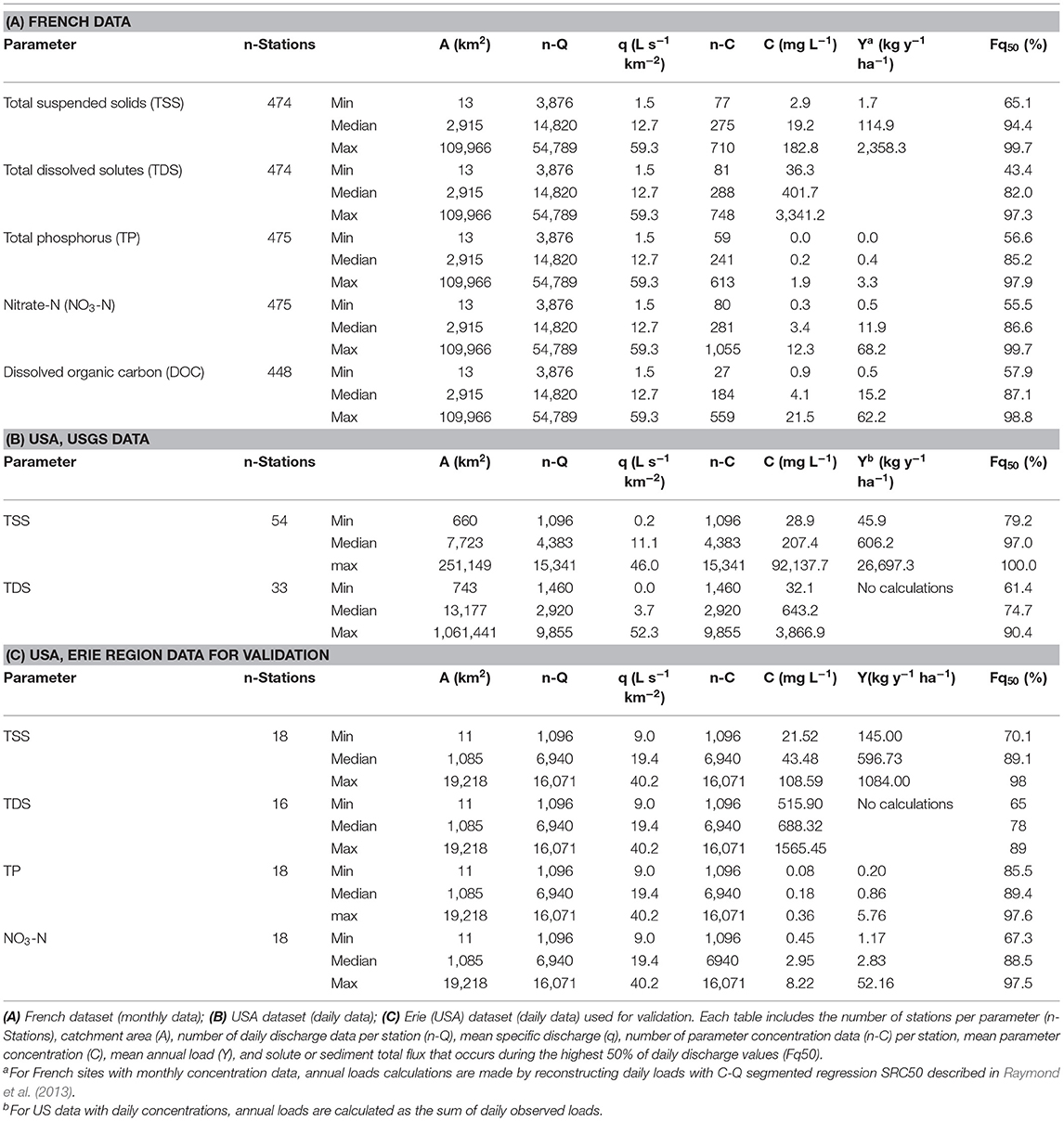
Table 1. Summary of datasets.
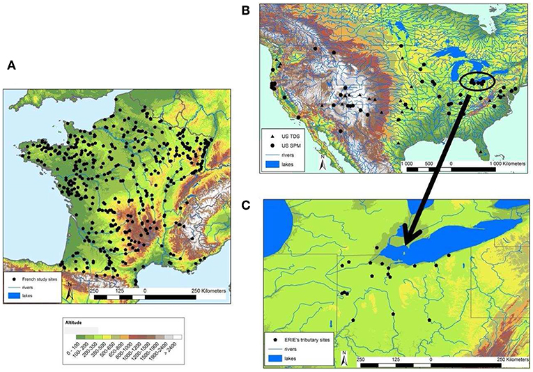
Figure 1. Sampling site locations for the following datasets: (A) France (monthly data), (B) USA (daily data), and (C) Erie (daily data).
We selected sites in the USA (Table 1B) that had at least 4 years of daily Q data; some sites had as much as 50 years of such data. We also gathered 4–50 years of data at sites with daily TSS and TDS data. These USA data were accessed via the USGS database (https://waterdata.usgs.gov/usa/nwis/). The selected USA catchments were in temperate or semi-arid ecoregions ranging from 650 to 250,000 km2. This dataset will from now on be referred as the USA database.
We also selected other USA data to serve as validation sites. The validation dataset encompassed 18 tributaries of Lake Erie (Table 1C) monitored by the National Center for Water Quality Research (NCWQR) at Heidelberg University in Ohio, USA. USGS provides the continuous Q data for these monitoring stations. Daily data on TSS, TDS, TP, and NO3-N, was collected for 4–50 years. Data was accessed at https://ncwqr.org/monitoring. These Erie catchments were under temperate or continental climatic conditions and range in area from 19 to 19,000 km2. This dataset will from now on be referred as Erie database.
Methods
Flow and Load Flashiness Indices
Definitions
Flow flashiness can be measured by the proportion of flow being discharged during the p% highest-flow days. This proportion is often much higher than p%, reflecting the fact that much of the flow is concentrated in a small proportion of time. It theoretically ranges between p%, for a river with constant discharge, to 100% when all the flow is passed in p% of time.
Formally, let F(x) denote the cumulative distribution function (cdf) of daily discharge. The flow flashiness index Wp is defined as follows:
F−1(1 − t) is the flow duration curve (i.e., the daily discharge exceeded with probability t). Wp can therefore be interpreted as the area below the flow duration curve up to p%, relative to the total area below the curve (Figure 2A).
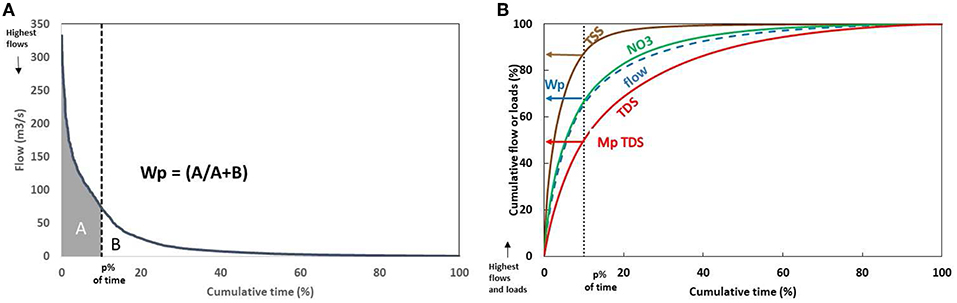
Figure 2. Illustration of flow and load flashiness indices for Portage River (1,109 km2), Ohio, USA. (A) The flow duration curve (FDC) characterizes the percentage of time a given flow is equaled or exceeded during a specified period. Wp is the area below the FDC up to p% (shaded gray), relative to the total area below the curve. (B) Plot of the cumulative percent of flow and constituent loads discharged during the p% highest-flow/load days. Wp is the value on y-axis for p% of time. Mp TSS, Mp TDS and Mp NO3 are percentages of loads of total suspended solids (TSS), total dissolved solutes (TDS), and nitrate (NO3) carried in the p% highest-flow days.
In practice Wp can be estimated from an observed series of daily discharge Q1, …, Qn. Let Q(1) ≥ … ≥ Q(n) denote the daily discharge sorted in decreasing order, and let k = ⌊n*p%⌋ denote the index corresponding to p% of the n days (⌊·⌋ is the integer part). Then:
Note that the flashiness index is not restricted to flow variables.
The load flashiness index Mp can be computed in the same way as Wp by simply replacing daily discharge (Q) with daily loads (L), calculated as below:
Equation (4) allows the calculation of Mp only when daily loads are available. Below, we estimate Mp when daily concentrations and loads are not available.
Differences between Mp and Wp are linked to the properties of the concentration-discharge (C-Q) relationship (Moatar et al., 2013). For perennial rivers, it is possible to mathematically demonstrate the expression of Mp as a function of Wp under the following assumptions (see Appendix for the complete details):
i) Daily flows follow a lognormal distribution, i.e., log(Q) ~ N(μ, σ)
ii) Daily concentration can be derived from daily flow using the C-Q regression:
The load flashiness for site i and constituent j, Mpi,j, can be written, under these assumptions, as a function of Wpi (flow flashiness for site i) and the parameters bi,j and ηi,j of the C-Q regression:
Where ϕ is the standard normal cdf and ϕ−1 its inverse (also known as the probit transformation):
Note that a “good” C-Q relationship would be characterized by a small residual standard deviation (ηi,j) compared with the standard deviation of input log-discharge (σi). In such a case, and the relation simplifies to:
Moatar and Meybeck (2007) and Moatar et al. (2013) tested different durations for p% of time (1, 2, 5, 10, 50%) over 125 stations in the USA and several constituents. They distinguished duration curves evaluated for each year and for the whole period of record. The proportion of the highest constituent loads (M1, M2…M50) and water volume (W1, W2, … W50) reached in 1, 2 … 50% of time are key indicators of river-borne material and flows patterns at a given station. They showed that for river TSS, the proportion of fluxes transported during a given percentage of time was always much higher than the proportion of river flow, and conversely, for TDS, this proportion was lower, as shown in Figure 2B. They chose the M2 indicator based on the analysis of statistical distribution of W1, W2, … W50, and M1, M2, … M50 for all water quality variables and stations. M2 was more accurately defined than M1. At durations of p > 5% in certain watersheds (e.g., smaller catchments and/or ephemeral streams with highly flashy and episodic load and flow regimes) the proportion of total annual loading of river-borne material was found to exceed 99%. Given our interest in creating a metric that could be applied across a range of river types and constituents, we set the flashiness index at p% = 2% (i.e., M2 and W2).
Empirical Approach for Estimating Load-Flashiness (M2) Depending on Flow-Flashiness (W2) and Export Pattern (b50high)
The formulation proposed in Equation (7) is similar to that proposed by Moatar et al. (2013) based on empirical adjustment, except that here we used a probit transformation for W2 and M2. However, our results showed that in many stations, especially for flashy rivers, daily discharge did not follow a lognormal distribution. The Equation (A1) (Appendix) for perennial rivers was tested for the French database. W2 estimated using this equation explained only 46% of the variance of observed W2 (calculated with Equation 2). Moreover, the dispersion of residuals increased with W2, i.e., for flashy rivers. Moreover, since log-linear analysis of the full extent of the C-Q relationship often did not adequately capture the variability of the data, Meybeck and Moatar (2012) and Moatar et al. (2017) proposed splitting C-Q curves at the median flow to separately analyze the C-Q relationships during low and high flows. They also demonstrated that, in all cases, the discharge above the median Q value transport between 70 and more than 99% of total load of dissolved and suspended matter. Thus, the exponent b50high (Equation 8) is a relevant control metric of dissolved and particulate material exports.
We name this b50high indicator as the “export pattern.” Negative b50high values reveal that the cdf of load increases less rapidly than that of river discharge (Figure 2B, see TDS curve for example) defining a dilution processes, either natural (e.g., salt springs) or anthropogenic (e.g., point-source pollution). Positive b50high values express an enrichment or mobilization process (e.g., TSS and TP). Therefore, we replaced “b” in the Equation (7) by “b50high.”
Equation (7), demonstrated mathematically, for p = 2% of time was tested for perennial rivers in the French database and five constituents replacing exponent “b” by “b50high.” We compared M2 estimates obtained with Equation (7) with reconstructed M2 (see below), for individual constituent and including the whole constituents together. We obtained very good estimates for solutes (R2 = 0.96) and TP (R2 = 0.90), but less for TSS (R2 = 0.67). When we account all constituents, R2 = 0.88.
Since our stations also include intermittent rivers, we decided to use an equation similar to Equation (7), calibrating the parameter α for all stations and constituents (French database and USA database) together (Equation 9). We tested the model by comparing the M2 predictions with observed M2 based on a set of independent daily loads for TSS, TDS, TP, and NO3 (Erie database).
for site i and constituent j, the calibrated α coefficient is 0.79.
This equation (Equation 9) explained 91% of M2 variance based on the French reconstructed daily loads using the C-Q relationship and the USA daily database with a root mean square error (RMSE) of 4% (Figure S1A). Moreover, for the Erie database (Figure S1B; not included in the calibration), 91% of variance of M2 is explained with W2 and b50high; the RMSE is 5%. Therefore, the combination of b50high and W2 constitutes a good proxy for M2 estimation when daily concentration data are not available.
M2 Reconstruction and Robustness From Discrete Concentrations Surveys and Daily Discharge
Reconstructed M2
To calibrate the parameter α on Equation (9), we used “true M2,” calculated from daily load available for USA database with Equation (4) and “reconstructed M2” calculated from monthly French database. Reconstructed M2 were determined after reconstruction of daily concentrations based on daily discharge using a segmented linear regression (Method SRC50 tested by Raymond et al., 2013) and Equations (8) and (10).
Q50 is the median discharge estimated from daily discharge. We tested statistical significance of C-Q correlation by Pearson product-moment correlation, with significant relationships (p < 0.05) depending on the slope. Most slopes were significant when b > 0.2 (Meybeck and Moatar, 2012), although the actual threshold varied depending on the number and variance of C-Q couples in the regression. We reported in Table S2, percentages of sites with significant correlations (p < 0.05) for segmented C-Q regressions.
To assess the robustness of M2 estimates derived from discrete surveys, we used two methods.
i) We validated the predictions of Equation (9) (M2 predicted) using the Erie database with “true M2” for four parameters and 18 rivers.
ii) We compared M2 estimates, obtained after the reconstruction of daily concentrations by segmented linear regression approach (Equations 8 and 10) with those obtained using the Weighted Regression on Time, Discharge, and Season approach (WRTDS; Q. Zhang pers. Comm.; Hirsch et al., 2010), a commonly used method (Lee et al., 2016; Zhang, 2018; Zhang et al., 2019). This was done on 248 French stations where monthly data of TSS, TP, and NO3, and daily Q where available for more than 40 years.
Analysis of b50high and M2 Variability Across Decades and Years
Equation (9) has been used with M2, W2, and b50high calculated from the entire set of data (between 20 and 40 years long). Since C-Q relationships can change with time, for example due to land use change, we assessed the stability of b50high and M2 across decades. To do so, we used the French dataset in four successive series of 10 years, i.e., 1978–1987; 1988–1997; 1998–2007; 2008–2017. Tukey's range test was used for the comparison of M2, b50high, and W2 across four decades and for the whole 40-y period to find means that are significantly different from each other. Additionally, we analyzed annual b50high variation for five stations in the Erie dataset where more than 35 years were available.
Minimal Length of Monitoring Required
We investigated the sensitivity of period length on estimated b50high and M2 considering monthly sampling (12 C-Q pairs per year). We used as reference the metrics computed from daily TSS, TDS, TP, and NO3, surveyed for more than 30 years in four rivers from the Lake Erie dataset with various watershed scales (386–15,395 km2). To mimic a classic long-term monthly monitoring, daily concentration time series were randomly subsampled following a normal distribution (30 days average ± 5 days). The metrics b50high and M2 were then computed on subsampled data and compared to reference values. To assess potential variations due to varying sampling dates, this was repeated 100 times for each given period length. We investigated this from 2 years-long timeseries, up to 20 years.
Determination of the Optimal Sampling Frequency
We used the formulations proposed by Moatar et al. (2013) to predict the magnitude of uncertainties (bias and precision) of loads and mean concentration using the discharge-weighted method. This method is commonly used by the Helsinki Commission (HELCOM) Baltic Sea Action Plan and by the Convention for the Protection of the Marine Environment of the North-East Atlantic (OSPAR), international European conventions on river pollutant loads to coastal zone (Littlewood and Marsh, 2005). The equations are:
where e10 and e90 = lower and upper limits of precision; d = sampling interval in days; r, s, u, v values for calculating precision for different d are available in Table S1. We used this formulation to derive an optimal sampling monitoring given an imposed ±10% as a level of precision (Figure 3). See Moatar et al. (2013) for more explanation on the method and formulations for biases.
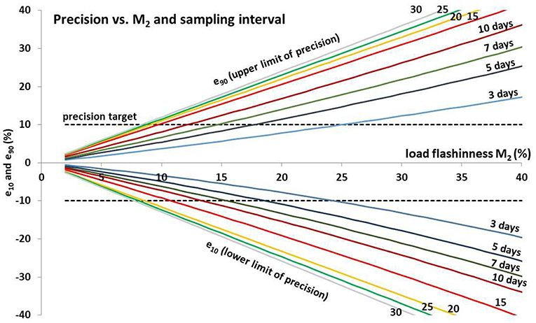
Figure 3. Error nomograph (e10, e90 vs. M2) for annual loads calculated for discharge-weighted concentration method (adapted from Moatar et al., 2013). Lower limits (e10) and upper limits (e90) for sampling intervals of 3, 7,…, 60 days. M2 is the percentage of cumulative load that occurs during the highest 2% of daily load values.
Relationship Between Catchment Characteristics and W2, b50high, and M2
We analyzed the main geographical, geological and land cover characteristics of 475 French drainage basins. We then determined relationships between these variables and W2, b50high, and M2 for each of the water quality parameters. We performed generalized additive model (GAM) to assess potential non-linearity in relationships. The results showed that smoothing functions poorly improved the regression models. Hence, we assumed that classical multivariate regressions would be convenient to highlight and discuss simple relationships including their sign.
We used multiple linear regressions to evaluate the relationship between French dataset characteristics, i.e., catchment size, agricultural land use, lithology, wetland surface, stream network density, erosion indicator risk, as well as W2, b50high, and M2 for each of the water quality parameters, i.e., TSS, TDS, TP, NO3, and DOC. These variables are listed with full details provided in Table 2. Starting with all explanatory variables in initial regression models, we used a backward selection approach to select only the significant ones (at p < 0.001). To assess the relative contribution of the selected variables, a hierarchical variation portioning was performed on each final model using the R package hier.part (Walsh and MacNally, 2013).
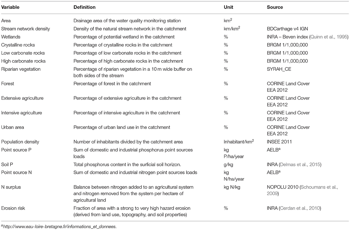
Table 2. List of explanatory variables and their definitions, units, and data sources.
Results
Flow-Flashiness (W2) and Export Pattern (b50high) Indicators
The interannual flow-flashiness indicator of the study sites (W2) ranged between 3 and 60%, with the majority between 5 and 30% (Figure 4). The high W2 values were obtained for USA semi-arid sites (W2 = 48% for San Pedro River, Arizona; 60% for Santa Clara River, California) and the French Mediterranean catchments (W2 = 39% for Agly River, Pyrénées Orientales). Low W2 values were found for groundwater-influenced streams (W2 = 3% for Ill River, France), glacial or nival regimes (W2 = 7% for Arve River and Romanche River, Alps, France), or by impoundments (W2 = 4% for Columbia River near Quincy, OR, USA or 6% for the Rhône River in France).
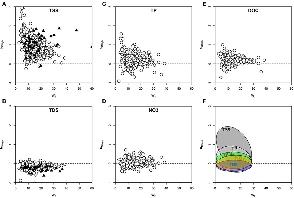
Figure 4. (A–E) Distribution of solutes and suspended solids in sampling sites along the W2 (proportion of flow discharged during the top 2% of days) and b50high (slope of the split C-Q relationship above median flow) relationship for total suspended solids (TSS), total dissolved solutes (TDS), total Phosphorus (TP), nitrate (NO3), and dissolved organic carbon (DOC) (White circles—French sites; black triangles—USA sites). (F) Envelops of parameters' variability along the W2 and b50high relationship. Ellipses represent 95% confidence clouds for each group of constituents.
The range of b50high varied depending on the water quality variables considered; but for a given variable, the range obtained from monthly sampling data (French dataset) did not significantly differ from the ones obtained from daily sampled data (USA dataset; Figures 4A,B). More specifically, TSS generally presented a positive chemodynamic pattern with b50high values > +0.2 and reaching up to 3 (Figure 4A). For the French dataset, high positive b50high values generally corresponded to streams with low flashiness, i.e., W2 < 15%. Some catchments in the Alps' mountains with snow hydrological regime (low W2) and influenced by hydroelectric dams were characterized by a very high export pattern (b50high between 2 and 3) due to yearly flushing dam management to maintain river-bed sediment dynamics and to prevent siltation (Nemery et al., 2013). Some coastal Californian stations (Eel and Santa Clara Rivers) and Colorado Plateau streams (San Pedro and Paria Rivers) presented both high W2 and b50high for TSS. On the contrary, TDS generally showed a negative chemodynamic pattern, i.e., dissolved ions are diluted when discharge increases (Figure 4B), regardless of the flow flashiness (W2).
TP, often transported with sediment, followed a similar pattern as TSS but with a smaller range of variation (Figure 4C). A positive export pattern (b50high) for TP was found for 84% of data with most export pattern values < 1. The b50high for TP was negative for 16% of data indicating dilution. Seventy percent of NO3-N presented a chemostatic pattern across all values of flow flashiness considered (Figure 4D). Nitrate mobilization in the drainage basins was proportional to discharge. DOC also presented a positive chemodynamic pattern for 50% of the studied catchments, but the high W2 sites were characterized by a more stable, chemostatic pattern (Figure 4E). Envelops of variability of the b50high-W2 relationship presented a rather distinctive shape, even though parameters overlapped (Figure 4F, ellipses represent 95% confidence clouds for each group of constituents).
The variability of annual W2 differed depending on climate and catchment hydrology. Differences between maximal and minimal annual W2 values ranged between 40 and 60% for catchments exposed to a contrasting climate (e.g., small catchments in the Mediterranean area experiencing hot and dry summers and intense short rainy events in autumn; catchments with no storage capacity resulting in severe low-flow and quick runoff response to rainfall events). Ranges <20% were observed for streams fed by large aquifers (e.g., northern France) or in catchments where snow pack storage buffers the variability of daily flows.
Variability of Load Flashiness (M2)
Interannual load-flashiness indicator values ranged between 2% (TDS for Ill River at Strasbourg) and 98% (TSS at Santa Clara River)—close to the possible range (2–100%) (Figure 5A). The distribution of M2 values was highly skewed, with 50% of values lower than 22%, and 75% lower than 27%. The range of M2 varied between solutes; M2 increased in the following order: TDS, NO3, DOC, TP, and TSS. Based on this statistical distribution of M2, we defined five classes. The upper boundary of the lowest class was 8% with each subsequent boundary representing a doubling of the prior upper limit. The median class contained the median statistical distribution value. The very low class of flashiness (M2 ranging between 2 and 8%) corresponded to negative or low b50high and low W2 (Table 3, Figures 5A,B). The low class of flashiness corresponded to M2 between 8 and 16%. The medium class of flashiness corresponded to M2 between 16 and 32%. The high class of flashiness corresponded to M2 between 32 and 64%. The very high class of flashiness (M2 > 64%) corresponded to strongly positive b50high and high W2. The proportion of the total number of studied stations in each class of load flashiness varied according to the constituents (Table 3). DOC, NO3, and TP generally were found in the low and medium load flashiness classes, while TSS was found in medium and high classes. TDS was more widely distributed between very low, low, and medium load flashiness classes. The relationship between M2 and W2 were similar on an annual and interannual basis (Figure 5). On both annual and interannual basis, M2 was generally higher than W2, i.e., points above the 1:1 line, for all the constituents (with positive b50high), except TDS which present mostly negative b50high.
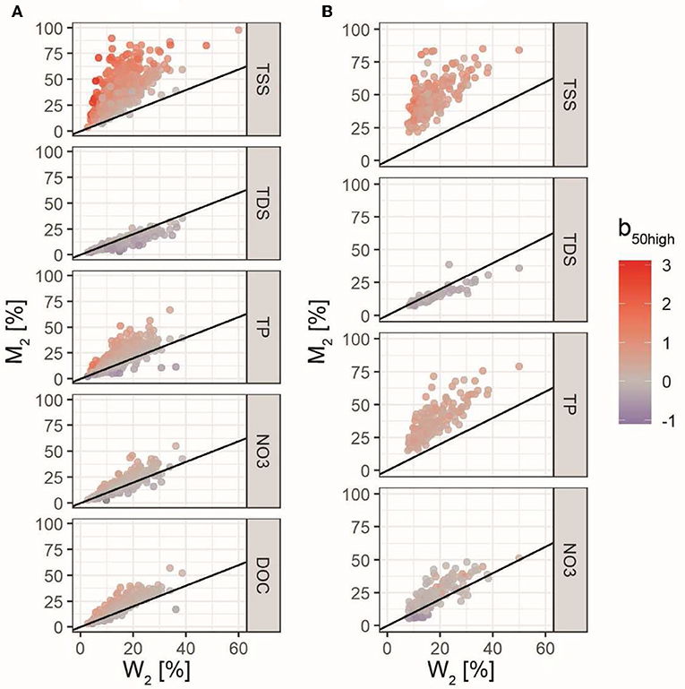
Figure 5. (A) Relationship between interannual M2 (load flashiness) and W2 (flow-flashiness) for monthly French dataset and daily USA dataset, computed for total suspended solids (TSS), total dissolved solids (TDS), total phosphorus (TP), nitrate (NO3), and dissolved organic carbon (DOC). (B) Relationship between annual M2 and W2 for daily Erie dataset, computed for total suspended solids (TSS), total dissolved solids (TDS), total phosphorus (TP), and nitrate (NO3). Dot color is a function of b50high (slope of the logC-logQ relationship for discharge higher than daily median discharge Q50 values); see color scale inserted in the right of the figure.
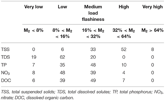
Table 3. Distribution of the 2,507 sample series (percentage) in each class of load flashiness depending on the solutes or particulates.
Using Equation (9), we drew M2 isolines representing the five classes' limits on the W2–b50high relationship (Figure 6A). The diagram permitted comparisons of M2 values between streams and/or presents the M2 differences between constituents for a given stream, as illustrated for four tributaries of the Lake Erie, USA with contrasting W2 (Figure 6B). The diagram of solute and export regime is presented in Figure 6C.
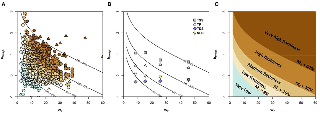
Figure 6. (A) Representation of the load flashiness M2 indicator (load flashiness) as a function of W2 (flow-flashiness) and b50high (export regime). Each color represents a class of flashiness. The color of the points corresponds to the class given by the observed M2. The lines are derived from Equation (9). (B) Examples of M2 values for four water quality parameters (TSS, TDS, TP, and NO3) of four Erie Lake tributaries of increasing areas. The color of the points corresponds to the class given by the observed M2. The lines are derived from Equation (9). (C) Diagram of load flashiness and five classes of flashiness from very low flashiness with M2 < 8%, to very high flashiness with M2 > 64%.
M2 and b50high Robustness
Influence of the Concentration Reconstruction Method to Estimate M2
The two methods used to reconstruct daily concentrations led to similar results. The standard deviation of differences in the estimates of M2 calculated with daily concentrations reconstructed with the WRTDS and the segmented C-Q method (M2WRTDS-M2SRQ50) was around 4% for NO3 and TP for the four decades considered and 12% for TSS (Data presented in Figure S2). The mean difference of M2 estimates was zero for NO3, but it was +4% for TSS and +2% for TP. For these two last parameters, M2 estimated by WRTDS method were larger than estimates for the C-Q segmented method (Figure S2).
Analysis of b50high and M2 Variability Across Decades and Years
For the French dataset, where we have up to 40 years of data, b50high for TSS, TDS, NO3, and DOC showed little variation across decades, while we found some noticeable, but not significant differences for TP. Overall, the variability between the four decades was limited for TSS (<5% for median M2 and <0.05 for median b50high), TDS, DOC and nitrate (<1% for M2). For TP, b50high was higher in the last period (2008–2017) (+0.2) than in first and second periods (1978–1987 and 1988–1997). This was due to a more pronounced dilution of punctual sources which were more important in the 1978–1997. Therefore, the load-flashiness was lower (−5%) in the first period compared to the present time. However, the differences were limited.
For yearly variations in the Erie dataset, differences were more important across years, which was particularly true for Cuyahoga and mostly for TSS, TDS, and TP (Figures S3, S4). For the other studied rivers, the variations of annual b50high were more limited, even if some years could have a more pronounced export pattern (b50high).
Minimal Length of Monitoring Required for Determining b50high and M2
Sensitivity of period length necessary to derive reliable b50high and M2 estimates from monthly monitoring was assessed via subsampling of daily timeseries (Figure 7). Results showed site-specific and metric-specific sensitivities but overall differences between monthly-based (median after 100 random draws) and daily-based values were systematically decreasing with longer period length. Relative bias was smaller for b50high and higher for M2, in particular for TSS at Honey Creek station which was the only timeseries presenting large bias (−62% bias even for timeseries longer than 10 years). Variability across the 100 random draws was reduced for both metrics computed from longer timeseries and for all constituents despite larger variability for b50high computed for NO3 data (±60%). Results indicated that 10 years-long monthly timeseries represented a reasonable amount of observations for coherent estimation of these two key metrics.
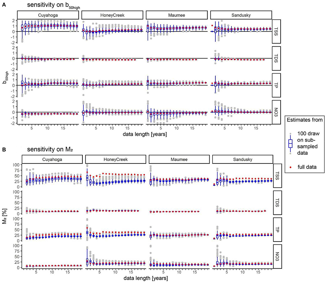
Figure 7. (A) Sensitivity analysis of b50high and (B) of M2 estimates for various time lengths and two sampling strategies: metrics derived from daily data are represented with red dots; metrics derived from 100 monthly subsamples random draws for each time length are represented with blue boxplots.
Implications for Sampling Frequency
The optimal sampling frequency needed to minimize the uncertainty associated with the estimation of solute and sediment loads increased with increasing M2 (Figure 8). Based on Equations (11) and (12), we obtained that for M2 of 8% or less, a monthly sampling would be sufficient to obtain load estimation with 10% of precision. If M2 was 16%, a weekly sampling would be required to keep the same level of precision. If M2 was more than 32%, a sub daily sampling would be necessary.
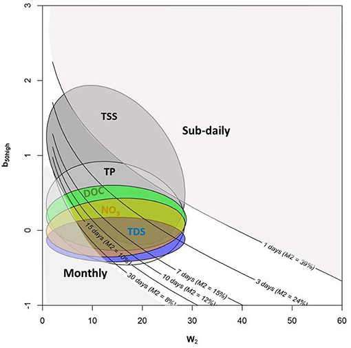
Figure 8. Sampling intervals required to achieve targeted errors (precision ± 10%) on annual loads as a function of b50high and W2. Each sampling interval corresponds to a level of load flashiness (M2) calculated by error nomograph parameters (adapted from Moatar et al., 2013). Ellipses represent 95% confidence clouds for each group of constituents. For M2 > 40%, high frequency monitoring, i.e., 3 days or 1 day, would be necessary. For M2 < 8%, monthly monitoring is sufficient to achieve a ± 10% precision.
The comparison of the optimal frequencies to calculate annual loads with <10% precision using our approach and the current sampling frequency recommended by the European Water Framework Directive is presented in Figure 9. This revealed that more than 90% of the existing monitoring strategies would fail to accurately calculate annual loads of solutes and particulates transported by French streams and rivers with the Q-weighted concentration method, a method commonly used by HELCOM and OSPAR international European conventions on river pollutant loads to coastal zone. The load-flashiness diagram informed that each catchment and constituent needs specific monitoring strategies to obtain load estimates with good precision. TDS needs lower sampling frequencies than NO3 and DOC. Also, constituents associated with suspended sediments, like TP, need more frequent sampling. TSS required high frequency for the majority of stations. The median of optimal sampling interval between two measurements required for the French dataset was: 13 days for TDS, 8 days for NO3, 6 days for DOC, 5 days for TP, and every day sampling for TSS.
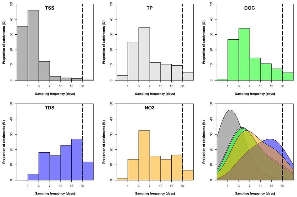
Figure 9. Distribution of optimal sampling intervals required for 475 French stations for each parameter. The vertical dashed lines represent the current sampling frequency, i.e., monthly, used by national monitoring survey based on European Water Framework Directive.
Influence of Catchment Characteristics on Nutrient, Carbon, and Sediment Export Regimes
Catchment characteristics explained up to 38% of the total variance of W2, b50high, and M2 (Table 4; first line). Individual contributions (between 0 and 100%) of the selected variables (see Table 2) according to hierarchical variation partitioning are indicated below. In Table 4, blue and red cells indicate positive and negative relationships, respectively.
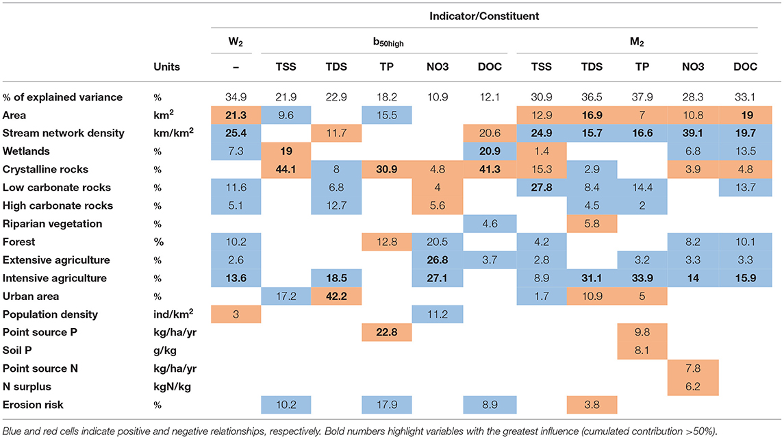
Table 4. Relationships between W2, b50high, and M2 indicators and catchment characteristics: total percentage of variance explained by final regression models following a backward selection approach of explanatory variables (third column) and individual contributions (between 0 and 100%; next columns) of the selected variables according to hierarchical variation partitioning.
W2 was positively related to the stream network density and the percentage of intensive agriculture in the catchment (25 and 13% respectively) while it decreased with the size of the drainage basin (21%). The b50high values of TSS, TP and DOC (between 31 and 44% of variance explained) decreased with the percentage of crystalline rocks in the catchments. We found a significant positive relationship between the percentage of wetland in the catchment and the DOC b50high (21%), while a negative relationship was found for TSS b50high (19%). The percentage of intensive agriculture in the catchment had a significant positive influence on TDS b50high (18%). Load flashiness (M2) decreased with the size of the catchment for all the water quality parameters, while it increased also for all the water quality parameters with the stream network density and the percentage of intensive agricultural practices.
Discussion
Load Flashiness (M2) Evaluation With Flow Flashiness (W2) and Export Pattern (b50high)
We found that load flashiness (M2) can be inferred from flow flashiness (W2) and export pattern (b50high) based on a large dataset of stream concentration and discharge encompassing a wide range of climatic, geologic and land use conditions. We characterized the flashiness of solute and sediment export regime (M2) using hydrological and biogeochemical indicators calculated for high flows, i.e., the flow flashiness (W2) and the exponent of C-Q relationships during discharge higher than the median (b50high). Following previous studies, we determined that stream export of solute and sediment during the highest 2% of time (M2) was a good indicator of solute and sediment transport. We proposed to overcome the lack of high frequency concentration measurements by using the exponent of C-Q relationships during high flow periods (b50high) as a proxy for export pattern, coupled with flow flashiness—a parameter more easily available, thanks to continuous discharge monitoring or new modeling development for ungauged catchments (Oudin et al., 2008).
The theoretical proposed approach is based on two assumptions which have some implicit limitations. The first assumption (see Appendix for detailed demonstration) is that the distribution of daily Q is lognormal with parameters μ (mean of logarithms) and σ (standard deviation of logarithms). However, daily flow might not be lognormal. For instance, in intermittent streams, a specific term may be needed to describe the occurrence of zero flows. Moreover, the distribution of daily flows may be heavy-tailed leading to more extreme flows than suggested by the lognormal distribution. Therefore, flow variability might be described by other metrics in addition to σ, such as the probability of zero flows or some tail coefficient. The second assumption is that the daily concentration C can be derived as a power function of the daily flow, C = aQb. This implies that the daily load is equal to:
L = CQ = aQb+1 which is a raw approximation. In particular, C-Q data typically show a large scatter around this power relationship. This scatter creates an additional source of variability that might play a non-negligible role on the variability of loads, and hence on the flashiness M2. The regression formula of Equation (7) could therefore be augmented with an additional predictor describing the variability of the residuals around the C-Q power relationship.
Despite these assumptions, the theoretical model for perennial rivers (Equation 7), and the empirical model (Equation 9) provide good predictions of load flashiness (M2). The empirical model (Equation 9) was parameterized based on an extensive monthly-sample data set from France (TSS, TDS, TP, NO3, and DOC) and daily-sample data set from USA (TSS and TDS). The model was validated using an extensive daily-sample dataset (TSS, TDS, TP, and NO3) from several rivers near Lake Erie. However, a more diverse validation dataset would have been desirable. Yet, daily concentrations with long-term time series are very rare.
M2 can be calculated by different methods depending on sampling frequency of concentration. When high-frequency concentration data are available, daily loads can be derived and Equation (4) can be applied. When discrete surveys are available, for example monthly samples, there are two options to characterize the M2. One can apply Equation (4) after reconstruction of daily concentrations with a regression method like WRTDS (Hirsch et al., 2010) and LogC-LogQ regression (Raymond et al., 2013; Moatar et al., 2017; Minaudo et al., 2019). Or it is possible to apply theoretical (Equation 7) (for perennial rivers) or empirical (Equation 9), both depending on W2 and export pattern (b50high). W2 can be easily determined, and b50high can be predicted depending on constituent. For example, the diagram of load-flashiness (Figure 6C) can give indicative values of classes of flashiness depending on these two indicators. The choice of 2% duration to define flow and load flashiness was suggested here to be representative of duration for many constituents. If studies focus on specific constituents, the question of choice of duration could be evaluated. For example, Frazar et al. (2019) analyzed durations of 2, 5, and 10% to characterize contrasting behavior of nitrate and phosphate loads from high flow events on small catchments. Moreover, this approach allows the decoupling of flow flashiness and export pattern to discern distinct patterns which could be related to drainage basin characteristics, climate change or land use change (Table 4, discussed below).
Characterization of Solute and Sediment Export Regimes Across Various Range of Catchments
Our databases cover a wide range of climatic, lithological, land use and hydrological conditions found in the northern hemisphere between 30° and 50°N and range across river magnitudes from 10 km2 to 1 million km2. The database displays extensive ranges of concentration and river flow which are close to those observed at the global scale for river basins of similar sizes (Meybeck and Helmer, 1989; Meybeck et al., 2003). We argue that the ranges of the indicators obtained here are also close to their global distributions in these latitudes, and thus our results can provide guidance in many settings.
C-Q relationships are important signatures of catchment biogeochemical processes and export regime (Moatar et al., 2017). Separately analyzing the C-Q relationships during low and high flows improves estimates of non-linearity and potential shift effects in hydrological and biogeochemical controls under different hydrological regimes (Underwood et al., 2017; Diamond and Cohen, 2018). The range of export pattern, b50high, is more contrasted than b calculated from the whole hydrograph, as conducted by Godsey et al. (2019) in a similar large database.
The relationship between discharge and concentration has significant implications for the inequality of solute export dynamics. Indeed, differences between cumulated percentage of load and flow associated with a specific duration or the ratios of Gini coefficients depend on the C-Q relationship (Jawitz and Mitchell, 2011; Moatar et al., 2013). If the C-Q relationship is chemostatic (b = 0, constant C), discharge and load have the same Gini Coefficients (GL/GQ = 1). When C-Q relationship is negative (b < 0), often indicating a dilution signal, the inequality of load is smaller than discharge (GL/GQ < 1). When C-Q relationship are positive (b > 0) revealing an enrichment signal, the inequality of load is greater than the discharge's one (GL/GQ > 1).
Our framework for estimating load flashiness can be compared to the bivariate plot of beta and the coefficient of variations ratio proposed by Musolff et al. (2015), based on the ratio of coefficient of variation of the concentration to discharge. Our load-flashiness diagram (Figure 6C) is based on b50high–shown to be more selective in characterizing the export regimes between constituents (Underwood et al., 2017)—and presents a large dataset (over 1.5 million measurements). As a result, our load-flashiness diagram (Figure 6C) presents a larger dispersion, especially for chemodynamics export regimes. Moreover, proposing to replace the Musolff et al. (2015) export regime with W2, a proxy more directly related to variation of discharge, will help determine the impact of hydrological change, such as those potentially induced by climate change on load exports. Flow flashiness (W2) is a proxy of hydrological reactivity, which includes surficial and groundwater inputs. Deciphering between these different water sources could be assessed by examining patterns of their specific solute tracers as proposed by Li et al. (2017) and Zhi et al. (2019).
Optimizing Sampling Frequency for Reducing Load Calculation Uncertainty
Our results provide a water quality monitoring strategy that can address the large range of M2 values measured in our dataset for different solutes and catchments (Figure 8). We demonstrated that relationship between uncertainties and loads flashiness M2 combined with b50high, can be used to calculate bias and precision for a given sampling frequency. Because sampling interval curves correspond to different M2 values (e.g., Figures 8, 9 displayed results for a targeted uncertainty of 10%), these results can also be used to determine the optimal sampling frequency for a given uncertainty (Moatar et al., 2013). Uncertainties of the different load estimates may vary substantially, depending on the particular solute and particulate, differences in hydro-climate, and basin size. The method considers both the river-borne constituent considered and the hydrological characteristics of the catchments. Hence, sampling frequency should be adapted to each station and each solute or particulate, characterized by W2 and b50high, if a given regulatory uncertainty level is required. For instance, to characterize and manage eutrophication risks related to total phosphorus inputs from smaller catchments (medium flashiness class, chemodynamic behavior) to freshwater lakes requires more intensive sampling than nitrate inputs from larger catchments (low flashiness class, chemostatic behavior) that can stimulate coastal zone eutrophication. Yet, an adaptive sampling strategy is rarely achieved in existing surveys. In France, the national monitoring program, designed to fulfill the European Water Framework Directive, recommends a fixed monthly sampling frequency, whatever the water-borne material or the catchment size considered. Yet, our results (Figure 9) show that a 30 days sampling frequency is not appropriate to calculate loads with a reasonable uncertainty (±10%) in more than 90% of cases. Our approach to determine M2, based on W2 and b50high, allows the determination of optimal sampling frequency, but also provides a measure of imprecision of past load measurements based on inadequate frequencies. Therefore, past load trends for the last 20–30 years can be recalculated, even based on classical monthly frequency. Based on these load trend recalculation, one can, for example, evaluate response-time of drainage basins to a given land use change and/or water policy implementation. Moreover, effects of potential hydrological changes (resulting in different W2) based on climate change scenarios on loads, could be estimated with more accuracy.
Drainage Basin Characteristics as Predictor of M2, b50high, and W2
Our study is the first to our knowledge that analyses the environmental factors controlling load variability (M2). Although, the total explained variance is relatively low, i.e., 28–38% depending on the constituent (Table 4), one should emphasize that it represents the variance explained by an indicator of load variability. Indeed, trying to explain the variance of a variability is not an easy task, especially because our approach does not consider the temporal successions of climatic and hydrological events. Explained variance could likely be improved with other proxies, such topographic and hydroclimatic indicators. However, a still significant part of the variance of the studied solute flashiness (M2) and its proxies, i.e., W2 and b50high, could be explained with a multi-variate model of widely-available drainage basin characteristics, e.g., drainage basin size, percentage of intensive agriculture and percentage of stream network density (Table 2). Many studies since the 1970s have attempted to relate inter-annual means of solute concentrations and loads with drainage basin lithology, land cover and land use (Dupas et al., 2015). For instance, Omernik (1976) found a significant relationship between percentage of cropland in the drainage basin and nitrogen and phosphorus loads. Jones et al. (1976) reported a significant negative relationship between the percentage of wetlands in the drainage basin and nitrate loads—the very first large scale hint of the role of denitrification in wetland as a mechanism to buffer nitrate loads. In a large-scale study, Aitkenhead and McDowell (2000) calculated that mean soil C/N ratio of a biome accounted for 99.2% of the variance in annual riverine DOC concentrations. Yet, these large-scale relationships do not hold when analyzing smaller drainage basins, i.e., <few hundreds of km2 often corresponding to the local water management scale, due to major influence of the spatial arrangements of land uses and the heterogeneity of geology and topography in solutes loads (Burt and Pinay, 2005; Abbott et al., 2018). Hence, the significant negative relationship between M2 and drainage basin size, which stresses the need to focus more intensive monitoring on small catchments if we want to quantify catchment flashiness. Indeed, in small catchments lateral inputs of nutrients and carbon during high water period are often orders of magnitude higher than instream retention or removal (Brookshire et al., 2009). The significant positive relationship between percentage of intensive agriculture and both load and flow flashiness (M2 and W2) agrees with the idea that a similar positive significant relationship occurs with water flashiness (W2). Intensive agriculture practices often simplify the landscape, creating open fields, removing hedgerows, rectifying streams and draining soils (also positively related to flashiness, Table 2). All these practices contribute to increased runoff and to the reduction of solutes and particles retention. Hence, since a higher degree of water and transported constituents' flashiness is expected in intensive agriculture catchments, they require a more frequent monitoring design.
Differences in load flashiness among the various waterborne materials align with catchment variations in the sources and fate of those materials. For example, the positive relationship between DOC flashiness and the percentage of wetlands confirms their significant contribution to stream DOC (Zarnetske et al., 2018). The negative relationships between percentage of crystalline rocks or schist parent material on TSS, TP, and DOC export pattern, reveals a generally less intensive agricultural activity on these parent materials. This pattern may also be due to a dilution of these constituents by deep groundwater during high flow events (Thomas et al., 2016). It is worth noticing that nitrate exhibited a biogeochemical stationary behavior (sensu Basu et al., 2010), with b50high mostly close to zero values. This result suggests a legacy storage of antecedent intensive fertilization (Aquilina et al., 2012; Van Meter et al., 2016), However, b50high was significantly positively relate to the percentage of agriculture, which implies that during high water regime, nitrate stock mobilization in agricultural catchments can still increase with discharge increase. This finding underlines the necessity to tailor monitoring schemes to catchment characteristics. Although many nitrate monitoring schemes may warrant lower intensity in many situations, sampling intervals in agricultural catchments should be shortened, especially in the context of more frequent intense rainfall events under climate change.
Conclusion
We were able to demonstrate that load flashiness (M2), i.e., percentage of cumulative load that occurs during the highest 2% of daily load values is a useful proxy of solute and sediment export regimes. Our results emerged from a robust, long-term dataset of a wide range of discharge, solute and particulate sediments in 580 drainage basins in France and the USA and 2,507 sample series, representing over 1.5 million discharge-concentration couples. This indicator can be estimated from the common low-frequency national or regional monitoring surveys through the b50high coefficient and the runoff flashiness indicator (W2). We showed that if current water-sampling strategies undertaken by local, national, and international water authorities are not appropriate to directly calculate solutes and sediment loads; these data can nevertheless be used to calculate flow flashiness (W2) and b50high. We demonstrated that these two proxies are related to load flashiness (M2) with a simple equation. We showed that load flashiness diagrams can be used to classify constituents and catchments by precision related to different sampling intervals and thus optimize stream water quality sampling procedures for a given transported constituent. Moreover, the analysis of our large dataset allowed the identification of significant correlations between easily accessible drainage basin characteristics (e.g., basin area, stream network density, and percentage of extensive agriculture), W2, b50high, and M2. These characteristics can serve as a basis to classify non-monitored drainage basins as a function of their potential load flashiness and propose a sampling monitoring design for the most contributive ones. Regulatory monitoring in Europe, recommended by the WFD, promotes the monthly sampling for any monitored constituents (dissolved and particulate) and for any basin size. Such standardized monitoring does not take into account the actual variability of the constituent concentration and loads, particularly for the small (100–1,000 km2) and very small (<100 km2) basins. The load flashiness M2 can also be used to optimize monitoring frequency to reach a certain level of annual load uncertainty (here 10%) for loads trend detection required for instance by international conventions such as OSPAR and HELCOM.
Data Availability Statement
The datasets generated for this study are available on request to the corresponding author.
Author Contributions
FM, GP, MM, BR, and AG wrote the first draft. FM, MFl, CM, and MFe analyzed the data and made the figures. AC made the spatial calculations. The final manuscript was written by FM, GP, BR, AG, and KA with contributions from all co-authors.
Funding
This work was funded by the French National Agency for Biodiversity (AFB). The authors are grateful to the French Water Basin Agencies and their partners who contributed to the water quality data acquisition.
Conflict of Interest
The authors declare that the research was conducted in the absence of any commercial or financial relationships that could be construed as a potential conflict of interest.
Acknowledgments
We would like to thank Qian Zhang (University of Maryland Center for Environmental Science) for the calculations of daily loads on 238 French stations with WRTDS method. We also would like to thank two reviewers for their very thorough and constructive comments on an earlier version of the manuscript. Their insights helped us to improve this current version.
Supplementary Material
The Supplementary Material for this article can be found online at: https://www.frontiersin.org/articles/10.3389/fevo.2019.00516/full#supplementary-material
Figure S1. Predicted M2 vs. observed M2. (A) For French sites (TSS, TDS, TP, NO3, DOC) and US (TSS and TDS) calibration set of data. (B) For streams of Lake Erie Region, data not used in the calibration procedure (TSS, TDS, TP, NO3).
Figure S2. Comparison analysis on 248 French stations of M2 estimates derived from segmented linear regression approach (Method SRC50) on monthly TSS, TP, and NO3, and daily discharge vs. M2 estimates derived from a Weighted Regression on Time Discharge and Seasonality (Method WRTDS, Q. Zhang pers. comm.).
Figure S3. Temporal evolution of yearly b50high estimated for TSS, TDS, TP, and NO3 on five long-term and daily Lake Erie tributaries datasets.
Figure S4. Temporal evolution of yearly M2 and W2 estimated for TSS, TDS, TP, and NO3 on five long-term and daily Lake Erie tributaries datasets.
Table S1. Error nomograph (e10, e90 vs. M2) for annual loads calculated for discharge-weighted concentration method. Lower limits (e10) and upper limits (e90) for sampling intervals of 3, 7,…, 60 days (Moatar et al., 2013).
Table S2. Percentage of sites with significant p-values for segmented C-Q regressions. Total suspended solids (TSS), total dissolved solutes (TDS), total phosphorus (TP), nitrate (NO3), dissolve organic carbon (DOC).
Abbreviations
W2, percentage of cumulative discharge that occurs during the highest 2% of daily discharge values, termed as flow flashiness; M2, percentage of cumulative load that occurs during the highest 2% of daily load values, termed as load flashiness; b50high, slope of the logC-logQ relationship for discharge higher than daily median discharge Q50, termed export pattern; C-Q, concentration-discharge; Q, discharge; Cdf, cumulative distribution function.
References
Abbott, B. W., Gruau, G., Zarnetske, J. P., Moatar, F., Barbe, L., Thomas, Z., et al. (2018). Unexpected spatial stability of water chemistry in headwater stream networks. Ecol. Lett. 21, 296–308. doi: 10.1111/ele.12897
Aitkenhead, J., and McDowell, W. H. (2000). Soil C: N ratio as a predictor of annual riverine DOC flux at local and global scales. Glob. Biogeochem. Cycles 14, 127–138. doi: 10.1029/1999GB900083
Aquilina, L., Vergnaud-Ayraud, V., Labasque, T., Bour, O., Molénat, J., Ruiz, L., et al. (2012). Nitrate dynamics in agricultural catchments deduced from groundwater dating and long-term nitrate monitoring in surface-and groundwaters. Sci. Tot. Environ. 435, 167–178. doi: 10.1016/j.scitotenv.2012.06.028
Basu, N. B., Destouni, G., Jawitz, J. W., Thompson, S. E., Loukinova, N. V., Darracq, A., et al. (2010). Nutrient loads exported from managed catchments reveal emergent biogeochemical stationarity. Geophys. Res. Lett. 37:L23404. doi: 10.1029/2010GL045168
Breitburg, D., Levin, L. A., Oschlies, A., Grégoire, M., Chavez, F. P., Conley, D. J., et al. (2018). Declining oxygen in the global ocean and coastal waters. Science 359:eaam7240. doi: 10.1126/science.aam7240
Brookshire, E., Valett, H., and Gerber, S. (2009). Maintenance of terrestrial nutrient loss signatures during in-stream transport. Ecology 90, 293–299. doi: 10.1890/08-0949.1
Burt, T., and Pinay, G. (2005). Linking hydrology and biogeochemistry in complex landscapes. Prog. Phys. Geogr. 29, 297–316. doi: 10.1191/0309133305pp450ra
Cerdan, O., Govers, G., Le Bissonnais, Y., Van Oost, K., Poesen, J., Saby, N., et al. (2010). Rates and spatial variations of soil erosion in Europe: a study based on erosion plot data. Geomorphology 122, 167–177. doi: 10.1016/j.geomorph.2010.06.011
Crowder, D., Demissie, M., and Markus, M. (2007). The accuracy of sediment loads when log-transformation produces nonlinear sediment load–discharge relationships. J. Hydrol. 336, 250–268. doi: 10.1016/j.jhydrol.2006.12.024
Delmas, M., Saby, N., Arrouays, D., Dupas, R., Lemercier, B., Pellerin, S., et al. (2015). Explaining and mapping total phosphorus content in French topsoils. Soil Use Manage. 31, 259–269. doi: 10.1111/sum.12192
Diamond, J. S., and Cohen, M. J. (2018). Complex patterns of catchment solute–discharge relationships for coastal plain rivers. Hydrol. Process. 32, 388–401. doi: 10.1002/hyp.11424
Dupas, R., Delmas, M., Dorioz, J. M., Garnier, J., Moatar, F., and Gascuel-Odoux, C. (2015). Assessing the impact of agricultural pressures on N and P loads and eutrophication risk. Ecol. Indic. 48, 396–407. doi: 10.1016/j.ecolind.2014.08.007
Ferguson, R. (1986). River loads underestimated by rating curves. Water Resour. Res. 22, 74–76. doi: 10.1029/WR022i001p00074
Frazar, S., Gold, A. J., Addy, K., Moatar, F., Birgand, F., Schroth, A. W., et al. (2019). Contrasting behavior of nitrate and phosphate flux from high flow events on small agricultural and urban watersheds. Biogeochemistry 145, 141–160. doi: 10.1007/s10533-019-00596-z
Gaillardet, J., Dupré, B., Louvat, P., and Allegre, C. (1999). Global silicate weathering and CO2 consumption rates deduced from the chemistry of large rivers. Chem. Geol. 159, 3–30. doi: 10.1016/S0009-2541(99)00031-5
Gall, H. E., Park, J., Harman, C. J., Jawitz, J. W., and Rao, P. S. C. (2013). Landscape filtering of hydrologic and biogeochemical responses in managed catchments. Landsc. Ecol. 28, 651–664. doi: 10.1007/s10980-012-9829-x
Godsey, S. E., Hartmann, J., and Kirchner, J. W. (2019). Catchment chemostasis revisited: water quality responds differently to variations in weather and climate. Hydrol. Process. 33, 3056–3069. doi: 10.1002/hyp.13554
Godsey, S. E., Kirchner, J. W., and Clow, D. W. (2009). Concentration–discharge relationships reflect chemostatic characteristics of US catchments. Hydrol. Process. 23, 1844–1864. doi: 10.1002/hyp.7315
Hirsch, R. M., Moyer, D. L., and Archfield, S. A. (2010). Weighted regressions on time, discharge, and season (WRTDS), with an application to Chesapeake Bay river inputs 1. J. Am. Water Resour. Assoc. 46, 857–880. doi: 10.1111/j.1752-1688.2010.00482.x
Jarvie, H. P., Smith, D. R., Norton, L. R., Edwards, F. K., Bowes, M. J., King, S. M., et al. (2018). Phosphorus and nitrogen limitation and impairment of headwater streams relative to rivers in Great Britain: a national perspective on eutrophication. Sci. Tot. Environ. 621, 849–862. doi: 10.1016/j.scitotenv.2017.11.128
Jawitz, J. W., and Mitchell, J. (2011). Temporal inequality in catchment discharge and solute export. Water Resour. Res. 47:W00J14. doi: 10.1029/2010WR010197
Johnes, P. J. (2007). Uncertainties in annual riverine phosphorus load estimation: impact of load estimation methodology, sampling frequency, baseflow index and catchment population density. J. Hydrol. 332, 241–258. doi: 10.1016/j.jhydrol.2006.07.006
Jones, J., Borofka, B., and Bachmann, R. (1976). Factors affecting nutrient loads in some Iowa streams. Water Res. 10, 117–122. doi: 10.1016/0043-1354(76)90109-3
Le Moal, M., Gascuel-Odoux, C., Ménesguen, A., Souchon, Y., Étrillard, C., Levain, A., et al. (2019). Eutrophication: a new wine in an old bottle? Sci. Tot. Environ. 651, 1–11. doi: 10.1016/j.scitotenv.2018.09.139
Lee, C. J., Hirsch, R. M., Schwarz, G. E., Holtschlag, D. J., Preston, S. D., Crawford, C. G., et al. (2016). An evaluation of methods for estimating decadal stream loads. J. Hydrol. 542, 185–203. doi: 10.1016/j.jhydrol.2016.08.059
Li, L., Bao, C., Sullivan, P. L., Brantley, S., Shi, Y., and Duffy, C. (2017). Understanding watershed hydrogeochemistry: 2. Synchronized hydrological and geochemical processes drive stream chemostatic behavior. Water Resour. Res. 53, 2346–2367. doi: 10.1002/2016WR018935
Littlewood, I. G., and Marsh, T. J. (2005). Annual freshwater river mass loads from Great Britain, 1975-1994: estimation algorithm, database and monitoring network issues. J. Hydrol. 304, 221–237. doi: 10.1016/j.jhydrol.2004.07.031
Meybeck, M. (1987). Global chemical weathering of surficial rocks estimated from river dissolved loads. Am. J. Sci. 287, 401–428. doi: 10.2475/ajs.287.5.401
Meybeck, M., and Helmer, R. (1989). The quality of rivers: from pristine stage to global pollution. Palaeogeogr. Palaeoclimatol. Palaeoecol. 75, 283–309. doi: 10.1016/0031-0182(89)90191-0
Meybeck, M., Laroche, L., Dürr, H., and Syvitski, J. (2003). Global variability of daily total suspended solids and their fluxes in rivers. Glob. Planet. Change 39, 65–93. doi: 10.1016/S0921-8181(03)00018-3
Meybeck, M., and Moatar, F. (2012). Daily variability of river concentrations and fluxes: indicators based on the segmentation of the rating curve. Hydrol. Process. 26, 1188–1207. doi: 10.1002/hyp.8211
Minaudo, C., Dupas, R., Gascuel-Odoux, C., Fovet, O., Mellander, P. E., Jordan, P., et al. (2017). Nonlinear empirical modeling to estimate phosphorus exports using continuous records of turbidity and discharge. Water Resour. Res. 53, 7590–7606. doi: 10.1002/2017WR020590
Minaudo, C., Dupas, R., Gascuel-Odoux, C., Roubeix, V., Danis, P.-A., and Moatar, F. (2019). Seasonal and event-based concentration-discharge relationships to identify catchment controls on nutrient export regimes. Adv. Water Resour. 131:103379. doi: 10.1016/j.advwatres.2019.103379
Moatar, F., Abbott, B. W., Minaudo, C., Curie, F., and Pinay, G. (2017). Elemental properties, hydrology, and biology interact to shape concentration-discharge curves for carbon, nutrients, sediment, and major ions. Water Resour. Res. 53, 1270–1287. doi: 10.1002/2016WR019635
Moatar, F., and Meybeck, M. (2005). Compared performances of different algorithms for estimating annual nutrient loads discharged by the eutrophic River Loire. Hydrol. Process. 19, 429–444. doi: 10.1002/hyp.5541
Moatar, F., and Meybeck, M. (2007). Riverine fluxes of pollutants: towards predictions of uncertainties by flux duration indicators. Comptes Rendus Geosci. 339, 367–382. doi: 10.1016/j.crte.2007.05.001
Moatar, F., Meybeck, M., Raymond, S., Birgand, F., and Curie, F. (2013). River flux uncertainties predicted by hydrological variability and riverine material behaviour. Hydrol. Process. 27, 3535–3546. doi: 10.1002/hyp.9464
Musolff, A., Fleckenstein, J., Rao, P., and Jawitz, J. (2017). Emergent archetype patterns of coupled hydrologic and biogeochemical responses in catchments. Geophys. Res. Lett. 44, 4143–4151. doi: 10.1002/2017GL072630
Musolff, A., Schmidt, C., Selle, B., and Fleckenstein, J. H. (2015). Catchment controls on solute export. Adv. Water Resour. 86, 133–146. doi: 10.1016/j.advwatres.2015.09.026
Nemery, J., Mano, V., Coynel, A., Etcheber, H., Moatar, F., Meybeck, M., et al. (2013). Carbon and suspended sediment transport in an impounded alpine river (Isere, France). Hydrol. Process. 27, 2498–2508. doi: 10.1002/hyp.9387
Omernik, J. M. (1976). The Influence of Land Use on Stream Nutrient Levels, Vol. 76. US Environmental Protection Agency; Office of Research and Development; Corvallis Environmental Research Laboratory; Eutrophication Survey Branch.
Oudin, L., Andréassian, V., Perrin, C., Michel, C., and Le Moine, N. (2008). Spatial proximity, physical similarity, regression and ungaged catchments: a comparison of regionalization approaches based on 913 French catchments. Water Resour. Res. 44:W03413. doi: 10.1029/2007WR006240
Quinn, P. F., Beven, K. J., and Lamb, R. (1995). The Ln(A/tanβ) index – How to calculate it and how to use it withing the Topmodel framework. Hydrol. Process. 9, 161–182.
Raymond, P. A., and Saiers, J. E. (2010). Event controlled DOC export from forested watersheds. Biogeochemistry 100, 197–209. doi: 10.1007/s10533-010-9416-7
Raymond, S., Moatar, F., Meybeck, M., and Bustillo, V. (2013). Choosing methods for estimating dissolved and particulate riverine fluxes from monthly sampling. Hydrol. Sci. J. 58, 1326–1339. doi: 10.1080/02626667.2013.814915
Scheffer, M., Bascompte, J., Brock, W. A., Brovkin, V., Carpenter, S. R., Dakos, V., et al. (2009). Early-warning signals for critical transitions. Nature 461:53. doi: 10.1038/nature08227
Schoumans, O. F., Silgram, M., Groenendijk, P., Bouraoui, F., Andersen, H. E., Kronvang, B., et al. (2009). Description of nine nutrient loss models: capabilities and suitability based on their characteristics. J. Environ. Monit. 11, 506–514. doi: 10.1039/b823239c
Skeffington, R. A., Halliday, S. J., Wade, A. J., Bowes, M. J., and Loewenthal, M. (2015). Using high-frequency water quality data to assess sampling strategies for the EU Water Framework Directive. Hydrol. Earth Syst. Sci. 19, 2491–2504. doi: 10.5194/hess-19-2491-2015
Syvitski, J. P., and Morehead, M. D. (1999). Estimating river-sediment discharge to the ocean: application to the Eel margin, northern California. Mar. Geol. 154, 13–28. doi: 10.1016/S0025-3227(98)00100-5
Thomas, Z., Abbott, B., Troccaz, O., Baudry, J., and Pinay, G. (2016). Proximate and ultimate controls on carbon and nutrient dynamics of small agricultural catchments. Biogeosciences 13, 1863–1875. doi: 10.5194/bg-13-1863-2016
Underwood, K. L., Rizzo, D. M., Schroth, A. W., and Dewoolkar, M. M. (2017). Evaluating spatial variability in sediment and phosphorus concentration-discharge relationships using Bayesian inference and self-organizing maps. Water Resour. Res. 53, 10293–10316. doi: 10.1002/2017WR021353
Van Meter, K., Basu, N., and Van Cappellen, P. (2017). Two centuries of nitrogen dynamics: legacy sources and sinks in the Mississippi and Susquehanna River Basins. Glob. Biogeochem. Cycles 31, 2–23. doi: 10.1002/2016GB005498
Van Meter, K. J., Basu, N. B., Veenstra, J. J., and Burras, C. L. (2016). The nitrogen legacy: emerging evidence of nitrogen accumulation in anthropogenic landscapes. Environ. Res. Lett. 11:035014. doi: 10.1088/1748-9326/11/3/035014
Vanmaercke, M., Poesen, J., Verstraeten, G., de Vente, J., and Ocakoglu, F. (2011). Sediment yield in Europe: spatial patterns and scale dependency. Geomorphology 130, 142–161. doi: 10.1016/j.geomorph.2011.03.010
Walsh, C., and Mac Nally, R.. (2013) hier.part: Hierarchical Partitioning. R package version 1.0-4. Vienna: R Foundation for Statistical Computing. Available online at: http://CRAN.R-project.org/package=hier.part (accessed September 15, 2019).
Yoon, B., and Raymond, P. A. (2012). Dissolved organic matter export from a forested watershed during Hurricane Irene. Geophys. Res. Lett. 39:L18402. doi: 10.1029/2012GL052785
Zarnetske, J. P., Bouda, M., Abbott, B. W., Saiers, J., and Raymond, P. A. (2018). Generality of hydrologic transport limitation of watershed organic carbon flux across ecoregions of the United States. Geophys. Res. Lett. 45, 702–711. doi: 10.1029/2018GL080005
Zhang, Q. (2018). Synthesis of nutrient and sediment export patterns in the Chesapeake Bay watershed: complex and non-stationary concentration-discharge relationships. Sci. Tot. Environ. 618, 1268–1283. doi: 10.1016/j.scitotenv.2017.09.221
Zhang, Q., Blomquist, J. B., Moyer, D. L., and Chanat, J. G. (2019). Estimation bias in water-quality constituent concentrations and fluxes: a synthesis for chesapeake bay rivers and streams. Front. Ecol. Evol. 7:109. doi: 10.3389/fevo.2019.00109
Zhi, W., Li, L., Dong, W., Brown, W., Kaye, J., Steefel, C., et al. (2019). Distinct source water chemistry shapes contrasting concentration-discharge patterns. Water Resour. Res. 55, 4233–4251. doi: 10.1029/2018WR024257
Appendix
Deriving Mp From Daily Discharge and Concentration-Discharge Relations
Assume that the distribution of daily flows Q is lognormal with parameters μ and σ2, i.e., log(Q) ~ N(μ, σ2). For a lognormal distribution, Jawitz and Mitchell (2011) show that the Lorenz curve is equal to:
where ϕ is the standard normal cdf and ϕ−1 its inverse (also known as the probit transformation).
Since the Lorenz curve Yp and the flow flashiness Wp are related through the relation Wp = 1 − Y1−p, flow flashiness is equal to:
Moreover, assume that the daily log-concentration log(C) can be derived from daily flows as follows:
Daily log-loads can therefore be computed as follows:
This equation implies that daily loads L follow a lognormal distribution with mean a + (b + 1).μ and variance (b + 1)2σ2 + η2. Consequently, load flashiness is equal to:
Some additional algebra [using the relation ϕ−1 (1 − u) = −ϕ−1 (u)] leads to the following relation between flow and load flashiness:
When the quality of the concentration-discharge regression is good (η ≪ σ), this relation simplifies to:
Note that the formula above are given for one particular catchment i and constituent j. Making the catchment and element indices explicit is useful to distinguish quantities that vary across catchments only or across catchments and constituents:
Keywords: water quality, nutrients, carbon, fluxes, concentration-discharge relationship
Citation: Moatar F, Floury M, Gold AJ, Meybeck M, Renard B, Ferréol M, Chandesris A, Minaudo C, Addy K, Piffady J and Pinay G (2020) Stream Solutes and Particulates Export Regimes: A New Framework to Optimize Their Monitoring. Front. Ecol. Evol. 7:516. doi: 10.3389/fevo.2019.00516
Received: 11 June 2019; Accepted: 19 December 2019;
Published: 22 January 2020.
Edited by:
Vimala D. Nair, University of Florida, United StatesReviewed by:
Susana Bernal, Center for Advanced Studies of Blanes (CSIC), SpainPeter Thorburn, Commonwealth Scientific and Industrial Research Organisation (CSIRO), Australia
Copyright © 2020 Moatar, Floury, Gold, Meybeck, Renard, Ferréol, Chandesris, Minaudo, Addy, Piffady and Pinay. This is an open-access article distributed under the terms of the Creative Commons Attribution License (CC BY). The use, distribution or reproduction in other forums is permitted, provided the original author(s) and the copyright owner(s) are credited and that the original publication in this journal is cited, in accordance with accepted academic practice. No use, distribution or reproduction is permitted which does not comply with these terms.
*Correspondence: Florentina Moatar, ZmxvcmVudGluYS5tb2F0YXJAaXJzdGVhLmZy