Matches and Mismatches Between Seabird Distributions Estimated From At-Sea Surveys and Concurrent Individual-Level Tracking

Mapping the distribution of seabirds at sea is fundamental to understanding their ecology and making informed decisions on their conservation. Until recently, estimates of at-sea distributions were generally derived from boat-based visual surveys. Increasingly however, seabird tracking is seen as an alternative but each has potential biases. To compare distributions from the two methods, we carried out simultaneous boat-based surveys and GPS tracking in the Minch, western Scotland, in June 2015. Over 8 days, boat transect surveys covered 950 km, within a study area of ~6,700 km² centered on the Shiant Islands, one of the main breeding centers of razorbills, and guillemots in the UK. Simultaneously, we GPS-tracked chick-rearing guillemots (n = 17) and razorbills (n = 31) from the Shiants. We modeled counts per unit area from boat surveys as smooth functions of latitude and longitude, mapping estimated densities. We then used kernel density estimation to map the utilization distributions of the GPS tracked birds. These two distribution estimates corresponded well for razorbills but were lower for guillemots. Both methods revealed areas of high use around the focal colony, but over the wider region, differences emerged that were likely attributable to the influences of neighboring colonies and the presence of non-breeding birds. The magnitude of differences was linked to the relative sizes of these populations, being larger in guillemots. Whilst boat surveys were necessarily restricted to the hours of daylight, GPS data were obtained equally during day and night. For guillemots, there was little effect of calculating separate night and day distributions from GPS records, but for razorbills the daytime distribution matched boat-based distributions better. When GPS-based distribution estimates were restricted to the exact times when boat surveys were carried out, similarity with boat survey distributions decreased, probably due to reduced sample sizes. Our results support the use of tracking data for defining seabird distributions around tracked birds' home colonies, but only when nearby colonies are neither large nor numerous. Distributions of animals around isolated colonies can be determined using GPS loggers but that of animals around aggregated colonies is best suited to at-sea surveys or multi-colony tracking.

Introduction

Since the 1990s, new technology has allowed researchers to track the movements of seabirds using bird-borne devices that are sufficiently small and cost-effective to provide statistically robust sample sizes for a range of species (Burger and Shaffer, 2008). Tags deployed on breeding birds most frequently use the Global Positioning System (GPS) to obtain high frequency, high precision records of locations. In the UK, several seabird species have been tracked, with data now collected on hundreds of individuals from tens of colonies (e.g., Harris et al., 2012; Chivers et al., 2013; Robertson et al., 2014; Dean et al., 2015; Soanes et al., 2016).

GPS tracking has a number of attractive features: The cost per tag is relatively low; data are recorded in all light and weather conditions; and, increasingly, automatic data retrieval is possible, making recapture unnecessary. As birds are usually caught on land, tracking data are obtained from birds known to have been attending specific colonies, and thus can be used to identify important areas for focal colonies (e.g., Chivers et al., 2013; Redfern and Bevan, 2014). Moreover, the distributions of birds of known sex, age or breeding status can be estimated separately (e.g., Phillips et al., 2004; Cleasby et al., 2015; Grecian et al., 2018). However, usually only a small number of birds can be tracked from each colony, and constraints on battery life or the opportunities to re-catch birds, mean that tags are often only deployed for days or weeks. As such, the resulting data may not represent overall colony-level distributions well (Soanes et al., 2013). Further, because it is most practicable to catch and recapture birds on the nest, the birds tracked are usually breeding individuals, so non-breeding individuals are generally poorly represented or entirely absent in tracking samples. Finally, tracking indicates presence in an area, but not absence, potentially limiting interpretation of distribution estimates derived using this method.

Prior to the advent of tracking, the most widely used method for determining distributions of seabirds at sea was through visual surveys, conducted either from boats (Tasker et al., 1984; Stone et al., 1995; Camphuysen et al., 2004; Gjerdrum et al., 2012) or aircraft (Wildfowl and Wetlands Trust Consulting, 2009). These surveys generally use a combination of distance and plot sampling techniques conducted from linear transects (Ronconi and Burger, 2009; Thomas et al., 2010; Miller et al., 2013). Latterly, digital still and video cameras have also been deployed on aircraft to capture survey data (Buckland et al., 2012). At-sea surveys have several potential advantages over tracking: They establish not only the presence but also absence of birds; sample sizes (number of individuals) are much larger; all birds, regardless of species, size, breeding status or colony of origin can be recorded. However, at-sea surveys typically cover relatively small areas, or if larger areas are covered, there may be considerable time lags between coverage of different sub areas. Hence, fine-scale variation in distribution may be poorly resolved. It is largely impractical to link birds seen at sea to their breeding colony of origin, and in many species, it may be impossible to determine the sex, breeding status or age of birds. Finally, at-sea surveys cannot be conducted at night and may be impractical in high winds and sea states.

Due to the differing strengths and weaknesses of the two methods, distributions derived from both have sometimes been combined to inform seabird conservation management (e.g., Louzao et al., 2009). However, as yet, there has been no direct comparison of the distribution estimates produced by the contemporaneous use of the two methods. Assessment of the comparability of the two approaches is critical to the interpretation of differences in seabird distribution over time, or in different areas, when data have been collected using different methods. Such an examination is considered important given the increasing need to understand the distributions of seabirds at sea, and the growth of satellite tracking. Here, we report the findings of such a comparison. We undertook boat-based surveys of common guillemots Uria aalge (hereafter, guillemots) and razorbills Alca torda in the Minch, western Scotland, in June 2015. At the same time, we GPS-tracked breeding individuals of these species from one of their principal colonies in the area, the Shiant Islands (hereafter, the Shiants). These species are appropriate models for our study because they are abundant in the study area, of high conservation concern and large enough to track using low cost GPS tags. Using density surface modeling (at-sea data) and kernel density analysis (tracking data) we then estimated the distribution of birds and addressed the following questions: (i) How similar are the distributions estimated using the two methods? (ii) How does this vary if tracking-based distributions are restricted to night or daytime data, or data from periods of weather too poor for boat survey? (iii) What are the potential causes of discrepancies between distributions derived from the two methods?

Methods

Study Area

The waters of the North Minch in West Scotland host seabird breeding colonies of national importance (Mitchell et al., 2004) (Figure 1). The last national census (known as “Seabird 2000”), where attempts were made to count all colonies, was in 1998–2002 (Mitchell et al., 2004). However, the two main colonies in the region have been counted more recently (and more frequently). These are the Shiants (57.90°N, 6.36°W), situated in the south west of the area, holding an estimated 9,100 guillemot individuals and 8,000 razorbill individuals in 2015, and Handa Island (58.38°N, 5.19°W), in the north east of the Minch, holding ~54,700 guillemots and 5,000 razorbills in 2014 (http://archive.jncc.gov.uk/smp/searchCounts.aspx). Small numbers of guillemots and razorbills breed elsewhere in the North Minch, mainly along the north-west coast of Skye, the largest being at Rubha Hunish (57.42°N, 6.21°W) close to the northern tip of the Trotternish Peninsula (http://jncc.defra.gov.uk/page-4460) where 5,100 guillemots and 350 razorbills were counted in 1998–2002 (http://jncc.defra.gov.uk/page-4460).

FIGURE 1

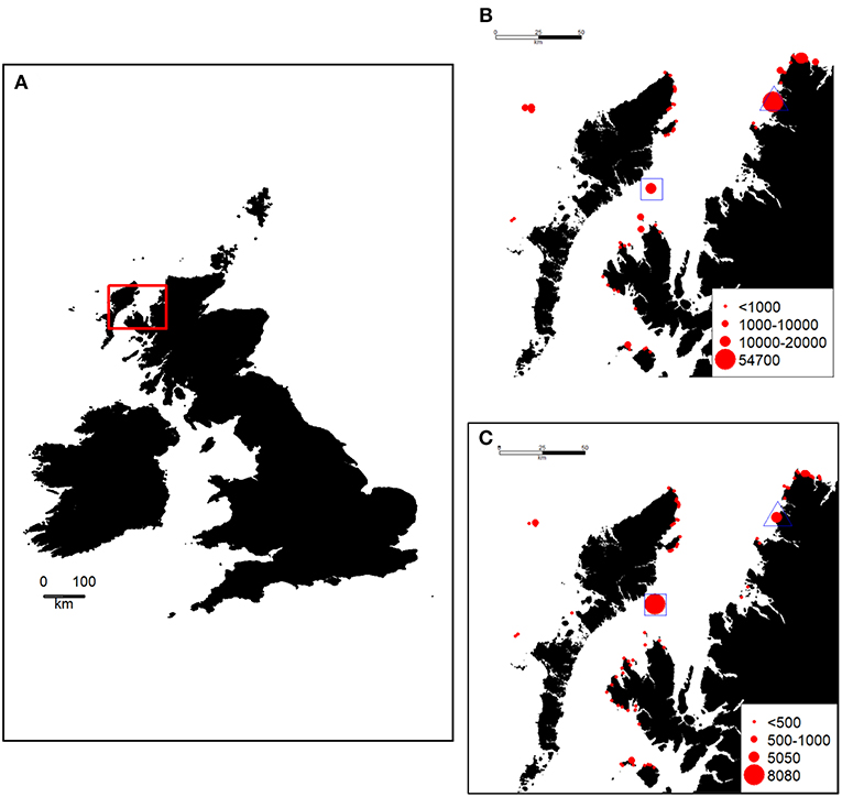
Figure 1. (A) Location of the study area (red box) in the British Isles, size of Guillemot (B) and Razorbill (C) colonies in and around the study area [estimated number of individuals, from the Seabird Monitoring Programme Database www.jncc.gov.uk/smp (Mitchell et al., 2004). During the study, these species were GPS-tracked from a colony on the Shiants (blue square). At the same time, a boat-based survey was undertaken throughout the study area as shown in Figure 3. The location of Handa Island is indicated by a blue triangle.

Data Collection

Tracking Data

Razorbills and guillemots breeding on the Shiants were tracked using an adapted version of the open-source Mataki tag platform (http://mataki.org/) manufactured by debug innovations, Cambridge, with additional programming and construction also required. Unlike archival GPS tags, they do not need to be recovered to retrieve data, which is wirelessly transmitted periodically to base stations. Birds tending eggs or small chicks were caught on the nest using a wire noose or by hand, and tags were attached to back feathers using waterproof Tesa^® tape. Tag mass was 19 g, equivalent to <3.2% body weight of razorbills and <2.3% body weight of guillemots. Between the 7th and 23rd of June (Figure 2), tags were deployed on 20 guillemots and 39 razorbills. Prior to deployment, the battery performance on the Mataki tag was not well-known. Hence, three different temporal tracking resolutions were used in the field: One fix every 100 s (analyses based upon 2 guillemots, 7 razorbills), 200 s (10 guillemots, 18 razorbills), or 600 s (6 guillemots, 8 razorbills).

FIGURE 2

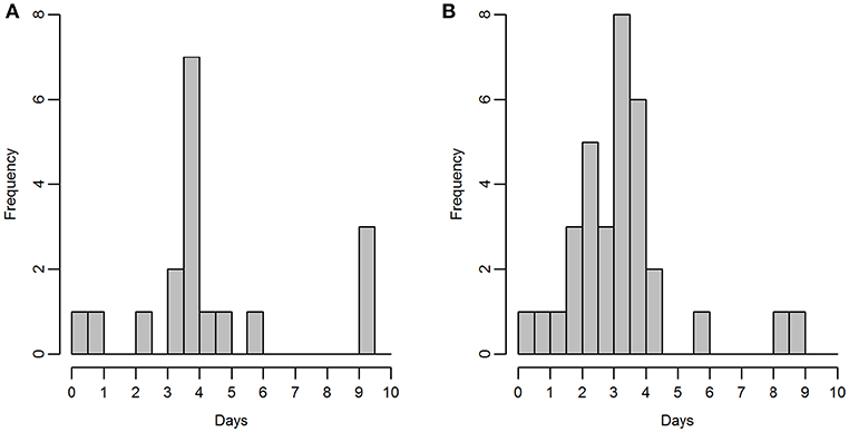
Figure 2. Duration of time for which tags were active, for (A) guillemot and (B) razorbill; bins represent half days.

At-Sea Survey Data

Boat-based surveys using the standard European Seabirds At Sea (ESAS) methodology (Camphuysen et al., 2004) were carried out throughout the Minch (an area of c. 6,700 km²) on 8 days between 9 and 24 June 2015. In brief, the survey was carried out by experienced, ESAS-qualified, seabird surveyors (EW, DS, and SP). The observer searched for all birds flying or sitting on the water within 300 m of one side of the transect line, while a second person recorded sightings. One surveyor generally observed for an entire transect, except on very long transects, resulting in a median shift of 56 min (range 12–177 min). The side of the transect line surveyed was chosen on a transect-by-transect basis to cater for environmental effects (glare, etc.) on detectability. Birds were recorded in 1-min bins, corresponding to a mean distance of 250 m (±21 m SD) traveled. Birds first detected on the water were recorded in one of four distance bands running parallel to the boat's track: A 0–50 m, B 50–100 m, C 100–200 m, and D 200–300 m from the track line. Birds in flight were not recorded in distance bands as their detectability varies little within the 300 m transect. However, a “snapshot” method was used to account for the flux of birds through the transect (Tasker et al., 1984). Birds in flight were recorded as being in the transect if they were within a 300 × 300 m box at a given time interval, with an audible countdown timer being used to prepare the observer to undertake the snapshot instantaneously to reduce bias associated with a protracted snapshot (Gaston et al., 1987). The interval was set according to the boat's speed such that it occurred with every 300 m of transect covered. Transects were primarily aligned north-south and east-west (Figure 3). In addition, sea state, wind direction and strength, precipitation, and visibility were recorded at regular intervals. Surveys were only undertaken in sea states ≤ 4.

FIGURE 3

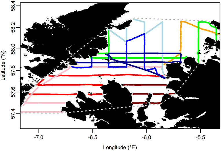
Figure 3. Transects carried out on at-sea surveys. Each color represents a different day of the survey. Gray dotted line encompasses the area over which indices of similarity between at-sea and tracking based distributions were calculated.

Data Analysis

Tracking Data

To achieve a common temporal resolution across birds, all tracks were first rediscretised to a 600-second interval using linear interpolation in the “adehabitatLT” R package (Calenge, 2006). Locations were projected in Lambert azimuthal equal area projection. Locations within 500 m of each bird's nest and all location records falling on land were removed. Kernel density estimation (Worton, 1989), implemented in the “adehabitatHR” R package (Calenge, 2006) with a bivariate Gaussian kernel was then used to determine the utilization distributions (UDs) of the tracked birds. Grid resolution was set to 2 × 2 km and the smoothing parameter h was selected using the ad hoc method (least-squares cross-validation was trialed but failed to converge). The degree to which the sample of birds tracked represented the wider colony was tested using the procedures of Lascelles et al. (2016). Razorbills were better represented than were guillemots, but both datasets were sufficiently representative.

In order to examine whether potential discrepancies between distributions were due to boat surveys being restricted to hours of daylight and calm sea states, UDs were produced using subsets of tracking data. These comprised (1) all data, (2) daytime data, (3) night-time data, and (4) tracking data recorded at the same time as the boat survey was being conducted (i.e., in daylight and weather conditions suitable for visual survey—hereafter contemporary data).

At-Sea Survey Data

Transects were divided into segments of length corresponding to 1 min of survey time. Density (counts/unit area in each segment) was then modeled as a function of a 2-dimensional spatial spline. Methods followed Bradbury et al. (2014), with the exception that distance correction and density surface modeling were carried out in two separate steps as described by Miller et al. (2013). The detectability of birds on the water decreases with distance so the first stage was to apply a factor to correct for the proportion of birds not detected in the 300 m transect. Following Kober et al. (2010), the corrected abundance x was calculated for each species using Equation 1:

$\begin{array}{ll}x=\frac{(nA+nB)\times 3}{(nA+nB+nC+nD)},& (1)\end{array}$

where nA, nB, nC, and nD are the total counts in each distance band. The numerator is multiplied by 3 (the ratio of total area of bands A+B+C+D to total area of bands A+B) (Pollock et al., 2000). This assumes that detection within 100 m of the boat is perfect. As in Kober et al. (2010), correction factors were calculated separately for sea states 0 (very calm) and 1–3 (ripples to wavelets, small whitecaps); unlike in Kober et al. (2010), no calculations were made for sea states 4–5, as very little survey effort was carried out above sea state 3. Correction factors are presented in Table 1. Abundances of birds on the water were multiplied by the appropriate correction factor, and then added to counts of birds in flight (assumed to have perfect detection) to give a total abundance in each transect segment (Figure 4).

TABLE 1

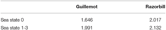
Table 1. Correction factors applied to counts of seabirds detected on the water within a 300 m wide transect during the at-sea survey.

FIGURE 4

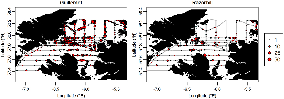
Figure 4. Raw abundances from at-sea surveys, after distance correction.

In the second step, spatial variations in distance-corrected abundances were modeled using generalized additive mixed models (GAMMs) fitted in the “mgcv” R package (Wood, 2003, 2011, 2017). A negative binomial error structure and log link function were specified. “Transect” and “hour-within-transect” were treated as random effects in an attempt to model spatial and temporal clustering of observations (Zuur et al., 2014). An offset of log(segment length) was also included to account for slight variation in the distances traveled each minute (Miller et al., 2013). The fixed effect in each GAMM. The fixed effect in each GAMM were coordinates (eastings and northings), which were combined into a 2-dimensional and continuous variable. The maximum basis dimension (k) for the spline was selected by fitting a range of k values and examining resulting models' Akaike Information Criterion (AIC) values; the final value selected was 150, which represented the point at which adding further complexity provided no further AIC improvements. After model fitting, density was predicted on the same 2 km grid used for UD estimation. Grid cells containing land were excluded from predictions. Hereafter, we assume that the mean proportion of time that birds use a location within the study area is approximately proportional to density predicted from the at-sea survey data. Hereafter, we therefore refer these grids, normalized to sum to one, as UDs. Although there are potential theoretical objections to this interpretation, we assume it here pragmatically, as it allows similarity between the density estimates made using the two methods to be calculated using well-established metrics (Sansom et al., 2018).

Spatial autocorrelation was present in model residuals for both species. However, when an exponential spatial correlation structure was added (using the “gamm” function, and penalized quasi likelihood), for guillemots there was no significant difference in predicted densities. For razorbills, the model did not converge. It was therefore considered impractical to further reduce residual spatial autocorrelation.

Comparing Estimated Distributions

To compare the distribution of birds estimated using tracking data and at-sea survey data, density grids were clipped to a focal area. First, this was defined by the minimum convex polygon (MCP) encompassing the at-sea surveys (Figure 3). The most north-easterly transects occurred within 20 km of the major guillemot and razorbill colony on Handa Island (Figure 1), which could strongly influence seabird distributions in the region. Therefore, a second focal area was considered, defined by a circle centered on the Shiants with a 50 km radius, approximately representing 1.1 x the maximum foraging range of each species observed in our study. Results using the 50 km radius area were nearly identical to those using the MCP area and are not therefore discussed further.

Densities outside the focal area were set to NA and density values within the focal area were then normalized to sum to unity once more. The similarity and overlap of different UDs (nominally, UD₁ and UD₂ in the descriptions below) were then calculated using indices described by Fieberg and Kochanny (2005). First, the 95 and 50% core areas (CAs) were calculated, i.e., the areas in which 95 and 50% usage is expected to occur, and plotted where these overlapped between UD₁ and UD_2. The area of overlap between core areas of UD₁ and UD₂ was then expressed both as a percentage of the area of UD₁, and as a percentage of the area of UD₂. Secondly, the Spearman correlation coefficient (ρ) between the ranks of probability densities in UD₁ and UD₂ was calculated (White and Garrott, 1990). Equal values within UDs were assigned the mean of the rank of those values. Whilst this measure may be limited in identifying overlap of UDs (Fieberg and Kochanny, 2005), it is a simple and widely understood measure of similarity. Positive correlation coefficients indicate that UDs are similar, whilst negative correlation coefficients indicate that higher densities in one UD are matched by lower densities in the other. ρ was calculated across the entire focal area.

Finally, two metrics were calculated, which it has been demonstrated give more reliable estimates of UD overlap (Fieberg and Kochanny, 2005). The utilization distribution overlap index (UDOI) is calculated following Equation 2:

$\begin{array}{ll}{UDOI=A}_{1,2}{\displaystyle {\int }_{-\infty }^{\infty }}{\displaystyle {\int }_{-\infty }^{\infty }}U{D}_1(x,y)\times U{D}_2(x,y)dxdy& (2)\end{array}$

where, A_1,2 indicates the area of overlap between UD₁ and UD₂, whilst UD₁(x,y) indicates the value of UD₁ at location (x,y). This index shows the amount of overlap relative to two UDs that use the same space and are uniformly distributed: UDs with perfect overlap and uniform probability distributions have UDOI = 1, whereas completely non-overlapping UDs have UDOI = 0. Overlapping UDs with non-uniform yet coincident probability distributions have UDOI > 1. This metric therefore indicates when two UDs show a high concentration of probability in the same area.

The second overlap metric used was Bhattacharyya's Affinity (BA), which is calculated following Equation 3 (Fieberg and Kochanny, 2005):

$\begin{array}{ll}BA={\displaystyle {\int }_{-\infty }^{\infty }}{\displaystyle {\int }_{-\infty }^{\infty }}\sqrt{U{D}_1(x,y)}\times \sqrt{U{D}_2(x,y)}dxdy& (3)\end{array}$

BA is 0 for two non-overlapping UDs, and 1 for identical UDs. This metric indicates overall similarity of UDs. Both UDOI and BA were calculated for the entire focal area.

Results

Tracking Data

Two guillemot tags and six razorbill tags returned no data so were excluded from further analyses, leaving sample sizes of 18 guillemots and 33 razorbills. Tags recorded data for between 6 h and 9.25 days (Figure 2). Mean duration was 105 h (SD ± 61 h) for guillemots and 78 h (SD ± 42 h) for razorbills. The last data were collected for both species on the 27th of June. Rediscretisation and data trimming resulted in 5,246 and 5,769 locations for guillemots and razorbills, respectively. Daytime UDs were estimated using tracking data from 17 guillemots and 31 razorbills (3,229 and 3,500 locations, respectively); night-time UDs from 16 guillemots and 30 razorbills (2,017 and 2,269 locations, respectively); and contemporaneous UDs from 15 guillemots and 24 razorbills (734 and 1,090 locations, respectively). The smoothing parameter h was 2.2 km for guillemots and 2.7 km for razorbills. The raw tracks for both species are shown in Figure 5.

FIGURE 5

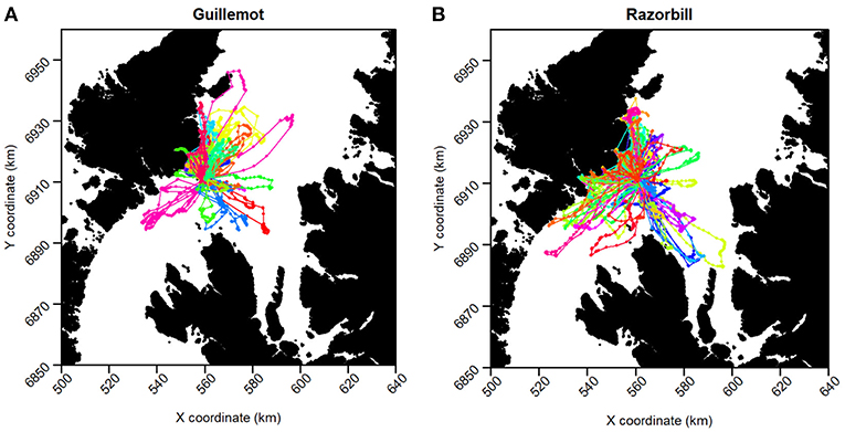
Figure 5. GPS tracks of (A) Guillemot and (B) Razorbill individuals. Each color represents a different individual.

At-Sea Survey Data

The sea state during boat-based surveys was generally low (0 for 9% of the survey, 1 for 23%, 2 for 39%, 3 for 23%, and 4 for 6%) and 950 km of transect was surveyed. In total, 2,338 guillemots (859 in flight, 1,479 on water) and 776 razorbills (453 in flight, 323 on water) were detected (1 and 5% of guillemots/razorbills in flight and on the water respectively, could not be assigned to species and were excluded from the analysis).

Tracking Distributions vs. At-Sea Survey Distributions

Guillemot

Tracking data indicated that the highest guillemot density occurred immediately to the north of the Shiants; lower guillemot densities were spread relatively evenly around the islands (Figure 6A). Guillemot density estimated from boat surveys was spread more evenly and over a larger area, with the highest densities around and to the north of the Shiants, to the north and north-east extremes of the survey area, and off the north-east coast of Skye (Figure 6B).

FIGURE 6

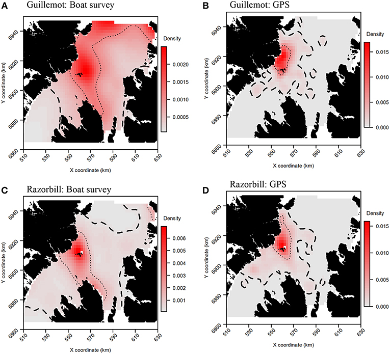
Figure 6. Guillemot (A,B) and Razorbill (C,D) utilization distributions from boat surveys compared with concurrent GPS tracks. Darker reds indicate higher probability densities. Thick, dashed line indicates extent of 95% home range; thin, dotted line indicates extent of 50% home range.

The more even density surfaces from the boat survey meant that core areas (CAs) were much larger, leading to high overlap as a proportion of tracking CAs, but low overlap as a proportion of boat survey CAs (Table 2). Both survey methods found the south-west corner of the survey area to be outside the 95% CA, and the south-west and east regions of the survey area to be outside the 50% CA (Figure 7A). However, whilst tracking CAs were mostly contained within the larger boat survey CAs, tracking CAs were confined to the areas around the Shiants; more distant areas included in boat survey CAs were not included in the tracking CAs (Figure 7A). Similarity indices indicated moderate similarity between UDs estimated from the two data sources (Table 2). Correlation coefficients and BA indicated that boat surveys and GPS produced moderately similar distributions, and UDOI was >1, indicating reasonably good concordance in probability densities.

TABLE 2

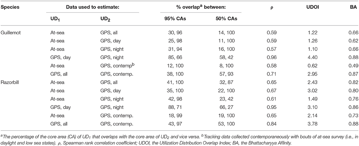
Table 2. Overlap and similarity between seabird utilization distributions (UDs) estimated using data from at-sea surveys and GPS tracking.

FIGURE 7

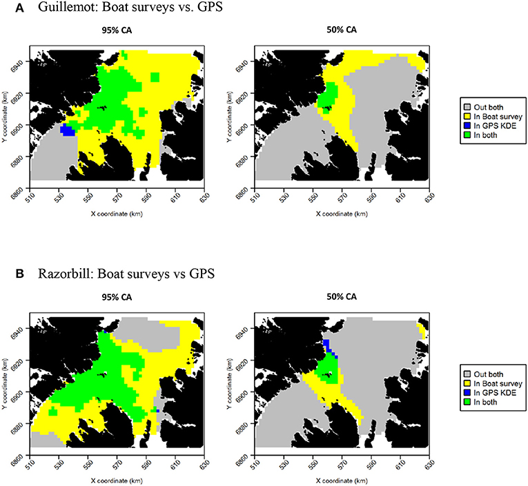
Figure 7. Overlap between guillemot (A) and razorbill (B) core areas (CAs) derived from boat surveys compared with GPS tracking. In both maps, gray indicates areas outside of the CA in both data sources, and green indicates areas inside the CA in both data sources; blue and yellow indicate areas in the CA in one data source but not the other.

Razorbill

For razorbills, the highest densities also occurred primarily to the north of the Shiants (Figures 6C,D). GPS and boat survey distributions indicated an approximate north-west to south-east spread of high density, with this most pronounced in boat survey data, where the 50% CA extended as far as Skye. The pronounced high abundances in the north observed in guillemot distributions were less evident in razorbills, although a likely effect of the colony on Handa in the north-east was again observed. Both GPS and boat survey distributions indicated a low-density area immediately east of the Shiants and low densities in the north.

Core area comparisons were again influenced by the more even, larger distributions derived from boat survey data, with GPS CAs mostly contained within boat survey CAs. However, although boat survey CAs were larger, there was higher spatial concordance with tracking CAs (Table 2), and there appeared to be better concordance visually (Figure 7B). The 95% CAs extended in all directions away from the Shiants, but the tracking derived CA did not extend as far as that derived from the at-sea survey (Figure 7B). The 50% CAs matched well around the Shiants, but the tracking CA did not extend to Skye. Overlap metrics indicated better concordance between the distribution estimates made using tracking and at-sea survey datasets than for guillemots (Table 2). Correlations were again only moderate, but BA > 0.8 and UDOI > 2.4 indicated high similarity between the UDs. The high UDOI statistics are likely to reflect the good matching of high densities found to the north of the Shiants.

Effects of Day/Night on Distribution Similarity

Guillemot

Daytime and night-time distributions were generally similar for guillemots (Figures 8A,B). Both distributions showed the greatest density to occur to the north of the Shiants, but this was more pronounced at night, whilst in daytime the high-density area extended slightly south of the islands. The 95% core area extended over a larger area at night, but both time periods showed the CA to extend in all directions from the islands. Both daytime and night-time core areas were substantially smaller than those derived from at-sea surveys. Consequently, the tracking derived CAs were almost completely contained within the at-sea survey CAs. However, higher proportional overlap was seen with the night-time GPS data (Table 2). The daytime and night-time CAs were very similar, with high overlap and similar spatial distributions (Figure 9). Congruence between at-sea survey and tracking derived UDs was similar, regardless of whether daytime or night-time data were used to derive the latter. All overlap and similarity indices were broadly similar for daytime and night-time data, with neither proving better across all metrics.

FIGURE 8

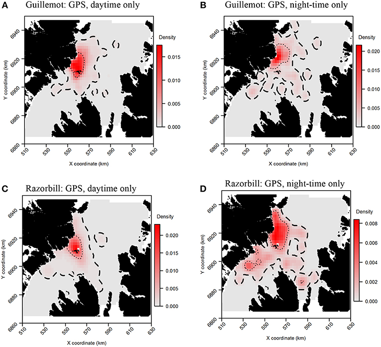
Figure 8. Guillemot (A,B) and Razorbill (C,D) utilization distributions from daytime and night-time subsets of GPS data. Darker reds indicate higher probability densities. Thick, dashed line indicates extent of 95% home range; thin, dotted line indicates extent of 50% home range.

FIGURE 9

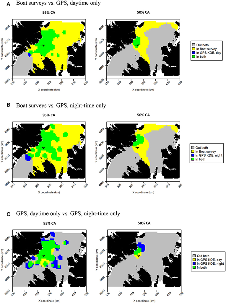
Figure 9. Overlap between guillemot core areas (CAs) derived from boat surveys, GPS tracking in daytime and GPS tracking at night-time. In all maps, gray indicates areas outside of the CA in both data sources, and green indicates areas inside the CA in both data sources; blue and yellow indicate areas in the CA in one data source but not the other. (A) Boat surveys vs. GPS, daytime only. (B) Boat surveys vs. GPS, night-time only. (C) GPS, daytime only vs. GPS, night-time only.

Razorbill

Razorbills showed slightly greater differences between daytime and night-time distributions than guillemots (Figures 8C,D, Table 2). In daytime, the distribution was centered on the Shiants, whilst at night-time, the distribution extended much further to the north. Although the 95% tracking CA extended to Skye at daytime, it extended further in all directions at night-time. Further, the 50% tracking CA extended to a second center at night-time, to the south-west of the Shiants. Tracking vs. at sea survey core area overlap was slightly greater at night-time (Table 2; Figure 10). However, the extension of the 50% tracking CA at night-time to the north-east and south-west of the Shiants was not reflected in the at-sea survey CA. This was the only instance of the tracking data identifying a core area outside that detected indicated by the at-sea data. Perhaps due to the better matching of the 50% CAs derived from at-sea and tracking data, overlap metrics were typically higher when the daytime tracking data were used (Table 2). In particular, UDOI was substantially higher in daytime, suggesting that areas of high density matched well with those identified in boat surveys. BA and correlation values were broadly similar, however, suggesting that both daytime and night-time showed broadly the same patterns overall.

FIGURE 10

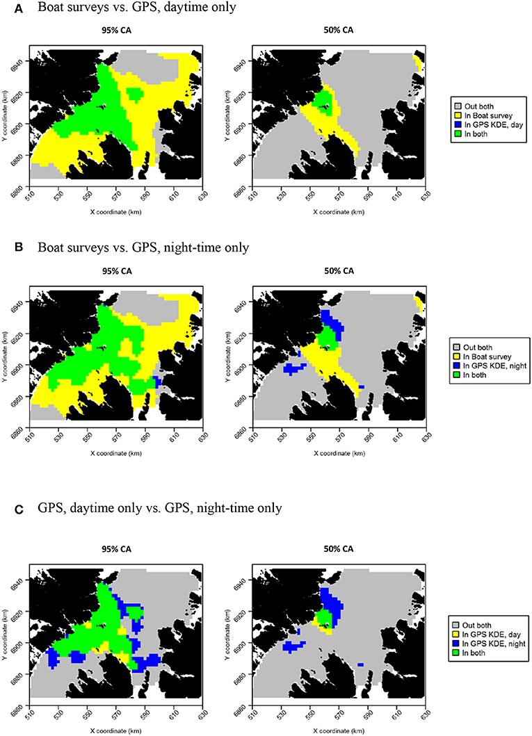
Figure 10. Overlap between razorbill core areas (CAs) derived from boat surveys, GPS tracking in daytime and GPS tracking at night-time. In all maps, gray indicates areas outside of the CA in both data sources, and green indicates areas inside the CA in both data sources; blue and yellow indicate areas in the CA in one data source but not the other. (A) Boat surveys vs. GPS, daytime only. (B) Boat surveys vs. GPS, night-time only. (C) GPS, daytime only vs. GPS, night-time only.

Effects of Temporal Matching on Distribution Similarity

For both species, the tracking UDs derived from data recorded only during bouts of at-sea survey were much smaller than their equivalents derived from the entire tracking data set, presumably due to the smaller number of locations in the former (Figure 11). For guillemots, the highest density was again to the north of the Shiants, but the 95% CA extended north and south of the islands, and was unlike that derived from any other data source. For razorbills, higher densities were centered around the Shiants, with less of the northward bias seen when using the full dataset. For both species, the smaller CAs identified from the subset of tracking data meant that overlap was smaller than when the whole dataset was used (Table 2; Figures 12, 13) and similarity between the tracking and at-sea survey derived UDs was generally lower than when the full tracking data set was used to estimate distributions, although some metrics produced similar values to those seen with the full dataset (Table 2).

FIGURE 11

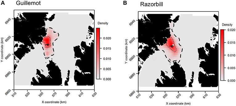
Figure 11. Guillemot (A) and Razorbill (B) utilization distributions from GPS data collected only during times when boat surveys were being carried out. Darker reds indicate higher probability densities. Thick, dashed line indicates extent of 95% home range; thin, dotted line indicates extent of 50% home range.

FIGURE 12

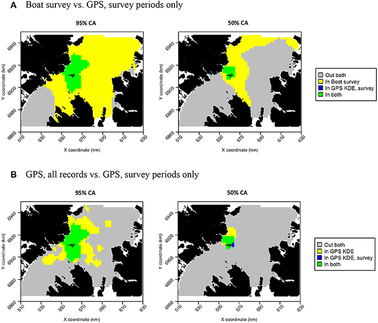
Figure 12. Overlap between guillemot core areas (CAs) derived from boat surveys, GPS tracking during boat survey periods only and all GPS tracking data. In all maps, gray indicates areas outside of the CA in both data sources, and green indicates areas inside the CA in both data sources; blue and yellow indicate areas in the CA in one data source but not the other. (A) Boat survey vs. GPS, survey periods only. (B) GPS, all records vs. GPS, survey periods only.

FIGURE 13

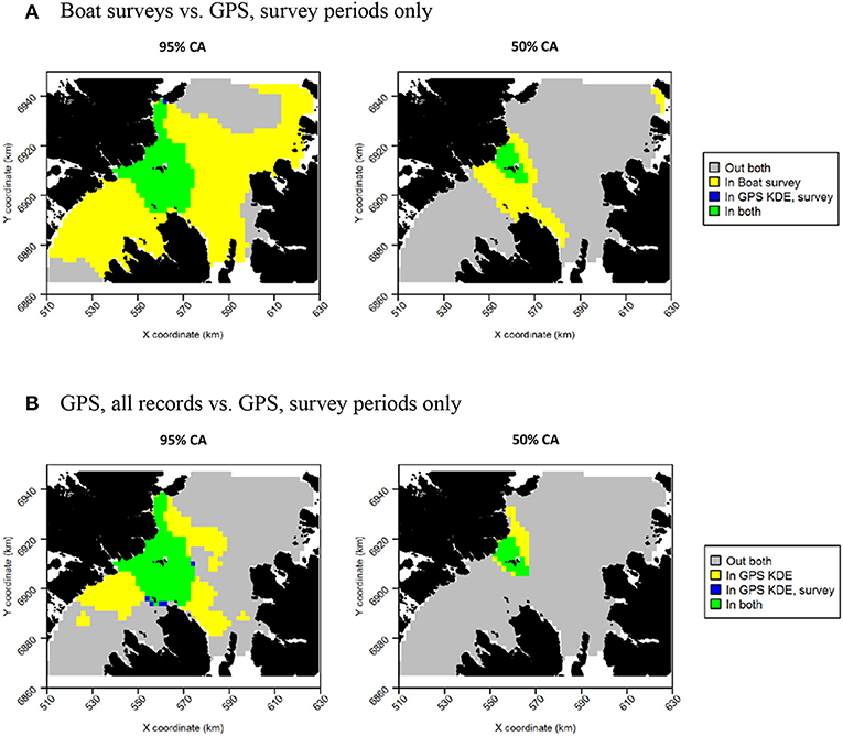
Figure 13. Overlap between razorbill core areas (CAs) derived from boat surveys, GPS tracking during boat survey periods only and all GPS tracking data. In all maps, gray indicates areas outside of the CA in both data sources, and green indicates areas inside the CA in both data sources; blue and yellow indicate areas in the CA in one data source but not the other. (A) Boat surveys vs. GPS, survey periods only. (B) GPS, all records vs. GPS, survey periods only.

Discussion

Similarity Between Different Data Sources

The degree of similarity between seabird distributions derived from boat surveys and GPS tracking differed between the two species: it was moderate for guillemots but somewhat stronger for razorbills. For both species, similarity was greatest close to the Shiants, with boat surveys and GPS tracking both indicating higher densities just to the north of the islands. This was evident for razorbills in particular, for which the two methods showed remarkably good concordance in the location of the 50% core area. However, GPS tracking did not identify areas of high density further away from the islands which were indicated by the boat surveys, particularly in the north of the survey area. For razorbills, moderately high densities near to Skye were suggested from GPS tracking, whereas the boat survey showed this pattern more strongly. However, both data sources agreed well as to locations of low densities, with guillemots in particular present at low densities in the south-west of the survey area and, to a lesser extent, in the east.

When GPS data were sub-sampled to produce daytime and night-time distributions separately, the effect differed slightly between the two species. For guillemots, there was high similarity between day and night, and therefore with the overall GPS distribution. However, for razorbills, day and night distributions differed slightly, with the daytime distribution generally showing a better match to the boat survey distribution.

Boat surveys can only be carried out in daylight and when weather conditions permit, whereas GPS tags record locations in all light and weather conditions. It was anticipated that restricting GPS records to contemporary periods in which boat surveys had been carried out would improve the match to boat survey data. However, the sub-sampled GPS dataset was substantially smaller than when the full dataset was used, so although some similarity metrics indicated similar performance to the full dataset, there appeared to be a somewhat poorer match in general. Indeed, due to the reduced dataset, sample size effects could account for the poorer match.

Potential Reasons for Differences

Limitations of Single-Colony Tracking

One of the most likely causes of differences in distribution from the two data sources was that birds were only tracked from the Shiants, whereas birds observed on boat surveys could originate from other colonies within the study area. Handa Island, lying to the north-east of the study area, supports the largest colonies of guillemots and razorbills in the UK (Mitchell et al., 2004), and is likely to account for the high densities observed in the north of the boat survey area. Indeed, Poisson-kriged distributions from data collected over several decades presented by Kober et al. (2010) also show high densities to occur in the areas identified by boat surveys, suggesting that they are not artifacts of our sampling or analysis. Thus, one major difference in the datasets is that tracking birds from the Shiants cannot indicate the distribution of birds originating from Handa Island. This will likely have been a greater issue for guillemots since Handa supports six times more guillemots than razorbills. This may explain the greater correspondence between GPS tracks and boat survey results for razorbill. The wider distribution of birds, particularly guillemots, closer to Skye detected during boat surveys probably reflected the colonies around Rubha Hunish off the northern tip of Skye. In order to accurately identify wider distributions in a region using GPS tracking, it would be necessary to track birds from multiple major colonies, to produce a predictive model to estimate likely distribution of birds from all colonies in the region (e.g., Wakefield et al., 2017).

Data Resolution and Sampling Effort

Boat survey methodology could also have contributed to differences. The temporal and spatial resolution of survey transects can influence the resolution of the resulting distributions (Camphuysen et al., 2004). Coarser resolutions might allow larger areas to be surveyed, but will limit the ability to identify fine-scale distribution patterns. Conversely, the high accuracy, frequent records obtained from GPS tracking enable finely-resolved distributions to be estimated. Some of the differences found here may result from the difference in resolution of the input data; for example, this could be responsible for differences in the shape of 95% CAs to the north of the Shiants. Further, boat survey findings are highly sensitive to temporal variation in abundances within days and seasons (Camphuysen et al., 2004). This is perhaps most strongly illustrated by the presence of a flock on a transect, which would cause a very high abundance to be recorded, but which may not be present if the transect were repeated, even a short time later. Repeat sampling of transects (Camphuysen et al., 2004) or use of data from multiple surveys (e.g., Kober et al., 2010; Bradbury et al., 2014) would reduce the influence of short term temporal fluctuations in abundance, but with inevitable increase in survey costs per unit area.

A further consideration of sampling effort is the colony-level representativeness of the sample of birds tracked. The 31 razorbills and 17 guillemots included in kernel density estimates represent a tiny fraction of their respective populations on the Shiants (c. 0.4% of razorbills and 0.1% of guillemots). It may therefore also be the case that for guillemots, where the proportion and absolute number of birds tracked was smaller, resulting distributions were less representative of the colony as a whole. Indeed, the number of birds, and the number of trips carried out by each bird, influences resulting home range estimates (Soanes et al., 2013), so sample size effects may contribute to the differences in distributions between data sources (see sensitivity analysis in Carroll et al., 2017).

Sampling Constraints

Differences in the time of day and sea states when sampling is conducted is also an important consideration. GPS tracking typically occurs continuously once the tag is attached, thus sampling locations in all light and weather conditions. Conversely, boat surveys can only take place in the daytime and in good weather and consequently represent distributions during these conditions. However, in this study sub-setting GPS datasets to be contemporary with boat survey data did not consistently result in greater similarity of distributions. The potential improvement in similarity may be offset to some degree by the counteracting effect of reduction in the sample size of GPS records, leading to sparser distributions and a poorer representation of the colony distribution. For guillemots, there was little difference between night and day GPS distributions, and sub-setting to contemporary locations did not improve the similarity to boat surveys. The similarity between day and night GPS distributions, and the similar match of both to boat survey data suggests that there may therefore be little bias associated with conducting boat surveys during daylight on estimated guillemot distributions. On the other hand, for razorbills, night-time and daytime GPS distributions showed greater differences, and the daytime GPS distribution showed greater similarity (measured by UDOI) with boat surveys, as expected. Further sub-setting of GPS data to contemporary locations decreased the similarity with boat survey data, likely to due to reduced sample size.

Biases in at Sea Survey Data

Surveying birds from boats can result in multiple sources of error in density estimates (Gaston et al., 1987; Hyrenbach, 2001; Ronconi and Burger, 2009). Due to the study design and the conditions under which the data were collected, the errors should have been uniformly distributed throughout the study area and therefore should not have introduced systematic bias in the boat-based UD estimates. For example, while the ability to detect birds may have differed among observers and weather conditions, observer effort was spread evenly throughout the survey area and weather conditions were good throughout the survey. Hence, we think it unlikely that systematic biases in at-sea data collection could have accounted for the observed differences in the at-sea and tracking based UDs.

Breeding and Behavioral Status of Sampled Individuals

It is also important to consider the breeding status, and hence time budget and central place foraging constraints, of the individuals sampled. Due to practical limitations in approaching and capturing birds, GPS tracking is most frequently carried out on breeding individuals. Conversely, boat surveys sample all birds at sea, regardless of breeding status. If breeders, non-breeders and failed breeders share the same habitat preferences, there may be little impact of sampling bias in breeding status on resulting distributions. However, there may be important differences in the distributions of breeding and non-breeding individuals. Notably, non-breeders do not need to return to the colony to fulfill nest-attendance functions so can travel further (e.g., Votier et al., 2011). Breeding adults and immatures may also have dietary differences (Campioni et al., 2016) leading to them foraging in different areas (e.g., Fayet et al., 2015). The overall impact of this on estimated distributions depends on the proportion of the total population comprising non-breeders: fewer non-breeders would make distributions from boat surveys and GPS tracking appear more similar. It has been estimated that there are around 0.74-0.75 non-breeding immatures per adult at guillemot and razorbill breeding colonies (Furness, 2015). However, breeding age adults may skip breeding in some years: on the Isle of May, 5-10% of guillemots around the colony each year did not breed (Harris and Wanless, 1995), and the rate of skipping breeding can vary (e.g., Reed et al., 2015). Therefore, the presence of immatures and non-breeding adults in the at-sea population sampled by boat surveys could lead to differences with GPS-derived distributions; developing our understanding of the distributions on non-breeders at sea will be an important step in addressing this issue.

Breeding stage can also influence the distribution of seabirds at sea, due to difference in the constraints on nest attendance operating during incubation, brood-guard and post-guard periods (e.g., Wakefield et al., 2011; Dean et al., 2015). When selecting individuals for tag deployment, no attempt was made to target birds at a particular breeding stage and it is likely that the breeding stage of the tracked individuals reflected that of the colony as a whole. Hence the breeding stage of the birds observed from contemporaneous boat surveys is likely to be similar to that of the tracked sample.

In our study, we did not attempt to discriminate differences in the distribution of birds in different behavioral states. Whilst away from the colony on foraging trips, guillemots and razorbills rearing small chicks tracked in the North Sea spent 28.8 ± 9.5 and 17.5 ± 10.6% (mean ± sd) of their time, respectively underwater (Thaxter et al., 2010). Dive times average 46.4 ± 27.4 and 50.4 ± 7.4 s for guillemots during long and short dives, respectively and 23.1 ± 14.9 s for razorbills, which made only short dives. The average boat speed in our survey was 14 ± 3 km/h, so guillemots and razorbills would have been out of sight during dives for on average the time it took to traverse ~190 and 90 m of transect, respectively. This effect could have been further exacerbated if auks dived to escape the approaching survey vessel, although it is our experience that common guillemots and razorbills only respond in this way when the vessel is very close and they are likely to have already been detected. Nonetheless, it is likely that up to around 29% of guillemots and 18% of razorbills would not have been detected during the boat survey, leading to a concomitant underestimate of density (Buckland et al., 2015). This would have biased the boat based UDs lower in foraging areas, causing a systematic bias if foraging behavior was distributed non-uniformly. Although GPS loggers do not record locations while birds are diving, the interpolation scheme we used to fill gaps in the GPS data would have greatly reduced any similar bias in the tracking-based UDs. Hence, the spatial bias in the boat-based but not tracking-based UDs could partially explain why the latter suggested higher bird densities close to the Shiants than the former (Figure 4), i.e., breeding birds could have been diving intensively in an annulus around the colony Ashmole's halo (Gaston et al., 2007) and therefore missed more frequently than for example, non-breeders foraging less intensively at a greater distance.

Data Types and Analytical Approaches

Tracking individuals over time, and counting the abundance of birds along transects at sea, represent two very different types of data. The analytical processes required to estimate densities from such data are extremely different, and rely on different assumptions. Differences in the distributions resulting from the two methods may therefore be due, in part, to differences in the data types and the differences in the ways in which they are processed. Furthermore, there is no standard approach to converting raw survey data into a continuous density surface. Accordingly, various methods have been used, and the differences between these methods could contribute to perceived differences in resulting distributions. Such effects were noted by Bradbury et al. (2014) “The Poisson kriging method used by Kober et al. gave more scattered discreet [sic areas of higher density whereas the DSM of this study generally gave wider smooths over areas.” Analytical differences could be particularly acute in the present study, where GPS distributions reflect the raw data, whereas boat survey distributions were modeled. One consequence of this is that zero values occur rarely in modeled boat survey distributions, whereas they occur across large areas in GPS distributions; this alone may influence overlap metric scores. Had it been possible to replicate the Poisson kriging method of Kober et al. (2010), the patchier densities may have matched GPS distributions better. Other analytical considerations will also have influenced resulting distributions. The form of spatial smooth used in GAMMs can affect outputs; a large maximum basis dimension was selected based on AIC, thus allowing a relatively complex distribution to be modeled, but similar studies have used simpler splines (e.g., Winiarski et al., 2013) or different forms of splines (e.g., Bradbury et al., 2014). In GPS distributions, the smoothing parameter used in kernel density estimation influences the size and shape of resulting core areas, with the rule-of-thumb method producing larger, smoother kernels than least-squares cross-validation or the plug-in method (Walter et al., 2011).

There are a number of analytic approaches that could further help in a comparison of distributions generated from tracking with those from boat surveys in this region. It would be beneficial to explicitly examine the sensitivity of KDEs derived from GPS data. The first step would be to restrict the number of birds and data points included, to explicitly consider sample size effects. This would be used to examine two questions: first, whether the larger sample of birds is likely to be responsible for the better matching of razorbill than guillemot distributions, and second, whether reduced sample sizes caused poorer matching in the comparisons with contemporary GPS and boat survey data. The second step would be to examine the methods used for producing KDEs, trialing plug-in estimators for the smoothing parameter and trialing Brownian bridge movement models. Although these different methods should not produce substantially different results, understanding the degree to which these assumptions affect distributions would be informative.

After understanding KDE sensitivity, it would be beneficial to model GPS data rather than simply estimating kernel densities from the raw data. Since boat survey data were modeled as a function of spatial location, using a similar approach for GPS data would allow closer matching of methods. However, this is not straightforward: different modeling approaches are available, with Wakefield et al. (2017) using a Poisson point-process method using only presence data, and other analyses (Wakefield et al., 2012; Wilson et al., 2014; Cleasby et al., 2015) using a “case-control” approach whereby observed presences are matched by “pseudo-absences.” Each method brings with it complexities and assumptions, so could introduce further analytical reasons for observed differences. However, modeling GPS data, which would likely provide smoother core area estimates, would allow examination of the degree to which differences are driven by analytical method.

Once a predictive model structure for GPS data has been established, it would be possible to introduce habitat predictor variables to both GPS and boat survey models. Distributions may be better modeled by considering the habitat variables that determine which areas the birds use (see Wakefield et al., 2017). This approach should also allow predictions to be made beyond the Shiants for GPS data. On the other hand, inclusion of habitat variables could also introduce artifacts as distributions become related to spatially-variable predictors.

Conclusions

Similarities in core-areas of animals from the focal colony were obtained, but suspected influences of neighboring colonies and non-breeders are apparent in differences between methods. The magnitude of differences is linked to the relative sizes of these populations—being larger in common guillemots where neighboring colonies were considerably larger than the focal colonies. These results support the use of GPS loggers for defining distributions of species in certain regions, but only when neighboring colonies are neither large nor widespread. Therefore, these results support the use of a flexible approach tailored to the needs of the study. Distributions of animals around isolated colonies could be achieved using GPS loggers but that of animals around aggregated colonies is best suited to at-sea surveys or multi-colony tracking.

Data Availability

The datasets for this manuscript are not publicly available as yet because they are being used for an upcoming publication comparing seabird and cetacean distributions in the study. Requests to access the datasets should be directed to MB at mark.bolton@rspb.org.uk. The tracking dataset will subsequently be available from http://www.seabirdtracking.org/.

Ethics Statement

This study was carried out in accordance with the principles of the UK Animals (Scientific Procedures) Act 1986. Capture, handling and tagging of birds was carried out under all appropriate licenses, issued by the British Trust for Ornithology, on behalf of the UK Government Home Office.

Author Contributions

PE and MB initiated this collaboration, conceived the project, and obtained the funding. EO developed the tags and organized the tracking of birds on the Shiants, which was undertaken by ES. PE organized and led the boat surveys in which JW participated and EW and SP undertook field observations. MC conducted the analyses, prepared the figures and tables, and wrote an initial draft of the paper. All authors provided critical feedback on the manuscript. PE prepared the final manuscript and handled the submission.

Funding

The study was funded by the UK Government Department of Energy and Climate Change (DECC, now the Department for Business, Energy and Industrial Strategy) under the Offshore Energy Strategic Environmental Assessment programme (OESEA-15-54), the Sea Watch Foundation, and RSPB. EW is funded by the Natural Environment Research Council (Independent Research Fellowship NE/M017990/1).

Conflict of Interest Statement

The authors declare that the research was conducted in the absence of any commercial or financial relationships that could be construed as a potential conflict of interest.

Acknowledgments

We thank John Hartley (Hartley Anderson Ltd.) for project management on behalf of DECC; Pia Anderwald, Jerry Gillham, Kathy James, Ali MacLennan, David Shackleton, Tom Stringell, Gemma Veneruso, and Caroline Weir for assistance with the vessel surveys; the Shiants Auk Ringing Group for field assistance on the Shiants; Andrew Asque and Nigel Butcher for development of the tags, David Lambie for boat charter and assistance; and Tom and Adam Nicolson for permission to work on the Shiants. Fieldwork was conducted under license from Scottish Natural Heritage and the British Trust for Ornithology.

References

Bradbury, G., Trinder, M., Furness, B., Banks, A. N., Caldow, R. W., and Hume, D. (2014). Mapping seabird sensitivity to offshore wind farms. PLoS ONE 9:e106366. doi: 10.1371/journal.pone.0106366

PubMed Abstract | CrossRef Full Text | Google Scholar

Buckland, S. T., Burt, M. L., Rexstad, E. A., Mellor, M., Williams, A., and Woodward, R. (2012) Aerial surveys of seabirds: the advent of digital methods. J. Appl. Ecol. 49, 960–967. doi: 10.1111/j.1365-2664.2012.02150.x

CrossRef Full Text | Google Scholar

Buckland, S. T., Rexstad, E. A., Marques, T. A., and Oedekoven, C. S. (2015). Distance Sampling: Methods and Applications. Cham: Springer International Publishing.

Google Scholar

Burger, A. E., and Shaffer, S. A. (2008). Application of tracking and data-logging technology in research and conservation of seabirds. Auk 125, 253–264. doi: 10.1525/auk.2008.1408

CrossRef Full Text | Google Scholar

Calenge, C. (2006). The package adehabitat for the R software: a tool for the analysis of space and habitat use by animals. Ecol. Modell. 197, 516–519. doi: 10.1016/j.ecolmodel.2006.03.017

CrossRef Full Text | Google Scholar

Camphuysen, C. J., Fox, A. D., Leopold, M. F., and Petersen, I. K. (2004). Towards Standardised Seabirds at Sea Census Techniques in Connection With Environmental Impact Assessments for Offshore Wind Farms in the UK: A Comparison of Ship and Aerial Sampling Methods for Marine Birds and Their Applicability to Offshore Wind Farm Assessments. Texel: Royal Netherlands Institute for Sea Research.

Google Scholar

Campioni, L., Granadeiro, J. P., and Catry, P. (2016). Niche segregation between immature and adult seabirds: does progressive maturation play a role? Behav. Ecol. 27, 426–433. doi: 10.1093/beheco/arv167

CrossRef Full Text | Google Scholar

Carroll, M. J., Wakefield, E. W., Scragg, E. S., Pinder, S., Shackleton, D., Owen, E., et al. (2017). Supplement 1: Representativeness Testing of GPS Tracking Data. Sandy: Royal Society for the Protection of Birds.

Google Scholar

Chivers, L. S., Lundy, M. G., Colhoun, K., Newton, S. F., Houghton, J. D. R., and Reid, N. (2013). Identifying optimal feeding habitat and proposed Marine Protected Areas (pMPAs) for the black-legged kittiwake (Rissa tridactyla) suggests a need for complementary management approaches. Biol. Conserv. 164, 73–81. doi: 10.1016/j.biocon.2013.04.022

CrossRef Full Text | Google Scholar

Cleasby, I. R., Wakefield, E. D., Bodey, T. W., Davies, R., Patrick, S. C., Newton, J., et al. (2015). Sexual segregation in a wide-ranging marine predator is a consequence of habitat selection. Mar. Ecol. Prog. Ser. 518, 1–12. doi: 10.3354/meps11112

CrossRef Full Text | Google Scholar

Dean, B., Kirk, H., Fayet, A., Shoji, A., Freeman, R., Leonard, K., et al. (2015). Simultaneous multi-colony tracking of a pelagic seabird reveals cross-colony utilization of a shared foraging area. Mar. Ecol. Prog. Ser. 538, 239–248. doi: 10.3354/meps11443

CrossRef Full Text | Google Scholar

Fayet, A. L., Freeman, R., Shoji, A., Padget, O., Perrins, C. M., and Guilford, T. (2015). Lower foraging efficiency in immatures drives spatial segregation with breeding adults in a long-lived pelagic seabird. Anim. Behav. 110, 79–89. doi: 10.1016/j.anbehav.2015.09.008

CrossRef Full Text | Google Scholar

Fieberg, J., and Kochanny, C. O. (2005). Quantifying home-range overlap: the importance of the utilization distribution. J. Wildl. Manag. 69, 1346–1359. doi: 10.2193/0022-541X(2005)69[1346:QHOTIO]2.0.CO;2

CrossRef Full Text | Google Scholar

Furness, B. (2015). Non-breeding Season Populations of Seabirds in UK Waters: Population Sizes for Biologically Defined Minimum Population Scales (BDMPS). Natural England Commissioned Report number 164. Natural England, Peterborough.

Google Scholar

Gaston, A. J., Collins, B. L., and Diamond, A. W. (1987). The “snapshot” count for Estimating densities of flying seabirds during boat transects: a cautionary comment. Auk Ornithol. Adv. 104, 336–338.

Google Scholar

Gaston, A. J., Ydenberg, R. C., and Smith, G. E. J. (2007). Ashmole's halo and population regulation in seabirds. Mar. Ornithol. 35, 119–126.

Google Scholar

Gjerdrum, C., Fifield, D. A., and Wilhelm, S. I. (2012). Eastern Canada Seabirds at Sea (ECSAS) Standardized Protocol for Pelagic Seabird Surveys From Moving and Stationary Platforms. Tech. Rep. 515, 37 pp., Can. Wildlife Serv., Atl. Reg., Dartmouth, Nova Scotia. Available online at: http://www.cnlopb.nl.ca/pdfs/hmdcjdb/ecseabird.pdf.

Google Scholar

Grecian, W. J., Lane, J. V., Michelot, T., Wade, H. M., and Hamer, K. C. (2018) Understanding the ontogeny of foraging behaviour: insights from combining marine predator bio-logging with satellite-derived oceanography in hidden Markov models. J. R. Soc. Interface 15:20180084. doi: 10.1098/rsif.2018.0084

PubMed Abstract | CrossRef Full Text | Google Scholar

Harris, M. P., Bogdanova, M. I., Daunt, F., and Wanless, S. (2012). Using GPS technology to assess feeding areas of Atlantic Puffins Fratercula arctica. Ringing Migr. 27, 43–49. doi: 10.1080/03078698.2012.691247

CrossRef Full Text | Google Scholar

Harris, M. P., and Wanless, S. (1995). Survival and non-breeding of adult common guillemots Uria aalge. Ibis 137, 192–197. doi: 10.1111/j.1474-919X.1995.tb03239.x

CrossRef Full Text | Google Scholar

Hyrenbach, K. D. (2001). Albatross response to survey vessels: implications for studies of the distribution, abundance, and prey consumption of seabird populations. Mar. Ecol. Prog. Ser. 212, 283–295. doi: 10.3354/meps212283

CrossRef Full Text | Google Scholar

Kober, K., Webb, A., Win, I., Lewis, M., O'Brien, S., Wilson, L., et al. (2010). An Analysis of the Numbers and Distribution of Seabirds Within the British Fishery Limit Aimed at Identifying Areas That Qualify as Possible Marine SPAs. JNCC Report 431, JNCC, Peterborough, UK.

Google Scholar

Lascelles, B. G., Taylor, P. R., Miller, M. G. R., Dias, M., Oppel, S., Torres, L., et al. (2016). Applying global criteria to tracking data to define important areas for marine conservation. Divers. Distrib. 22, 422–431. doi: 10.1111/ddi.12411

CrossRef Full Text | Google Scholar

Louzao, M., Bécares, J., Rodríguez, B., Hyrenbach, K. D., Ruiz, A., and Arcos, J. M. (2009). Combining vessel-based surveys and tracking data to identify key marine areas for seabirds. Mar. Ecol. Prog. Ser. 391, 183–197. doi: 10.3354/meps08124

CrossRef Full Text | Google Scholar

Miller, D. L., Burt, M. L., Rexstad, E. A., and Thomas, L. (2013). Spatial models for distance sampling data: recent developments and future directions. Methods Ecol. Evol. 4, 1001–1010. doi: 10.1111/2041-210X.12105

CrossRef Full Text | Google Scholar

Mitchell, P. I., Newton, S. F., Ratcliffe, N., and Dunn, T. E. (2004). Seabird Populations of Britain and Ireland. London: T & AD Poyser.

Google Scholar

Phillips, R. A., Silk, J. R. D., Phalan, B., Catry, P., and Croxall, J. P. (2004) Seasonal sexual segregation in two Thalassarche albatross species: competitive exclusion, reproductive role specialization or foraging niche divergence? Proc. R. Soc. Lond. B 271, 1283–1291. doi: 10.1098/rspb.2004.2718

PubMed Abstract | CrossRef Full Text | Google Scholar

Pollock, C. M., Mavor, R., Weir, C. R., Reid, A., White, R., Tasker, M. L., et al. (2000). The Distribution of Seabirds and Marine Mammals in the Atlantic Frontier, North and West of Scotland. 1861075057, Peterborough: JNCC.

Google Scholar

Redfern, C. P. F., and Bevan, R. M. (2014). A comparison of foraging behaviour in the North Sea by Black-legged Kittiwakes Rissa tridactyla from an inland and a maritime colony. Bird Study 61, 17–28. doi: 10.1080/00063657.2013.874977

CrossRef Full Text | Google Scholar

Reed, T., Harris, M., and Wanless, S. (2015). Skipped breeding in common guillemots in a changing climate: restraint or constraint? Front. Ecol. Evol. 3:1. doi: 10.3389/fevo.2015.00001

CrossRef Full Text | Google Scholar

Robertson, G. S., Bolton, M., Grecian, W. J., and Monaghan, P. (2014). Inter- and intra-year variation in foraging areas of breeding kittiwakes (Rissa tridactyla). Mar. Biol. 161, 1973–1986. doi: 10.1007/s00227-014-2477-8

PubMed Abstract | CrossRef Full Text | Google Scholar

Ronconi, R. A., and Burger, A. E. (2009). Estimating seabird densities from vessel transects: distance sampling and implications for strip transects. Aquat. Biol. 4, 297–309. doi: 10.3354/ab00112

CrossRef Full Text | Google Scholar

Sansom, A., Wilson, L. J., Caldow, R. W. G., and Bolton, M. (2018) Comparing marine distribution maps for seabirds during the breeding season derived from different survey and analysis methods. PLoS ONE 13:e0201797. doi: 10.1371/journal.pone.020179

PubMed Abstract | CrossRef Full Text | Google Scholar

Soanes, L. M., Arnould, J. P. Y., Dodd, S. G., Sumner, M., and Green, J. A. (2013). How many seabirds do we need to track to define home-range area? J. Appl. Ecol. 50, 671–679. doi: 10.1111/1365-2664.12069

CrossRef Full Text | Google Scholar

Soanes, L. M., Bright, J. A., Angel, L. P., Arnould, J. P., Bolton, M., Berlincourt, M., et al. (2016). Defining marine important bird areas: testing the foraging radius approach. Biol. Conserv. 196, 69–79. doi: 10.1016/j.biocon.2016.02.007

CrossRef Full Text | Google Scholar

Stone, R. E., Webb, A., Barton, C., Ratcliffe, N., Reed, T. C., Tasker, M. L., et al. (1995). An Atlas of Seabird Distribution in North-West European Waters. Peterborough: Joint Nature Conservation Committee.

Google Scholar

Tasker, M. L., Jones, P. H., Dixon, T., and Blake, B. F. (1984). Counting seabirds at sea from ships - a review of methods employed and a suggestion for a standardized approach. Auk 101, 567–577.

Google Scholar

Thaxter, C. B., Wanless, S., Daunt, F., Harris, M. P., Benvenuti, S., Watanuki, Y., et al. (2010). Influence of wing loading on the trade-off between pursuit-diving and flight in common guillemots and razorbills. J. Exp. Biol. 213, 1018–1025. doi: 10.1242/jeb.037390

PubMed Abstract | CrossRef Full Text | Google Scholar

Thomas, L., Buckland, S. T., Rexstad, E. A., Laake, J. L., Strindberg, S., Hedley, S. L., et al. (2010). Distance software: design and analysis of distance sampling surveys for estimating population size. J. Appl. Ecol. 47, 5–14. doi: 10.1111/j.1365-2664.2009.01737.x

PubMed Abstract | CrossRef Full Text | Google Scholar

Votier, S. C., Grecian, W. J., Patrick, S., and Newton, J. (2011). Inter-colony movements, at-sea behaviour and foraging in an immature seabird: results from GPS-PPT tracking, radio-tracking and stable isotope analysis. Mar. Biol. 158, 355–362. doi: 10.1007/s00227-010-1563-9

CrossRef Full Text | Google Scholar

Wakefield, E. D., Owen, E., Baer, J., Daunt, F., Dodd, S. G., Green, J. A., et al. (2017). Breeding density, fine-scale tracking and large-scale modelling reveal the regional distribution of four seabird species. Ecol. Appl. 27, 2074–2091 doi: 10.1002/eap.1591

PubMed Abstract | CrossRef Full Text | Google Scholar

Wakefield, E. D., Phillips, R. A., and Belchier, M. (2012). Foraging black-browed albatrosses target waters overlaying moraine banks - a consequence of upward benthic-pelagic coupling? Antarct. Sci. 24, 269–280. doi: 10.1017/S0954102012000132

CrossRef Full Text | Google Scholar

Wakefield, E. D., Phillips, R. A., Trathan, P., Arata, J., Gales, R., Huin, N., et al. (2011). Accessibility, habitat preference and conspecific competition limit the global distribution of breeding albatrosses. Ecol. Monogr. 81, 141–167. doi: 10.1890/09-0763.1

CrossRef Full Text | Google Scholar

Walter, W. D., Fischer, J. W., Baruch-Mordo, S., and VerCauteren, K. C. (2011). “What is the proper method to delineate home range of an animal using today's advanced GPS telemetry systems: the initial step,” in Modern Telemetry, ed O. Krejcar (InTech Open Access Publisher), 249–268. http://www.intechopen.com/books/show/title/modern-telemetry.

Google Scholar

White, G. C., and Garrott, R. A. (1990). Analysis of Wildlife Radio-Tracking Data. San Diego, CA: Academic Press.

Google Scholar

Wildfowl and Wetlands Trust Consulting (2009). Aerial Surveys of Waterbirds in the UK: 2007/08. WWT Report to UK Department of Energy and Climate Change, 297.

Google Scholar

Wilson, L. J., Black, J., Brewer, M. J., Potts, J. M., et al. (2014). Quantifying Usage of the Marine Environment by Terns Sterna sp. Around Their Breeding Colony SPAS. JNCC Report No. 500., JNCC, Peterborough, UK.

Google Scholar

Winiarski, K. J., Miller, D. L., Paton, P. W. C., and McWilliams, S. R. (2013). Spatially explicit model of wintering common loons: conservation implications. Mar. Ecol. Prog. Ser. 492, 273–283. doi: 10.3354/meps10492

CrossRef Full Text | Google Scholar

Wood, S. N. (2003). Thin-plate regression splines. J. R. Stat. Soc. B 65, 95–114. doi: 10.1111/1467-9868.00374

CrossRef Full Text | Google Scholar

Wood, S. N. (2011). Fast stable restricted maximum likelihood and marginal likelihood estimation of semiparametric generalized linear models. J. R. Stat. Soc. B 73, 3–36. doi: 10.1111/j.1467-9868.2010.00749.x

CrossRef Full Text | Google Scholar

Wood, S. N. (2017). Generalized Additive Models: An Introduction With R. 2nd Edn. Boca Raton, FL: Chapman and Hall/CRC Press.

Google Scholar

Worton, B. J. (1989). Kernel methods for estimating the utilization distribution in home-range studies. Ecology 70, 164–168.

Google Scholar

Zuur, A. F., Saveliev, A. A., and Ieno, E. N. (2014). A Beginner's Guide to Generalised Additive Mixed Models With R. Newburgh: Highland Statistics Limited.

Google Scholar