Scaling and Complexity in Landscape Ecology

Landscapes and the ecological processes they support are inherently complex systems, in that they have large numbers of heterogeneous components that interact in multiple ways, and exhibit scale dependence, non-linear dynamics, and emergent properties. The emergent properties of landscapes encompass a broad range of processes that influence biodiversity and human environments. These properties, such as hydrologic and biogeochemical cycling, dispersal, evolutionary adaptation of organisms to their environments, and the focus of this article, ecological disturbance regimes (including wildfire), operate at scales that are relevant to human societies. These scales often tend to be the ones at which ecosystem dynamics are most difficult to understand and predict. We identify three intrinsic limitations to progress in landscape ecology, and ecology in general: (1) the problem of coarse-graining, or how to aggregate fine-scale information to larger scales in a statistically unbiased manner; (2) the middle-number problem, which describes systems with elements that are too few and too varied to be amenable to global averaging, but too numerous and varied to be computationally tractable; and (3) non-stationarity, in which modeled relationships or parameter choices are valid in one environment but may not hold when projected onto future environments, such as a warming climate. Modeling processes and interactions at the landscape scale, including future states of biological communities and their interactions with each other and with processes such as landscape fire, requires quantitative metrics and algorithms that minimize error propagation across scales. We illustrate these challenges with examples drawn from the context of landscape ecology and wildfire, and review recent progress and paths to developing scaling laws in landscape ecology, and relatedly, macroecology. We incorporate concepts of compression of state spaces from complexity theory to suggest ways to overcome the problems presented by coarse-graining, the middle-number domain, and non-stationarity.

Introduction

Landscapes and their associated ecosystems are often treated as “complex systems” (Allen and Starr, 1982; Odum, 1983; Schreiber, 1990; Brown et al., 2002; Maurer, 2005; Moritz et al., 2005; Falk et al., 2007; McKenzie and Kennedy, 2011; McKenzie and Perera, 2015; Littell et al., 2018). Landscapes—and the ecological processes they support—share properties with other complex systems in that they contain large numbers of heterogeneous components that interact in multiple ways, exhibit non-linear dynamics, and have emergent properties (hereafter, “emergence”). Ecological landscapes have feedbacks and interactions across scales, and show scale dependence, whether they appear to be simple or complex (Wu and David, 2002; Figure 1). Indeed, properties such as scale dependence and emergence are not simply features that complex systems share; they are diagnostic attributes of them.

FIGURE 1

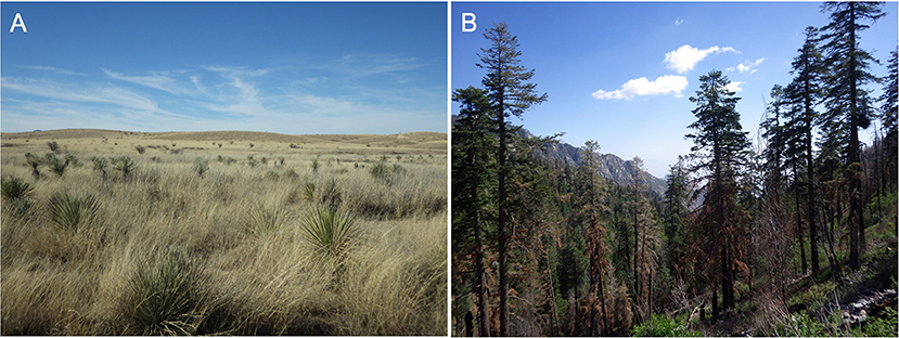
Figure 1. Landscapes vary in complexity. Panel (A) shows a southern Arizona grassland at Las Cienegas National Conservation Area, illustrating a landscape with low taxonomic diversity, plant functional trait diversity, and topographic complexity. Panel (B) by comparison, has higher complexity, with a clear legacy of disturbance by wildfire, high plant functional diversity and topographic complexity, and more interactions among a higher number of species. Photo from Mount Graham, in the Pinaleño Mountains of Arizona. Ecosystems and ecology are shaped dynamically by bottom-up factors such as local topography, spatial clustering of resources, and stochastic events such as ignitions, as well as top-down processes and controls such as temperature, precipitation, and other climatic factors. Disturbances such as wildfire and insect outbreaks are influenced by these factors and others, including phylogenetic history of organisms and their disturbance adaptations, physical structure and demography of organisms, and landscape history. However, knowing all of this information perfectly is not sufficient to predict fire behavior, initial ignition points, or extent of insect-caused mortality, because the features of emergent phenomena (such as disturbance regimes) are highly sensitive to initial conditions and may not be deterministic. Photo credits: E.A. Newman.

Although “complex” and “complicated” are often used interchangeably in the vernacular, complex systems have a number of important properties that go beyond mere complication. Various definitions for complexity have been proposed in different contexts (Kolmogorov, 1963; Gell-Mann and Lloyd, 1996; Bialek et al., 2001; Ladyman et al., 2013), but in general, more complex systems require more information to describe any given state of that system (Table 1 defines and explains bolded terms). Models of a complex system may also be complex (Kolmogorov, 1963; Edmonds, 2000), or have simple rules generating complexity, as in the case of fractals; and model complexity is sometimes used as an overall measure of relative complexity. In these ways, complexity and information theory (Shannon, 1948) are fundamentally linked. Complexity is sometimes associated with the physical entropy, rather than information entropy of a system (Figure 2), and quantitative relationships between complexity and both types of entropy have been proposed (Wolpert, 2013).

TABLE 1

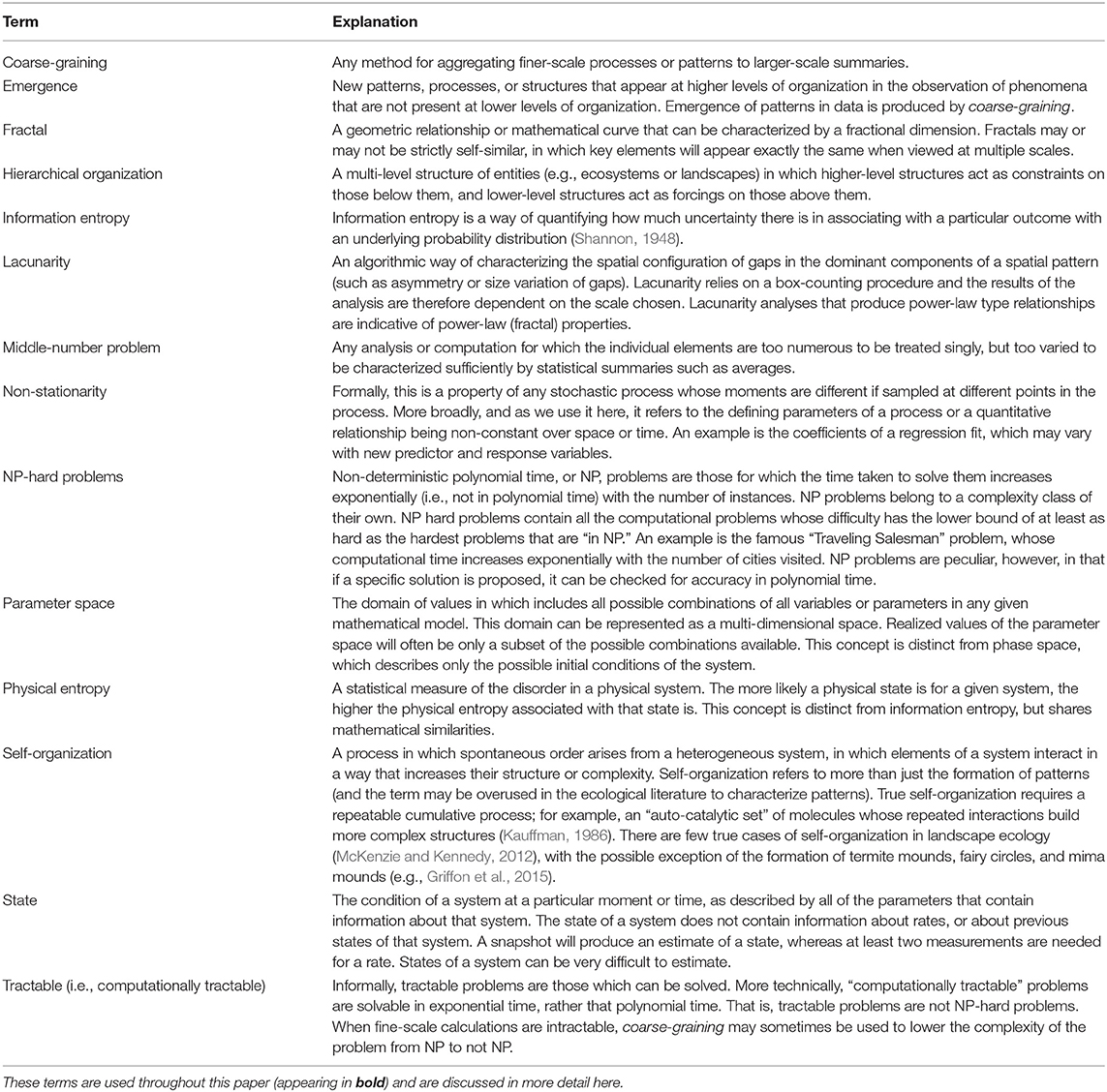
Table 1. Common terms in complexity science, as related to landscape complexity.

FIGURE 2

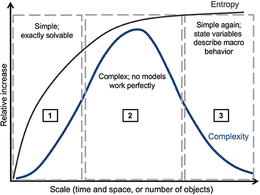
Figure 2. Schematic relationship between entropy and complexity. Entropy increases monotonically with increasing scales of physical systems, whereas complexity increases from (1) the region of fundamental physical models, (2) to the “middle-number domain,” but then decreases (3) as large systems are described adequately by aggregate properties. In region (1), models are deterministic and exactly solvable. In region (2), complex behavior of the system is controlled by interacting top-down and bottom-up processes, and models therefore will not provide perfect predictions of data. In region (3), statistics are highly aggregated for large numbers of interacting elements, and general laws emerge (for example, the Ideal Gas Law, the species area relationship in macroecology, or annual wildfire burned area at subcontinental scales).

As landscape ecology continues to develop as a field, it will be productive to engage the knowledge and terminology that have been developed in complexity science to define avenues of progress. In this paper, we approach landscapes as complex systems, and give examples of phenomena associated with landscape-level complexity that are challenges to defining models that cross scales of patterns and processes. We do not address complexity per se, which is itself a subject of much theoretical work (see Gell-Mann and Lloyd, 1996). Instead, we focus on three features of complexity that are intrinsic limitations, or challenges, to progress in landscape ecology. These features are: (1) coarse-graining, or how to optimally aggregate fine-scale processes to larger scales in a robust manner that minimizes error (Levitt and Warshel, 1975; Turner et al., 1989; Gorban, 2006); (2) the middle-number problem, which affects systems with enough elements to be computationally intractable, but with elements that are too few or too varied to be amenable to global averaging (Weinberg, 1975; O'Neill et al., 1986; Kay and Schneider, 1995; McKenzie et al., 2011a); and (3) non-stationarity, which refers to relationships or parameter choices that are valid in one environment in one domain (such as species distribution models), that no longer hold when projected onto other environments (Cooper et al., 2014), such as future scenarios of altered climate (Turco et al., 2018; Yates et al., 2018). Even with expected ongoing improvements in modeling, data collection, and data processing, these limitations are less tractable than other types of ecological modeling problems, such as missing data or variables. These limitations therefore represent underlying conceptual challenges in the field of landscape ecology. We describe different conceptual approaches that have been applied to modeling of scaling and complexity for landscapes, review their limitations and potential, and suggest potentially fruitful directions for future research in landscape ecology.

Phenomena Associated With Complex Landscapes

The study of landscapes, disturbance processes and disturbance regimes, and anthropogenic forcing of climate change occupies a domain in parameter space in which phenomena and the models that describe them become “complex” (Kolmogorov, 1963; Edmonds, 2000). When a system is described as “complex,” it means that observed phenomena are intrinsically difficult to model due to the dependencies or interactions between their parts (which has been referred to as “bottom-up” control on outcomes and system variables) or between a given system and its environment (also known as “top-down” controls on relationships among outcomes and system variables) (Reuter et al., 2010). Complex systems such as landscapes or general ecological systems have characteristics such as non-linearity, scale dependence, and emergence that make physical and ecological phenomena difficult to parse into independent variables, and prevent easy transference across space or time, or to different physical scales (Wiens, 1989; Yates et al., 2018). Simplifying assumptions about complex systems, such as not accounting for basic physical constraints (e.g., mass balance) in food web models, or modeling ecosystems as closed systems will lead to unrealistic results (Loreau and Holt, 2004).

In a complex system, emergent dynamics are not explained completely by simple reducible components, future states of the system may be deterministic and chaotic, or may contain stochastic components, and causal mechanisms are challenging to identify because any given component can act as both a driver and a response due to feedback mechanisms. Furthermore, the issue of prediction in complex systems poses a major challenge, because many future outcomes are possible, and these systems have high sensitivity to initial states of the system. The global climate system is a well-known example of a complex system with these properties. Because outcomes will be sensitive to initial conditions and may not be entirely deterministic, predictions about emergent behavior will never be perfectly accurate, even with increasing amounts of data and better computational resources (e.g., Lorenz, 1963; Figure 2). However, despite these limitations, reliable predictions are possible over short time horizons and for well-delimited questions where appropriate empirical data are available.

Landscape ecology, and particularly issues related to wildfire (a major focus of this manuscript), exemplifies many of these properties of complex systems. For example, in landscape fire, we often study the interplay and feedbacks between large-scale, top-down drivers of wildfire, such as climate and human land-use (Gill and Taylor, 2009), and more mechanistic and smaller-scale bottom-up drivers, such as ignitions, fuel patterns, and local topography (Falk et al., 2011; McKenzie et al., 2011b; Parks et al., 2012). Landscape ecology seeks to describe the dynamic relationships between ecological patterns and processes across spatial scales, from plot or forest-stand level to watersheds, from local regions to ecosections, or globally. Properties common to all complex systems, including self-organization, non-linearity, feedbacks, and robustness (including lack of central control) are reviewed in Ladyman et al. (2013) and elsewhere (Reuter et al., 2010). In studying the landscape ecology of wildfire, complexity is particularly expressed as emergence (section Emergence), landscape memory (section Landscape Memory), landscape resistance (section Landscape Resistance), and contagion (section Contagion). As a consequence, landscape fire ecologists inevitably confront modeling complexity, and must grapple with these problems through choice of variables, scale, and delimitation of a system that lacks closed boundaries.

Emergence

Emergence refers to new patterns, processes, or structures that appear at higher levels of organization in the observation of phenomena that are not present at lower levels of organization. Emergent phenomena are the products of causal mechanisms at lower levels of organization, but they are expressed primarily in behavior of high-order components. For example, many individual mechanical parts of a watch, when organized correctly, can track time together, but the individual parts cannot do this by themselves. Similarly, the functioning of social insect colonies results from the actions of individual worker insects with different tasks, and vehicle traffic patterns are the emergent result of individual drivers' choices about travel. The property of life in organisms is itself an emergent property of the organization of molecules and biochemical pathways. Emergent processes must be consistent with finer-scale laws and cannot violate them; for example, biological processes have independent dynamics not fully explained by the laws of physics, but they are nonetheless subject to them.

Many phenomena of landscapes result from emergence, including community-level structure and function, disturbance regimes, physiognomy of vegetation (forested landscapes vs. savannas, for example) and patch formation and dynamics (White and Pickett, 1985; Wu and Loucks, 1995; Bormann and Likens, 2012). Landscape patch patterns are often a legacy of many disturbance events (Cuddington, 2011; Figure 3). Landscape patches are identifiably distinct areas of any size in the spatial pattern of a landscape, such as the mosaic of burned and unburned areas in a large landscape wildfire. Burn-severity patches are the emergent result of the landscape distribution of fuels and fuel conditions, individual plant susceptibility to heat damage to living tissues, topographic influences on fire spread, fine-scale patterns of wind, and combustion physics at the submeter scale. The size distribution and spatial structure of the post-fire patches are primary drivers of finer-scale landscape-ecological processes such as tree regeneration, which is constrained by seed availability and suitable recruitment environment, and future fire spread, which can either be constrained or accelerated by fuel availability (Collins et al., 2017; Davis et al., 2019). Such outcomes have led to the ideas of downward causation (Campbell, 1974), in which processes at lower levels (here regeneration and fire spread) appear to be responding to emergent forcings, and contextual emergence (Atmanspacher and beim Graben, 2009), or how contingencies at more complex, higher levels of description provide the “context” for outcomes at lower levels (Flack, 2017).

FIGURE 3

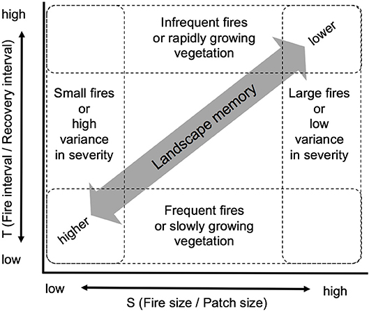
Figure 3. Relationships between landscape memory and scales of time (T) and space (S) of landscape disturbances. The “landscape memory” of a disturbance decreases as the ratio of disturbance interval to recovery interval increases, and the ratio of disturbance size to patch size of the affected landscape increases. Revised, with permission, from McKenzie et al. (2011b).

Landscape Memory

Landscape memory or ecological memory, is a generic term for the legacies of landscape process and pattern, including their longevity and the strength of their influence on current landscape dynamics (Peterson, 2002; Turner, 2005; Johnstone et al., 2016). It also includes concepts of legacy effects of prior disturbances and use of the landscape (Cuddington, 2011). Johnstone et al. (2016) decompose ecological memory into two forms of legacies: informational, which derives from species life-history traits and adaptive potential; and material, which encompasses physical legacies such as soil and seed banks. In the context of fire regimes, landscape memory can be short-lived and “ephemeral”; or long-lived and “persistent,” depending on the frequency and severity of disturbances (van Mantgem et al., 2018). A grassland with frequent fire and rapid regrowth may have a relatively short-term landscape memory for any particular fire event, whereas the legacy of wildfire in a forest with long-lived tree species may persist for multiple centuries (Figure 3). McKenzie et al. (2011b) propose a spatio-temporal domain of landscape memory as a function of scalable elements of fire regimes (section Energy and Regulation Across Scales).

In wildland fire, the legacy of individual fire events and the properties of the dominant plant community form a dynamic system in space and time. For example, the behavior of a wildfire (rate of spread, flame length, heat output per unit area and time) is conditioned at each moment of combustion by multiple properties of topography (slope, aspect, topographic position), weather (wind direction, air temperature and humidity, precipitation, ignition sources such as lightning), and vegetation (woody and herbaceous biomass, three-dimensional spatial distribution, water content of live and dead fuels). Fire behavior interacts with species' life-history traits and effects on soils to constrain individual survivorship and mortality, the primary metrics of fire severity (Keeley, 2009). Plant condition and prior fire exposure also influences post-fire mortality (van Mantgem et al., 2013, 2018).

The behavior and effects of wildfire then set the stage for post-fire ecological and hydrologic processes. Soil stability and permeability strongly regulate the speed with which vegetation can become re-established; severely burned hydrophobic soils take longer to become plant-suitable, and some plant guilds may be excluded initially by soil properties alone. The landscape mosaic of burn-severity patches and residual vegetation governs the post-fire trajectory, especially in large (>10³ ha) patches with few or no surviving trees. These areas must be recolonized by dispersing seeds from relict tree islands or adjacent surviving trees, which is a strongly scale-regulated process because the effective seed dispersal radius of many species is 250 m or less, and successful seedling establishment can be limited by the availability of safe sites and suitable climate (Stevens-Rumann and Morgan, 2016; Davis et al., 2019; Law et al., 2019). Recolonization of large high-severity patches can take decades or even centuries, leaving a persistent legacy of plant age classes, forest physiognomy, and species distributions that create the conditions that will regulate the next fire event (Collins et al., 2009, 2017).

Landscape Resistance

Landscape resistance is a spatially structured characteristic of landscapes, quantifying resistance to movement with respect to a particular agent or process. Typically, this concept is applied to animal movement (Keeley et al., 2016), but it can also be applied to disturbances. In the former, it is often a function of variation in habitat suitability or topography; with fire, it is a function of barriers or pathways to fire spread, such as steep topography or rivers and other non-flammable elements. Landscape resistance controls the optimal paths of fire spread and the minimum travel time of a disturbance between locations, primarily through the influence of topography and fuels over landscape space (Finney, 2002). For example, Conver et al. (2018) mapped the most parsimonious fire spread pathways in a forest-grassland ecotone in northern New Mexico, and showed that fire followed pathways of optimal fuel mass, moisture, and tree cover, reflecting the physics of a spreading fire. The inverse of resistance is connectivity, which is a combined effect of various landscape properties that facilitates the flow of mass or energy, and is related to contagion. Resistance (connectivity) is an emergent landscape property resulting from the condition and spatial distribution of large number of individual plants, as well as their associated soils and topographic position.

Contagion

Contagion is a property of disturbances that propagate within a conducive medium. Contagion requires two elements: connectivity and inertia (or “momentum”). Connectivity allows the spread of a disturbance from one part of the medium to another, whereas inertia represents the ability of the disturbance to overcome some threshold and be passed from one unit to another. Without enough inertia or momentum, the contagion will eventually end; but with enough momentum, a contagious disturbance will “percolate” and affect the majority of the elements of the community (Balcan and Vespignani, 2011). Contagion is sometimes modeled as connectivity of networks, with the nodes in a network representing actors in the network, and edges representing the connections between them as the specific interaction being modeled. Nodes may be species, individuals, or locations; edges may represent disease or bark beetle outbreaks. For example, infectious disease, such as root rot in trees, is a contagious disturbance that be modeled as an interaction network (Delmas et al., 2019). The two nodes representing hosts or potential hosts of the disease would have one edge between them, representing an interaction of passing an infectious agent, if one party has infected another. Inertia in this case may represent the disease having to overcome a host's immune response. Networks may also be modeled with latency, to mimic dynamics and time-dependence of infection and spread.

Contagion can alternately be modeled without the network paradigm (Peterson, 2002). For example, wildfire spreads through the medium of flammable vegetation and must cross the threshold of ignition temperatures to initiate fuel pre-heating and pyrolysis, which ultimately set up the chain reaction that allows fire to spread from one flammable element to another in space and time. Similarly, insect outbreaks propagate through vulnerable host species of the correct age or size, overcoming the defensive mechanisms of trees to make use of the individual tree. In these cases, contagion is often modeled as a function of proximity of one grid cell, representing either an area or an agent, to another. Such disturbances are “contagious” disturbances, whereas hurricanes, tornadoes, and other storms are not.

With wildfire, both contagion and landscape resistance are relevant primarily within at medium spatial and temporal scales that have high complexity (region 2 in Figure 2), ranging from submeter scales to tens of kilometers. For example, models of fire spread at the degree or half-degree grid spacing of global climate models are extrapolated outside the domain of contagion, as the spatial variation that controls fire spread is much more finely scaled (McKenzie et al., 2014) and the physical process of spread, coarse-grained to that level, is unrealistic compared to fine-scale physical models of combustion (Parsons et al., 2017). This middle domain of spatial scales has the greatest complexity (section The Middle-Number Problem).

Challenges to Progress in Modeling Complex Landscapes

Coarse-Graining

Coarse-graining refers to processes in both the real world and in scientific methodology, that is, both physical and statistical processes. In both cases, coarse-graining is defined as the way in which processes, structures, and states aggregate and are combined into fewer larger entities to reduce modeling complexity (Levitt and Warshel, 1975; Gorban, 2006). In the physical world, coarse-graining produces emergence (section Landscape Resistance), as physical systems combine progressively, for example, from atoms, into molecular, chemical, biological, and then ecological systems. At each level, processes and patterns are observable that cannot necessarily be inferred from those below or above. Classic examples in the physical world includes the coarse-graining of statistical mechanics to classical thermodynamics (Jaynes, 1957), and the development of global-scale climate dynamic general circulation models (Meehl, 1990). In ecology, classic examples are the coarse-graining of individuals to populations, species to communities, and the combination of biological organisms interacting with abiotic conditions to well-defined ecosystems. In ecological modeling specifically, we aggregate discrete processes like predation to population cycles, sub-daily processes like photosynthesis to annual productivity, and fine-scale processes such as fire and bark-beetle behavior to landscape modeling of disturbance. This results in the emergence of aggregate patterns (of patch sizes, for example; Povak et al., 2018), that are scale specific (Figure 4).

FIGURE 4

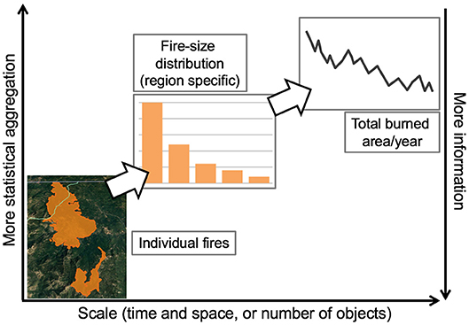
Figure 4. Coarse-graining leads to useful metrics at the largest scales, but reduces the amount of event-specific information retained in each step of statistical aggregation. In this schematic example, coarse-graining applies to individual fires, where information such as location, perimeter, point of ignition, severity, topography, local temperatures, and other information are known. One first step of coarse-graining produces a fire-size distribution, where information on number of fires and area burned are known for some time period. At this level of coarse-graining, trends in aggregate properties of multiple fires are detectable, but still scale-dependent. A fire-size distribution emerges from a second step in coarse-graining, which maintains information about area burned for comparison over large time scales or large regions, but loses information about number of fires. The observed pattern in this second step will also depend on the spatial extent of the data. Other forms of coarse-graining, such as those employed in macroecology, will result in other emergent properties, some of which may be independent of scale.

Many coarse-graining methods in the physical sciences draw on the availability of state variables at fine and coarse scales, i.e., microstates and macrostates. For these cases, coarse-graining has been termed “state-space compression” (Wolpert et al., 2017) and produces canonical algorithms to optimize its accuracy and minimize computational costs. Wolpert et al. (2017) provide a roadmap for this (Figure 5), which we draw on below.

FIGURE 5

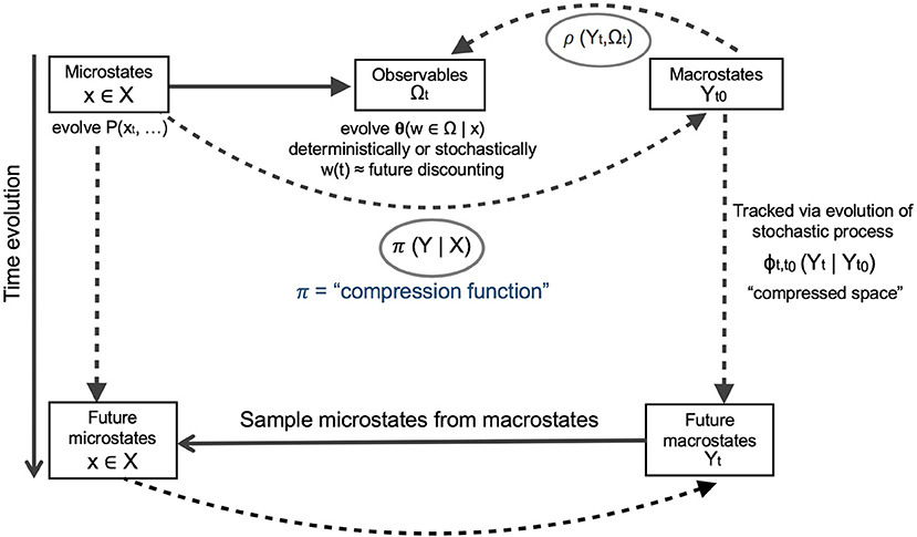
Figure 5. A roadmap for a rigorous approach to coarse-graining in complex systems, from Wolpert et al. (2017). The key to optimized coarse-graining is a “compression function,” here designated as π(Y|X), which translates microstates (fine-scale information X) into macrostates (broad-scale or “landscape scale” information Y). To ensure that the choice of compression function is optimal, we model the time evolution of the macrostates identified by π(Y|X) in parallel with evolution of the original microstates. Some combination of π(Y|X), the computed macrostates of the system “Y,” the time evolution of macrostates by a stochastic process φ, and the mapping of macrostates onto observables by some empirical relationship ρ will be optimized by a multivariate objective function. Our focus here is on π(Y|X), to address the coarse-graining challenge, for which some choices include simple adding up, regression, simulation, and maximization of information entropy.

Building models to analyze data requires two forms of scaling: choosing the grain size of the data, which is the coarse-graining procedure, and then choosing an extent that the data represent. Grain and extent are two primary properties of scale (Turner et al., 1989; Palmer and White, 1994; Wu, 2004). Models of a process or structure are usually specified at a scale that is optimal, or at least convenient, for analysis that is informative and tractable to solve a particular problem (Levin, 1992). For example, in GIS work, units of data may be observations and climatic variables may be aggregated to a grain size of 1 km², and analyzed across an extent of a watershed, or some other landscape unit where the extent is much larger than the grain size. As noted by Turner et al. (1989), tracking the loss of information with changes in grain size and extent of data explicitly may be key to predicting and correcting for that lost information. Investigating scaling relationships in this manner may make it possible to correct for statistical biases introduced by coarse-graining.

We can aggregate measurements of finer-scale processes and models to summarize measures of central tendency and higher moments (such as variance) of their distribution. We may also need to transform variables qualitatively while trying to minimize error propagation across scales. With fire, for example, heat transfer in physics-based models at sub-meter scale (Mell et al., 2007) becomes fireline intensity at the fire front at the meter scale, producing fire spread that depends on external kinetic energy, such as from wind and solar heating, and landscape connectivity at the scale of tens to hundreds of meters. At even coarser scales in space and time, we reach annual area burned, fire size distributions, and fire regimes, whose nature and complexity are the domain of landscape ecology.

In this sense, coarse-graining is a method that is used to reduce modeling complexity by side-stepping the middle-number problem, but the use of coarse-graining poses its own challenges. In complex systems, coarse-graining is never a perfect solution to the middle-number problem, because, as demonstrated by Essex et al. (2007), “systematic modeling errors might survive averaging over an ensemble of initial conditions,” which can lead to the introduction of an unknown amount of bias into any prediction, and to unpredictable “surprises.” These surprises might consist of sudden state shifts (in the climate system, for example) due to undetected internal dynamics. However, in the case of mechanistic models using coarse-grained variables, predictions that can be validated over short time horizons or when models using these variables are transferred to similar environments can also be used to judge the validity of that model (Houlahan et al., 2017) (though the same may not be true of entropy-based models; see Dewar, 2009).

With particular relevance to landscape ecology, challenges imposed by coarse-graining include:

• Loss of important information. Physics is realized at sub-millimeter to meter scales, and the processes of interest are often non-linear rather than additive. In fire behavior, this is a large source of uncertainty (Mell et al., 2007).

• Regression to the mean removes information about heterogeneity, and may introduce statistical bias (Essex et al., 2007). We lose measures of variability, and estimates of the mean, variance, and higher moments of the distributions of random variables being measured. This is a particularly difficult source of error when there is spatial or temporal autocovariance (Kennedy and Prichard, 2017).

• Underrepresenting the influence of extreme events, because aggregating controls variability (see Levin, 1992 on the relationship between variance and window size). More technically, because we are often forced to implement coarse-grained processes stochastically, we can arrive at arbitrary realizations that are difficult to validate against observations (Lertzman and Fall, 1998; Deser et al., 2012).

The Middle-Number Problem

The middle-number problem refers to the domain of data complexity in which neither local mechanistic models nor generalized global relationships holds exactly, although both local and global processes exert influence on observed patterns. As we move from small numbers of objects or events (e.g., local datasets) to larger numbers (e.g., regional or global datasets), we cross a zone of complexity known as the “middle-number domain” (Figure 2). In this domain, systems contain enough elements to be computationally intractable, but too few elements, or elements that are too heterogeneous, to be amenable to global averaging (Weaver, 1948; O'Neill et al., 1986). The basic problem of predicting species richness in a local region from larger averages falls into this category, as richness may be known at the ecosystem scale, but controlled by a huge variety of factors at smaller scales, ranging from moisture availability and soil type, to the presence of predators or pollution. Similarly, weather is famously hard to predict in the long term, because of the small-scale factors that influence it (Lorenz, 1963).

In the middle-number domain, fundamental physical models that apply at fine scales are no longer adequate because the systems are driven by both “lower-order” (mechanistic and physical) and “higher-order” (context) processes. These medium-scale processes and heterogeneity prevent global models from making completely accurate predictions over subsets of their domains. This region is one in which self-organization occurs, in which elements of a system interact in a way that increases their structure or complexity, sometimes resulting in pattern formation. Predictions about future states of a system, or relationships between elements, are computationally intractable in this region, in the sense that they may correspond to what are known in computational complexity theory as NP-hard (Non-deterministic Polynomial-time) problems (Papadimitriou, 2003).

A classic example of the middle number domain in physics is “in between” statistical mechanics descriptions of individual molecular motion, and classical thermodynamics, which characterizes systems by their pressure, volume, and temperature, which are averages of the properties of large numbers of particles in motion. In ecological systems, individual organisms are the analog of molecules and are described by individual interactions and physiology models, whereas regions or continents of ecosystems are the analog of aggregate thermodynamics, and are well-described, for example, by macroecology (section Macroecology). In between, on the landscape, or watershed, there are too many elements to constrain individually, but not enough (with manageable heterogeneity and variance) to model with high precision in the aggregate.

Simplifying assumptions may reduce computational complexity, but these assumptions can backfire. Even with the best possible information, uncertainty and bias can survive averaging and aggregation through long-term forecasting (a modeling error that it may or may not be possible to detect), leading to unpredictable state changes (Essex et al., 2007). In a fascinating report that takes on complexity issues in ecological prediction without a specific system, Cooper et al. (2014) show that excluded variables and interactions (or small perturbations within the training region) can lead to arbitrarily large forecasting errors in complex systems outside the training domain. This reinforces how important the selection of appropriate models is, and in the case of mechanistic models, correct predictions provide a necessary form of validation (Houlahan et al., 2017). This logic can be extended to better understand which environments are suitable for model transfer, rather than approaching the question from the side of which model may best be used for all environments and time periods.

In landscape fire, we extend the ideas of McKenzie et al. (2011a), from the scale at which the middle-number domain begins (i.e., smallest spatial scale or smallest number of interacting elements), to scales at which explicitly spatial interactions become both numerous and relevant. For example, post-fire recovery is dependent on the interactions among the individual-level processes of survivorship, reproduction, and growth, and the equivalent interactions of competition, mutualism, and dispersal. These individual-level processes aggregate to produce the legacy of past fires, watershed-scale topography, and the weather associated with the subject fire. Analogously, the middle-number domain ends (largest spatial scale) where connectivity, or contagion, and landscape resistance cease to be important proximate controls on fire-scale processes. For instance, our understanding of fire regimes at the scale of ecosections (variable in size but at least 100s of square kilometers) comes in terms of area burned and top-down climatic regulation (e.g., Parisien and Moritz, 2009; Moritz et al., 2011; Littell et al., 2018), which unlike fuel models, is no longer dependent on the characteristics of individual organisms. We can predict fire regimes (emergent properties of multiple events in space and time) at the scale of ecosections, and fire behavior at scales of centimeters to tens of meters, but when we try to follow how fires initiate and spreads contagiously over large landscapes, we have a coarse-graining problem, and a middle-number problem, up to the limit of the extents of the largest fires. In theory, an error-free coarse-graining would resolve the middle-number problem for its specific case, but error propagation with increasing scale and level of organization is an inherent challenge.

In summary, with reference to landscape ecology, the middle-number problem can be characterized as the following:

• Outcomes are sensitive to many variables, each of which is distributed non-uniformly in both time and space.

• The relative importance of variables (drivers) changes with scale. Lower- and higher-level processes change in both strength and heterogeneity with the scale being examined.

• We observe and measure what is emergent (observations are the results of these interactions), but we may not witness the process of the interactions themselves. More specifically, we cannot compute the outcomes of fine-scale mechanisms at large scales and temporal extents without simplifying assumptions.

• Important outcomes, including those most relevant for management and policy, are often desired within the parameter space in which complexity is greatest, and where variation occurs at multiple scales.

• Projections of models from one region of training (one part of the middle-number domain) to another can lead to unbounded, or arbitrarily large errors (Cooper et al., 2014).

Non-stationarity

Non-stationarity refers to the limitations of using models with adjustable parameters to predict future states (Wolkovich et al., 2014; McKenzie and Littell, 2017; Turco et al., 2018). These include most empirical statistical models and many “process-based” models: those that use mathematical relationships involving parameters that have been estimated from data, even when the model is said to represent a physical or biological mechanism. In time series and spatial statistics, stationarity is the property that the generating function for a stochastic process is constant. This means that the underlying probability distribution of an observable (a physical quantity that can be measured), typically its mean or variance but also including its autocorrelation function, is not spatially or temporally dependent. When we model relationships using empirical data from current and past observations, we estimate a particular distribution (mean model and variance/covariance matrix) from a discrete environmental domain, such as the relationship of tree growth to soil moisture or the relationship of soil respiration rates to temperature. When these empirical models are used to project into the future, it is implicitly assumed that the distributions are stationary. That is, the mean value (or model, and associated variance/covariance matrix) we estimate currently for the relationship among variables, e.g., a regression coefficient, will be the same mean value (or model) in the future, or in a different place.

In the context of landscape fire, stationarity is often implied with use of the historical range of variation (HRV) in fire regimes (Morgan et al., 1994; Keane et al., 2009). Stationarity in the HRV sense implies stability over space and time in the statistical distribution of a variable (such as fire frequency or fire-size distribution), including central tendency, but each of these variables may exceed its historical distribution when the underlying drivers go outside their historical range (Elith and Leathwick, 2009). A more robust definition of stationarity is stability in relationships among variables, even when a driving variable exceeds its historical range; for example, the relationship between maximum annual temperature and annual area burned at large scales. In the context of current and projected environmental change, the best practice in statistical models is to make predictions only within the domain of the data used to estimate the model; where the driver is projected to fall outside the historical envelope, statistical models may be unreliable (McKenzie and Littell, 2017; Turco et al., 2018). In that case, other types of models, such as purely mechanistic models, or models that rely on the functional traits of organisms (Dobrowski et al., 2011; McDowell and Allen, 2015) must be employed.

By definition, we cannot expect stationarity to hold uniformly in the context of current and near-future climate change, where the distributions of climatic drivers of ecological dynamics are and will be departing from their historical means and ranges. For example, the strength and direction of the correlation between annual area burned and water-balance deficit varies across the western USA, depending on the distribution of the water deficit (McKenzie and Littell, 2017; Littell et al., 2018). In ecophysiology, the strength of climate-growth relationships of trees (e.g., the correlation between annual increment and precipitation) varies over time and broader climatic cycles, also depending on the distribution of the climatic driver (Marcinkowski et al., 2015). In both these cases, the adjustable parameters, or specifically the regression coefficients in a statistical model, vary over the spatial domain of the data, and will certainly also vary over time in a non-constant climate.

In summary, with reference to landscape ecology, the non-stationarity problem is that:

• Most mathematical relationships used in models include adjustable parameters.

• In empirical studies, these parameters, and the relationships between the parameters, change across both space and time (Dobrowski et al., 2011).

• Projections for the future that rely on models fit from observations therefore are fragile to expected changes in these parameters (Yates et al., 2018).

• Important examples for fire, relevant to management and policy, are statistical relationships between climatic drivers and fire effects at the level of individual organisms and associated soils, with implications for aggregate properties such as annual area burned (Littell et al., 2018), fire-size distributions (Reed and McKelvey, 2002), occurrence of extreme events (Stavros et al., 2014), and spatial patterns of fire severity (Cansler and McKenzie, 2014).

Interactions Among These Challenges

These challenges do not arise in isolation; interactions among them will confound proposed solutions to one or more of the challenges. For example, it has been argued that fully mechanistic models should be a goal in landscape simulations because they optimize adjustable parameters to be most able to be projected into new environments (Keane et al., 2015). In theory, fully mechanistic models avoid the non-stationarity problem because the model will be perfectly transferable as long as it includes all the mechanisms that affect the observables (see Gustafson, 2013 for a landscape modeling example). There are two problems with this claim: first, many so-called “mechanistic” mathematical models include parameters that are fitted from data that do not sample the full range of conditions and therefore cannot determine exact mechanisms. Second and perhaps more importantly, extrapolating fine-scale computations (which mechanistic models invariably are, e.g., physics-based fire models) to larger scales of interest runs into the middle-number problem. Computations become intractable (because they are NP-hard; for a useful discussion of this topic relevant to biology; see Felsenstein, 2004), and the demands of data and associated data input uncertainty increase (Kennedy and McKenzie, 2017). A solution to this middle-number problem therefore may lie in coarse-graining both model processes and associated input data in a way that minimizes error, but this encounters problems imposed by non-stationarity. In this sense, solving the middle number problem may be possible only in stationary systems; solving problems in non-stationary systems will require inventive applications of coarse-graining to avoid the middle-number problem. In landscape ecology, joint solutions to these challenges are uncharted territory. Below, we describe some potential paths to solutions that have particular relevance to cross-scale analysis of landscapes as complex systems.

Approaches to Understanding Complex Landscape Phenomena Across Scales

Models in landscape ecology that work well across scales, solving the above challenges, will involve quantitative scaling laws that combine top-down and bottom-up perspectives. Multiple disciplines, such as physics, biology, and ecology, have incorporated quantitative scaling relationships in an attempt to model phenomena that cross physical scales. In landscape ecology, the following concepts and paradigms show promise for solving the coarse-graining, middle-number, and non-stationarity problems. The first, Hierarchical Patch Dynamics, involves hierarchical organization applied to discrete spatial scales thought to be most important, whereas the next three (lacunarity, Energy and Regulation across Scales, and Macroecology) invoke quantitative scaling laws that are or are nearly continuous in large systems.

Hierarchical Patch Dynamics

Hierarchical Patch Dynamics (HPD) is a proposed paradigm shift, or new framework, for ecology, espoused by Wu and Loucks (1995). Its goal is to resolve problems of scale and non-equilibrium in ecological systems. This idea is similar to contextual emergence, in the sense that the framework contains levels of complexity, in which larger scales are more complex than the smaller scale items that they contain. In HPD, patches of ecosystems interact at multiple scales, and hierarchy theory provides a means for quantifying and ordering phenomena at multiple scales.

The major elements of HPD (Wu and Loucks, 1995) are that (1) Ecological systems can be modeled as nested discontinuous hierarchies of patch mosaics (see also Holling, 1992). Patches are structural and functional units, and they are nested, meaning larger patches contain smaller ones. A defining assumption is that patches can be nested perfectly, and that the highest level of organization is not contained by any of the smaller ones. (2) System dynamics are a composite of patch dynamics. This simplifying assumption states that individual patch changes can be aggregated meaningfully such that overall system dynamics are recoverable from their composite. (3) The pattern-process scale perspective. This restates the landscape ecology paradigm that pattern and process interact mutually and recursively at multiple scales. (4) Non-equilibrium. Transient dynamics can dominate at small scales, but this leads to: (5) Incorporation and metastability. With the etymological meaning of “incorporate,” fine-scale transient dynamics are literally swallowed up by stabilizing forces at “meta” scales (implying the middle-number domain), whereas at very broad scales stochastic processes dominate again. Note that this is opposite to our view of the middle-number problem and its domain as being the least stable, at least in the sense of predictability.

A limitation of this paradigm is that it assumes that coarse-graining is a straightforward outcome of aggregating the dynamics of nested patches. We have seen (section Landscape Resistance) that emergent properties at coarser scales are not necessarily direct outcomes of fine-scale dynamics, and that additive processes are only a subset of coarse-graining, whether observed or modeled (Wolpert et al., 2017). This conceptual framing does not directly map onto a unique way to aggregate, or coarse-grain the middle number domain. Although some problems of the middle number domain may be solved through this aggregation of patches (Wu and Loucks, 1995), the framework of HPD may simply not be mathematically rigorous enough to solve all problems associated with the middle number domain; indeed, not all such problems may be solvable. It is now known that uncertainty and bias can survive averaging and aggregation through long-term forecasting (a modeling error that it may or may not be possible to detect) (Essex et al., 2007), and that small perturbations or “unimportant” missing variables in a training region of a model can lead to predictions where there is no meaningful bound that can be placed on the error of the model outside of its original training data (Cooper et al., 2014). That said, HPD does offer an important framework for modeling discrete scales in landscape dynamics, especially in the context of non-equilibrium states.

To address our three challenges, HPD would, in theory, assume that discrete scales in space are metastable, extending upward through the middle-number domain. These scales are the domain of ecosystem dynamics, sensu Holling (1992). There is an implicit link to hierarchy theory (O'Neill et al., 1986), in which cross-scale dynamics are clearly defined and directional. This means that processes increasing in scale are driving, whereas processes decreasing in scale are constraining. In theory, this hierarchical structure entails the optimal degree of coarse-graining. Analogously, non-stationary dynamics are subsumed into the hierarchical patch structure.

Lacunarity

Lacunarity is way of characterizing the spatial configuration of points or other components of a spatial pattern, such as patches or pixels. The lacunarity algorithm is a “box counting” procedure that specifies a grain size over a region of interest, and quantifies the presence or absence of a phenomenon in each “box” (Allain and Cloitre, 1991). Specifically, lacunarity is a dimensionless metric that estimates the roughness of a pattern as a fractal dimension, and identifies gaps in the overall patterns (Plotnick et al., 1996). Highly heterogeneous patterns with low rotational and translational symmetry have high lacunarity (and high complexity), whereas mostly homogeneous patterns that have high rotational and translational similarity are considered to have low lacunarity (and low complexity; Karperien, 2013). With this metric, we can obtain a form of the variance-to-mean ratio that is calculable and directly comparable across scales. Lacunarity estimates may complement estimates of fractal dimension, but provide further information in that the shape of lacunarity curves (with increasing window size) can illustrate departures from a self-similar or isometric character at identifiable scales (Dale, 2000).

Lacunarity is a static property of patterns, and is generally used to quantify properties of self-similar fractal-like patterns to determine the fractal power that describes them. Lacunarity has been adopted in landscape ecology for data sets that are not necessarily self-similar, such as seedling counts along transects and other two-dimensional patterns, like landscape patches (Plotnick et al., 1993, 1996; Swetnam et al., 2015). In landscape ecology, lacunarity can be seen as an aggregate expression of processes, such as disturbance and competition, that create landscape memory. With respect to landscape fire, the lacunarity index at a broad scale is computed directly, and consistently, from spatial patterns of fuels and topography. This is demonstrated in Kennedy and McKenzie (2017), where lacunarity is used to compare simulated and observed patterns of fire spread in a forested landscape to evaluate a stochastic fire model whose objective is to replicate fire-regime properties, rather than individual fire perimeters. Lacunarity also captures scale automatically through the specification of a grain size and extent, which leads the way into investigations of spatial heterogeneity and spatial statistics in landscapes (Wagner and Fortin, 2005).

With reference to the three challenges we have posed, lacunarity collapses scale-specific metrics into one that is especially robust across scales, thereby using a form of coarse-graining with minimal error. In theory, this avoids the numerosity associated with the middle-number problem and the need for adjustable parameters. An obvious limitation of lacunarity is the reliance on one metric to capture what are often noncommensurate aspects of complexity, which are measured in different units (for example, landscape complexity associated with succession and demography is measured in different units than phylogenetic information). Whereas lacunarity can adequately represent an aggregate of processes, it is not possible to recover the ecological information lost in the aggregation process, and it would be difficult to track error propagation associated with this extreme level of coarse-graining.

Energy and Regulation Across Scales

Energy and Regulation across Scales (ERS) is a conceptual framework for understanding contagious disturbance on landscapes (McKenzie et al., 2011a), developed specifically for modeling landscape fire. ERS aims to identify scaling relationships that accomplish coarse-graining without some of its most error-prone components: (1) aggregating elements that have substantial uncertainty associated with them, and (2) changing variables across scales with ad hoc methods. ERS separates the important drivers of contagious disturbances on landscapes into their fundamental elements, Energy, and Regulation. With suitable metrics for each, they can be applied across both spatial and temporal Scales in a way that minimizes the coarse-graining errors associated with changes of variables.

Energy is the fundamental “currency” of wildland fire, in that it can be measured and tracked across scales with no change of variables. Although vegetation on a landscape is often described in terms of stored mass or carbon, the fundamental nature of wildfire reminds us that vegetation can also be described in terms of its embodied energy. All biomass consists of both atomic mass and molecular bond energy. The atomic constituents of photosynthesis and carbon fixation (C, H, O) are organized into more complex molecules with higher energy content. The bond energy in these more complex molecules thus reflects the net energy captured during photosynthesis and subsequent carbohydrate synthesis. Energy storage on the landscape scale is regulated by factors that govern net primary productivity (Rasmussen et al., 2011; O'Connor et al., 2017).

Energy can be measured and calculated in the same units (joules) at any scale. The cycling of kinetic and potential energy (sensu Figure 1.4, McKenzie et al., 2011a) subsumes the variety of ecological dynamics imputed to the “fire landscape,” including fire behavior, fire effects, and vegetation succession. These latter are fragile to changes in scales of measurement and modeling, and have different units. Energy can be represented by a scalar quantity, but in the landscape context it can be vectorized, for example, as a vector field of wind containing a certain amount of energy, that drives fire behavior.

Regulation is an umbrella concept representing constraints on kinetic energy, and may be represented as a scalar, vector, or even a tensor quantity. For example, humidity can be represented as a scalar quantity, and will regulate combustion and fire spread. Humidity could therefore be expressed theoretically in units of reduced kinetic energy of the system. Another type of regulation is anisotropic topographic complexity, made up of a scalar element, representing a magnitude, and a tensor element, incorporating direction and directional response to interactions. If regulation can be represented as a dimensionless and normalized scalar quantity, it could be robust to spatial scaling. As a vector or tensor, the directional component may be an additive quantity, scaling linearly with area. A scalable representation of regulation in ERS will produce landscape resistance, or reduce contagion. Its spatial variation will produce lacunarity. Ideally, these complex attributes of the middle-number domain can be realized with minimal error propagation across scales.

As proposed, two problems need to be solved in order to implement an ERS framework. First, Energy and Regulation need to be reconciled in a way that is computationally tractable by appropriate choices of the scales at which their interactions are calculated. The scaling laws that we seek will be “grounded” at regions in scale space at which there is the most “action” (sensu Holling, 1992). For example, in complex topography, the obvious scales of variation of kinetic energy (e.g., wind), potential energy (e.g., fuels for fire or hosts for insects), and the two types of regulation will all be different. Second, the mathematical representation of coarse-graining of some aspects of regulation (e.g., topographic complexity) remains to be articulated so as to avoid a middle-number problem (e.g., being overwhelmed by numerosity).

ERS would, in theory, address all three of the fundamental scaling challenges by (1) adoption of the two canonical variables, Energy and Regulation, and (2) estimating the shape of universal scaling laws, as in macroecology (Wilber et al., 2015) by explicitly taking into account the scale of the processes under consideration. Whether these scaling laws would be “stationary” has not yet been addressed. It is likely that ERS would need a “meta-stationary” framework to approximate complex landscapes, where in the aggregate, landscapes would have approximately stationary, non-ergodic realms that produce aggregate patterns.

Macroecology

Macroecology is a subdiscipline of ecology that seeks to find and be able to predict universal patterns and explicit scaling laws in systems that are organized across multiple orders of magnitude of space and time. Brown (1999) characterized macroecology as “an approach to studying a certain class of complex ecological systems” and “as a way of investigating the empirical patterns and mechanistic processes by which the particulate components of complex ecological systems generate emergent structures and dynamics.” Macroecologists have long sought to explain and predict patterns of biodiversity, including species richness over area, abundances of species, and allometric scaling relationships (West et al., 1997; Enquist et al., 1998; Niklas and Enquist, 2001). By investigating patterns explicitly while controlling for the effect of scale, macroecology becomes a form of statistical aggregation that is a method of coarse-graining (Maurer, 2005; Storch et al., 2008; Bertram et al., 2019). For patterns in ecosystems that consider organisms and their physical characteristics, diversity, and spatial distribution, macroecology may offer the most reliable coarse-graining approach, in that it side-steps the middle number problem (Figure 2) by not trying to model mechanisms that lead to pattern formation at all scales; focusing instead on aggregate properties of large numbers of elements. Often in ecology, these elements are individuals, populations, or species. This idea of macroecology as a meaningful form of statistical aggregation is consistent with McGill's proposed definition for macroecology (McGill, 2019): “the study at the aggregate level of aggregate ecological entities made up of large numbers of particles for the purposes of pursuing generality.”

In attempting to characterize universal ecological patterns, such as the species area relationship, the species abundance distribution, and various metabolic relationships, some modern forms of macroecology embrace the complex nature of information underlying these patterns, and their predictions are based on maximizing the information entropy of the system. Information entropy is a way of quantifying the uncertainty associated with a particular outcome drawn from an underlying probability distribution (Shannon, 1948). Maximizing information entropy (the maxent approach) is the least biased way of determining an underlying probability distribution, given known outcomes (Jaynes, 1957). This approach has been applied to macroecological questions, beginning with Shipley's maxent (Shipley et al., 2006; Shipley, 2010). More recently, the Maximum Entropy Theory of Ecology (METE) has used maxent in a constraint-based approach to predicting interrelated macroecological metrics, which requires information from the ecosystem in the form of state variables (Harte, 2011; Harte and Newman, 2014; Brummer and Newman, 2019). These state variables include energy embodied in the organisms in communities being modeled (Niklas and Enquist, 2001; Newman et al., 2014; Harte et al., 2017; Bertram et al., 2019). Energy is therefore a uniting factor among models, because it is irreducible and fundamental to ecosystems. Macroecological models sometimes include area (a 2-dimensional measure of the space being modeled), which is also fundamental to landscape ecology models. The potential to use macroecology in concert with other types of landscape ecology models is obvious but not well-developed (Newman et al., 2018).

Although various forms of macroecology are successful in describing and predicting metrics at highest level of statistical aggregation, not all ecological questions can be addressed through this framework, including questions of fine-scale processes and unusual dynamics. However, “failures” of general macroecological patterns to describe particular data sets are actually useful for identifying the scales at which mechanism influences observed patterns (Wilber et al., 2017; Newman et al., 2018). Constraint-based approaches, such as METE, have the potential to reveal the scale at which mechanism becomes important, and also which mechanisms matter at the highest level of statistical aggregation. These approaches have been applied successfully in testing mechanisms in disease ecology (Wilber et al., 2017), and could be extended to other systems.

Macroecological theory currently deals with all of the three challenges posed above:

• Macroecological metrics can provide solutions to coarse-graining and middle-number issues, because they can contain explicit scaling laws (in the case of maxent-based macroecology, these solutions are least-biased estimators of the distributions in question).

• Macroecology relies on variables like area and energy, that are fundamental to ecosystems, and landscape models.

• Non-stationarity is not a problem in predictions of a single state of the plot or ecosystem, because scaling parameters and state variables are non-adjustable, but macroecology is not yet a dynamic theory (i.e., it does not model changes in ecological systems over time), and there have been limited attempts to incorporate predictions of disturbed and successional systems into the theory (Supp and Ernest, 2014; Newman et al., 2018).

Concluding remarks

In this paper, we discuss key properties of landscape complexity. We identify four phenomena of complex systems that are common to ecological landscapes: emergence (section Emergence), landscape memory (section Landscape Memory), landscape resistance (section Landscape Resistance), and contagion (section Contagion). We also review three intrinsic problems associated with modeling complex systems, including coarse-graining (section Coarse-graining), the middle number problem (section The Middle-Number Problem), non-stationarity (section Non-stationarity) and interactions among these challenges (section Interactions Among these Challenges). We discuss why these particular challenges and their interactions need to be addressed in designing general models of landscapes (Yates et al., 2018). We codify these specific challenges as outstanding hard problems for scaling in landscape ecology.

Complex biophysical systems present fundamental challenges to ecological modeling and analysis. In order to make reliable predictions with credible uncertainty bounds and acceptable levels of precision for the complex problems of environmental management and planning, we require methods that simultaneously do two things. These are (1) coarse-graining across scales without introduction of statistical bias and without loss of relevant information, while also (2) contending with the problems of non-stationarity and lack of transferability.

To avoid the middle-number problem we require a method of coarse-graining that retains key information across scales, but that adds as little additional information as possible (Jaynes, 1957). This also necessitates the identification of important system metrics (e.g., Energy in the ERS system) for which scaling laws are informative to those underlying dynamics (Gorban, 2006). When considering a coarse-graining method, summary statistics applied to any quantity in a complex system should be by default expected to be scale-dependent. Choosing a variable that itself does not need to change over scales, such as energy or information, may be a first step to simplifying the overall complexity of a model, and being able to compare direction and magnitude of statistical biases between models.

In general, a model that incorporates mechanisms (i.e., is process-based) would be expected to be robust to problems of non-stationarity, but a fully mechanistic cross-scale model is not feasible for complex systems due to the middle-number problem and associated coarse-graining challenges. Models used to simulate complex systems should incorporate uncertainty and variation, and avoid false precision in model prediction. Models of ecological processes should by default have the null expectation of non-stationarity, and scale dependence both in the grain size and the extent of prediction (Levin, 1992). Although perfectly accurate forecasts of ecosystem dynamics and emergent behavior are not possible in complex systems, better models may lead to a better understanding of thresholds and interactions (Turner, 2005).

Given these challenges, we identify four potential approaches at various stages of development that may improve our ability to model complex landscapes: Hierarchical Patch Dynamics (section Hierarchical Patch Dynamics), lacunarity (section Lacunarity), Energy and Regulation across Scales (section Energy and Regulation across Scales), and macroecology (section Macroecology), where lacunarity is a metric, and the remaining three approaches are theoretical frameworks. Each of these approaches either identifies metrics that are potentially scalable, or quantifies structure and relationships across scales. Although all of these strategies have started from different conceptualizations of the landscape in ecology, each has engaged the problems of complexity, specifically scale dependence and the middle-number problem, in their own ways. Some insight can be derived from what each lacks; more mechanistic forms of macroecology may be able to overcome some part of the non-stationarity problem, for example, and lacunarity might be effectively incorporated to Hierarchical Patch Dynamics or Energy and Regulation across Scales as an effective form of coarse-graining.

These approaches are not the only ones available to scientists working in complex systems. A number of recent advances from different fields may offer ways forward for similar problems in landscape ecology. For example, problems in protein folding have been solved via the use of coarse-graining applied to atomic to molecular interactions (Levitt and Warshel, 1975). Evolutionary biologists have been able to use what is termed “branch and bound” methods to reduce the amount of probability space that must be searched in order to infer phylogenetic trees, some of which constitute NP-hard problems (Felsenstein, 2004). This successful technique is a way of reducing the computational complexity of problem solving in the middle-number domain. Some solutions for long-term forecasting and non-stationarity may come from recognizing the mathematical symmetries of proposed models (Essex et al., 2007) in dealing with undetected biases in ensemble averages. Large scale predictions with biodiversity and disturbance models might see advances from the field of information entropy-based macroecology, which employs constraint-based methods and ecological state variables (Shipley et al., 2006; Harte, 2011) to make predictions about community structure in equilibrium conditions. As Wolpert et al. (2017) suggest, new approaches to state-space compression, which optimize the efficiency of a coarse-graining procedure from microstates to macrostates, but allow for time evolution, may be a way forward for all complex models.

The challenges imposed by coarse-graining, the middle number problem, and non-stationarity in landscape ecology are also handles on the overall problem of complex systems. They may similarly be solved with innovative computational techniques, or at least see progress on those fronts in the coming years. However, a cross-disciplinary approach may be required, in that many of the successes of modeling complex systems have been developed independently in different fields, but the fastest progress in classifying the complexity classes and computational tractability of complex problems has been made in physics and computational science (Arora and Barak, 2009).

We present these concepts of complex systems and their intrinsic challenges as they apply to ecological disturbance dynamics to highlight their important attributes, while illustrating the limitations of our common methods of analysis. With this review, we hope to inspire progress in the development of quantitative methods that meet these challenges. Improvements to our understanding and prediction of complex ecological systems may enable better theory development, and in turn, better decisions in land management that meet the needs of conservation, biodiversity, and resource management.

Author Contributions

EN and DM created the figures. All authors contributed to the conceptualization and writing of this manuscript, and approved the final version of the manuscript.

Funding

Funding for this work was provided in part by the Bridging Biodiversity and Conservation Science program to EN, by the USDA Forest Service to EN and DM.

Conflict of Interest Statement

The authors declare that the research was conducted in the absence of any commercial or financial relationships that could be construed as a potential conflict of interest.

Acknowledgments

We thank David Hembry for discussion and edits to the manuscript, and Carol Miller and David Wolpert for comments and contributions to figures in the manuscript.

References

Allain, C., and Cloitre, M. (1991). Characterizing the lacunarity of random and deterministic fractal sets. Phys. Rev. A. 44, 552–558. doi: 10.1103/PhysRevA.44.3552

PubMed Abstract | CrossRef Full Text | Google Scholar

Allen, T. F. H., and Starr, T. B. (1982). Hierarchy: Perspectives for Ecological Complexity. Chicago, IL: University of Chicago Press.

Google Scholar

Arora, S., and Barak, B. (2009). Computational Complexity: A Modern Approach. Cambridge: Cambridge University Press. doi: 10.1017/CBO9780511804090

CrossRef Full Text | Google Scholar

Atmanspacher, H., and beim Graben, P. (2009). Contextual emergence. Scholarpedia 4:7997. doi: 10.4249/scholarpedia.7997

CrossRef Full Text | Google Scholar

Balcan, D., and Vespignani, A. (2011). Phase transitions in contagion processes mediated by recurrent mobility patterns. Nat. Phys. 7, 581–586. doi: 10.1038/nphys1944

PubMed Abstract | CrossRef Full Text | Google Scholar

Bertram, J., Newman, E. A., and Dewar, R. C. (2019). Maximum information entropy models elucidate the contribution of functional traits to macroecological patterns. Ecol. Model. 407:108720. doi: 10.1016/j.ecolmodel.2019.108720

CrossRef Full Text

Bialek, W., Nemenman, I., and Tishby, N. (2001). Complexity through nonextensivity. Phys. A. 302, 89–99. doi: 10.1016/S0378-4371(01)00444-7

CrossRef Full Text | Google Scholar

Bormann, F. H., and Likens, G. E. (2012). Pattern and Process in a Forested Ecosystem: Disturbance, Development and the Steady State Based on the Hubbard Brook Ecosystem Study. Ann Arbor, MI: Springer Science and Business Media.

Google Scholar

Brown, J. H. (1999). Macroecology: progress and prospect. Oikos. 87, 3–14. doi: 10.2307/3546991

CrossRef Full Text | Google Scholar

Brown, J. H., Gupta, V. K., Li, B. L., Milne, B. T., Restrepo, C., and West, G. B. (2002). The fractal nature of nature: power laws, ecological complexity and biodiversity. Philos. T. R. Soc. B. 357, 619–626. doi: 10.1098/rstb.2001.0993

PubMed Abstract | CrossRef Full Text | Google Scholar

Brummer, A. B., and Newman, E. A. (2019). Derivations of the core functions of the maximum entropy theory of ecology. Entropy 21:712. doi: 10.20944/preprints201905.0078.v1

CrossRef Full Text | Google Scholar

Campbell, D. (1974). “Downward causation in hierarchically organized biological systems,” in Studies in the Philosophy of Biology, eds F. J. Ayala and T Dobzhansky (London: Macmillan Press), 179–86. doi: 10.1007/978-1-349-01892-5_11

CrossRef Full Text | Google Scholar

Cansler, C. A., and McKenzie, D. (2014). Climate, fire size, and biophysical setting control fire severity and spatial pattern in the northern Cascade Range, U. S. A. Ecol. Appl. 24, 1037–1056. doi: 10.1890/13-1077.1

CrossRef Full Text | Google Scholar

Collins, B. M., Miller, J. D., Thode, A. E., Kelly, M., Van Wagtendonk, J. W., and Stephens, S. L. (2009). Interactions among wildland fires in a long-established Sierra Nevada natural fire area. Ecosystems 12, 114–128. doi: 10.1007/s10021-008-9211-7

CrossRef Full Text | Google Scholar

Collins, B. M., Stevens, J. T., Miller, J. D., Stephens, S. L., Brown, P. M., and North, M. P. (2017). Alternative characterization of forest fire regimes: incorporating spatial patterns. Landscape Ecol. 32, 1543–1552. doi: 10.1007/s10980-017-0528-5

CrossRef Full Text | Google Scholar

Conver, J. L., Falk, D. A., Yool, S. R., and Parmenter, R. R. (2018). Stochastic fire modeling of a montane grassland and ponderosa pine fire regime in the Valles Caldera National Preserve, New Mexico, U. S. A. Fire Ecol. 14, 17–31. doi: 10.4996/fireecology.140117031

CrossRef Full Text

Cooper, C. S., Bramson, A. L., and Ames, A. L. (2014). Intrinsic Uncertainties in Modeling Complex Systems (No. SAND2014-17382). Albuquerque, NM: Sandia National Lab. (SNL-NM). doi: 10.2172/1156599

CrossRef Full Text | Google Scholar

Cuddington, K. (2011). Legacy effects: the persistent impact of ecological interactions. Biol. Theory 6, 203–210. doi: 10.1007/s13752-012-0027-5

CrossRef Full Text | Google Scholar

Dale, M. R. T. (2000). Lacunarity analysis of spatial pattern: a comparison. Landscape Ecol. 15, 467–478. doi: 10.1023/A:1008176601940

CrossRef Full Text | Google Scholar

Davis, K. T., Dobrowski, S. Z., Higuera, P. E., Holden, Z. A., Veblen, T. T., Rother, M. T., et al. (2019). Wildfires and climate change push low-elevation forests across a critical climate threshold for tree regeneration. Proc. Natl. Acad. Sci. U.S.A. 116, 6193–6198. doi: 10.1073/pnas.1815107116

PubMed Abstract | CrossRef Full Text | Google Scholar

Delmas, E., Besson, M., Brice, M. H., Burkle, L. A., Dalla Riva, G. V., Fortin, M. J., et al. (2019). Analysing ecological networks of species interactions. Biol. Rev. 94, 16–36. doi: 10.1111/brv.12433

CrossRef Full Text | Google Scholar

Deser, C., Phillips, A., Bourdette, V., and Teng, H. (2012). Uncertainty in climate change projections: the role of internal variability. Clim. Dynam. 38, 527–546. doi: 10.1007/s00382-010-0977-x

CrossRef Full Text | Google Scholar

Dewar, R. (2009). Maximum entropy production as an inference algorithm that translates physical assumptions into macroscopic predictions: don't shoot the messenger. Entropy 11, 931–944. doi: 10.3390/e11040931

CrossRef Full Text | Google Scholar

Dobrowski, S. Z., Thorne, J. H., Greenberg, J. A., Safford, H. D., Mynsberge, A. R., Crimmins, S. M., et al. (2011). Modeling plant ranges over 75 years of climate change in California, USA: temporal transferability and species traits. Ecol. Monogr. 81, 241–257. doi: 10.1890/10-1325.1

CrossRef Full Text | Google Scholar

Edmonds, B. (2000). Complexity and scientific modelling. Found. Sci. 5, 379–390. doi: 10.1023/A:1011383422394

CrossRef Full Text | Google Scholar

Elith, J., and Leathwick, J. R. (2009). Species distribution models: ecological explanation and prediction across space and time. Annu. Rev. Ecol. Evol. S. 40, 677–697. doi: 10.1146/annurev.ecolsys.110308.120159

CrossRef Full Text | Google Scholar

Enquist, B. J., Brown, J. H., and West, G. B. (1998). Allometric scaling of plant energetics and population density. Nature 395, 163–165. doi: 10.1038/25977

CrossRef Full Text | Google Scholar

Essex, C., Ilie, S., and Corless, R. M. (2007). Broken symmetry and long-term forecasting. J. Geophys. Res. Atmos. 112:1–9. doi: 10.1029/2007JD008563

CrossRef Full Text | Google Scholar

Falk, D. A., Heyerdahl, E. K., Brown, P. M., Farris, C., Fulé, P. Z., McKenzie, D., et al. (2011). Multi-scale controls of historical forest-fire regimes: new insights from fire-scar networks. Front. Ecol. Environ. 9, 446–454. doi: 10.1890/100052

CrossRef Full Text | Google Scholar

Falk, D. A., Miller, C., McKenzie, D., and Black, A. E. (2007). Cross-scale analysis of fire regimes. Ecosystems 10, 809–823. doi: 10.1007/s10021-007-9070-7

CrossRef Full Text | Google Scholar

Felsenstein, J. (2004). Inferring Phylogenies. Sunderland, MA: Sinauer associates, 59–60.

Finney, M. A. (2002). Fire growth using minimum travel time methods. Can. J. Forest Res. 32, 1420–1424. doi: 10.1139/x02-068

CrossRef Full Text | Google Scholar

Flack, J. C. (2017). Coarse-graining as a downward causation mechanism. Philos. T. R. Soc. A 375:20160338. doi: 10.1098/rsta.2016.0338

PubMed Abstract | CrossRef Full Text | Google Scholar

Gell-Mann, M., and Lloyd, S. (1996). Information measures, effective complexity, and total information. Complexity. 2, 44–52.

Google Scholar

Gill, L., and Taylor, A. H. (2009). Top-down and bottom-up controls on fire regimes along an elevational gradient on the east slope of the Sierra Nevada, California, U. S. A. Fire Ecol. 5, 57–75. doi: 10.4996/fireecology.0503057

CrossRef Full Text | Google Scholar

Gorban, A. N. (2006). “Basic types of coarse-graining,” in Model Reduction and Coarse-Graining Approaches for Multiscale Phenomena, eds A. N. Gorban, N. Kazantzis, Y. G Kevrekidis, H. C Öttinger, and K. Theodoropoulos (Berlin; Heidelberg: Springer), 117–176. doi: 10.1007/3-540-35888-9_7

CrossRef Full Text | Google Scholar

Griffon, D., Andara, C., and Jaffe, K. (2015). Emergence, self-organization and network efficiency in gigantic termite-nest-networks build using simple rules. arXiv preprint arXiv:1506.01487.

Google Scholar

Gustafson, E. (2013). When relationships estimated in the past cannot be used to predict the future: using mechanistic models to predict landscape ecological dynamics in a changing world. Landscape Ecol. 28, 1429–37. doi: 10.1007/s10980-013-9927-4

CrossRef Full Text | Google Scholar

Harte, J. (2011). Maximum Entropy and Ecology: A Theory of Abundance, Distribution, and Energetics. Oxford: OUP Oxford. doi: 10.1093/acprof:oso/9780199593415.001.0001

CrossRef Full Text | Google Scholar

Harte, J., and Newman, E. A. (2014). Maximum information entropy: a foundation for ecological theory. Trends Ecol. Evol. 29, 384–389. doi: 10.1016/j.tree.2014.04.009

PubMed Abstract | CrossRef Full Text | Google Scholar

Harte, J., Newman, E. A., and Rominger, A. J. (2017). Metabolic partitioning across individuals in ecological communities. Glob. Ecol. Biogeogr. 26, 993–997. doi: 10.1111/geb.12621

CrossRef Full Text | Google Scholar

Holling, C. S. (1992). Cross-scale morphology, geometry, and dynamics of ecosystems. Ecol. Monogr. 62, 447–502. doi: 10.2307/2937313

CrossRef Full Text | Google Scholar

Houlahan, J. E., McKinney, S. T., Anderson, T. M., and McGill, B. J. (2017). The priority of prediction in ecological understanding. Oikos 126, 1–7. doi: 10.1111/oik.03726

CrossRef Full Text | Google Scholar

Jaynes, E. T. (1957). Information theory and statistical mechanics. Phys. Rev. 106, 620–630. doi: 10.1103/PhysRev.106.620

CrossRef Full Text | Google Scholar

Johnstone, J. F., Allen, C. D., Franklin, J. F., Frelich, L. E., Harvey, B. J., Higuera, P. E., et al. (2016). Changing disturbance regimes, ecological memory, and forest resilience. Front. Ecol. Environ. 14, 369–378. doi: 10.1002/fee.1311

CrossRef Full Text | Google Scholar

Karperien, A. (2013). FracLac for ImageJ. Available online at: http://rsb.info.nih.gov/ij/plugins/fraclac/FLHelp/Introduction.htm

Google Scholar

Kauffman, S. A. (1986). Autocatalytic sets of proteins. J. Theor. Biol. 119, 1–24. doi: 10.1016/S0022-5193(86)80047-9

PubMed Abstract | CrossRef Full Text | Google Scholar

Kay, J. J., and Schneider, E. (1995). “Embracing complexity the challenge of the ecosystem approach,” in Perspectives on Ecological Integrity, eds L. Westra and J. Lemons (Dordrecht : Springer), 49–59. doi: 10.1007/978-94-011-0451-7_4

CrossRef Full Text | Google Scholar

Keane, R. E., Hessburg, P. F., Landres, P. B., and Swanson, F. J. (2009). The use of historical range and variability (HRV) in landscape management. For. Ecol. Manag. 258,1025–1037. doi: 10.1016/j.foreco.2009.05.035

CrossRef Full Text | Google Scholar

Keane, R. E., McKenzie, D., Falk, D. A., Smithwick, E. A., Miller, C., and Kellogg, L. K. B. (2015). Representing climate, disturbance, and vegetation interactions in landscape models. Ecol. Model. 309, 33–47. doi: 10.1016/j.ecolmodel.2015.04.009

CrossRef Full Text | Google Scholar

Keeley, A. T. H., Beier, P., and Gagnon, J. W. (2016). Estimating landscape resistance from habitat suitability: effects of data sources and nonlinearities. Landscape Ecol. 31, 2151–2162. doi: 10.1007/s10980-016-0387-5

CrossRef Full Text | Google Scholar

Keeley, J. E. (2009). Fire intensity, fire severity and burn severity: a brief review and suggested usage Int. J. Wildland Fire. 18, 116–126. doi: 10.1071/WF07049

CrossRef Full Text | Google Scholar

Kennedy, M. C., and McKenzie, D. (2017). “Chapter 15: uncertainty and complexity tradeoffs when integrating fire spread with hydroecological projections,” in Natural Hazard Uncertainty Assessment: Modeling and Decision Support, Vol. 223, eds K Riley, P Webley, and M Thompson (Hoboken, NJ: Wiley and Sons), 231–244. doi: 10.1002/9781119028116.ch15

CrossRef Full Text | Google Scholar

Kennedy, M. C., and Prichard, S. J. (2017). Choose your neighborhood wisely: implications of subsampling and autocorrelation structure in simultaneous autoregression models for landscape ecology. Landscape Ecol. 32, 945–952. doi: 10.1007/s10980-017-0499-6

CrossRef Full Text | Google Scholar

Kolmogorov, A. N. (1963). On tables of random numbers. Sankhyā Indian J. Stat. Ser. A 25, 369–376.

Google Scholar

Ladyman, J., Lambert, J., and Wiesner, K. (2013). What is a complex system? Eur. J. Philos. Sci. 3, 33–67. doi: 10.1007/s13194-012-0056-8

CrossRef Full Text | Google Scholar

Law, D. J., Adams, H. D., Breshears, D. D., Cobb, N. S., Bradford, J. B., Zou, C. B., et al. (2019). Bioclimatic envelopes for individual demographic events driven by extremes: plant mortality from drought and warming. Int. J. Plant Sci. 180, 53–62. doi: 10.1086/700702

CrossRef Full Text | Google Scholar

Lertzman, K., and Fall, J. (1998). “From forest stands to landscapes: spatial scales and the roles of disturbances,” in Ecological Scale: Theory and Applications, eds D. L Peterson and T Parker (New York, NY Columbia University Press), 339–367.

Levin, S. A. (1992). The problem of pattern and scale in ecology: the Robert, H. MacArthur award lecture. Ecology 73, 1943–1967. doi: 10.2307/1941447

CrossRef Full Text | Google Scholar

Levitt, M., and Warshel, A. (1975). Computer simulation of protein folding. Nature 253, 694–698. doi: 10.1038/253694a0

PubMed Abstract | CrossRef Full Text | Google Scholar

Littell, J. S., McKenzie, D., Wan, H. Y., and Cushman, S. A. (2018). Climate change and future wildfire in the western United States: an ecological approach to nonstationarity. Earth's Future 6, 1097–1111. doi: 10.1029/2018EF000878

CrossRef Full Text | Google Scholar

Loreau, M., and Holt, R. D. (2004). Spatial flows and the regulation of ecosystems. Am. Nat. 163, 606–615. doi: 10.1086/382600

PubMed Abstract | CrossRef Full Text | Google Scholar

Lorenz, E. N. (1963). Deterministic nonperiodic flow. J. Atmos. Sci. 20, 130–141.

Google Scholar

Marcinkowski, K., Peterson, D. L, and Ettl, G. J. (2015). Nonstationary temporal response of mountain hemlock growth to climatic variability in the North Cascade Range, Washington, U. S. A. Can. J. Forest Res. 688, 676–688. doi: 10.1139/cjfr-2014-0231

CrossRef Full Text | Google Scholar

Maurer, B. A. (2005). Statistical mechanics of complex ecological aggregates. Ecol. Complex. 2, 71–85. doi: 10.1016/j.ecocom.2004.11.001

CrossRef Full Text | Google Scholar

McDowell, N. G., and Allen, C. D. (2015). Darcy's law predicts widespread forest mortality under climate warming, Nat. Clim. Change. 5, 669–672. doi: 10.1038/nclimate2641

CrossRef Full Text | Google Scholar

McGill, B. J. (2019). The what, how and why of doing macroecology. Glob. Ecol. Biogeogr. 28, 6–17. doi: 10.1111/geb.12855

CrossRef Full Text | Google Scholar

McKenzie, D., and Kennedy, M. C. (2011). “Scaling laws and complexity in fire regimes,” in The Landscape Ecology of Fire, eds D. McKenzie, C Miller, and D. A Falk (Dordrecht: Springer), 27–49. doi: 10.1007/978-94-007-0301-8_2

CrossRef Full Text | Google Scholar

McKenzie, D., and Kennedy, M. C. (2012). Power laws reveal phase transitions in landscape controls of fire regimes. Nat. Commun. 3:726. doi: 10.1038/ncomms1731

PubMed Abstract | CrossRef Full Text | Google Scholar

McKenzie, D., and Littell, J. S. (2017). Climate change and the eco-hydrology of fire: will area burned increase in a warming western USA? Ecol. Appl. 27, 26–36. doi: 10.1002/eap.1420

PubMed Abstract | CrossRef Full Text | Google Scholar

McKenzie, D., Miller, C., and Falk, D. A. (2011a). “Chapter 1: toward a theory of landscape fire,” in The Landscape Ecology of Fire, eds D McKenzie, C Miller, and D. A Falk (Dordrecht:Springer Ltd), 3–26.

McKenzie, D., Miller, C., and Falk, D. A. (2011b). “Chapter 12: synthesis: landscape ecology and changing fire regimes,” in The Landscape Ecology of Fire, eds D McKenzie, C Miller, and D. A Falk (Dordrecht:Springer Ltd), 27–50.

McKenzie, D., and Perera, A. H. (2015). “Chapter 4: modeling wildfire regimes in forest landscapes: abstracting a complex reality,” in Simulation Modeling of Forest Landscape Disturbances, eds A. H Perera, B. R Sturtevant, and L. J Buse (New York, NY: Springer), 73–92. doi: 10.1007/978-3-319-19809-5_4

CrossRef Full Text | Google Scholar

McKenzie, D., Shankar, U., Keane, R. E., Stavros, E. N., Heilman, W. E., Fox, D. G., et al. (2014). Smoke consequences of new fire regimes driven by climate change. Earth's Future 2, 35–59. doi: 10.1002/2013EF000180

CrossRef Full Text | Google Scholar

Meehl, G. A. (1990). Development of global coupled ocean-atmosphere general circulation models. Clim. Dynam. 5:19–33. doi: 10.1007/BF00195851

CrossRef Full Text | Google Scholar

Mell, W., Jenkins, M. A., Gould, J., and Cheney, P. (2007). A physics-based approach to modeling grassland fires. Int. J. Wildland Fire. 16, 1–22. doi: 10.1071/WF06002

CrossRef Full Text | Google Scholar

Morgan, P., Aplet, G. H., Haufler, J. B., Humphries, H. C., Moore, M. M., and Wilson, W. D. (1994). Historical range of variability: a useful tool for evaluating ecosystem change. J. Sustain. For. 2, 87–111. doi: 10.1300/J091v02n01_04

CrossRef Full Text | Google Scholar

Moritz, M. A., Hessburg, P. F., and Povak, N. A. (2011). “Native fire regimes and landscape resilience,” in The Landscape Ecology of Fire, eds D McKenzie, C Miller, and D. A Falk (Dordrecht:Springer Ltd), 51–88. doi: 10.1007/978-94-007-0301-8_3

CrossRef Full Text | Google Scholar

Moritz, M. A., Morais, M. E., Summerell, L. A., Carlson, J. M., and Doyle, J. (2005). Wildfires, complexity, and highly optimized tolerance. Proc. Natl. Acad. Sci. U.S.A. 102, 17912–17917. doi: 10.1073/pnas.0508985102

PubMed Abstract | CrossRef Full Text | Google Scholar

Newman, E. A., Harte, M. E., Lowell, N., Wilber, M., and Harte, J. (2014). Empirical tests of within-and across-species energetics in a diverse plant community. Ecology 95, 2815–2825. doi: 10.1890/13-1955.1

CrossRef Full Text | Google Scholar

Newman, E. A., Wilber, M. Q., Kopper, K. E., Moritz, M. A., Falk, D. A., McKenzie, D., et al. (2018). Disturbance macroecology: integrating disturbance ecology and macroecology in different-age post-fire stands of a closed-cone pine forest. bioRxiv 309419. doi: 10.1101/309419

CrossRef Full Text | Google Scholar

Niklas, K. J., and Enquist, B. J. (2001). Invariant scaling relationships for interspecific plant biomass production rates and body size. Proc. Natl. Acad. Sci. U.S.A. 98, 2922–2927. doi: 10.1073/pnas.041590298

PubMed Abstract | CrossRef Full Text | Google Scholar

O'Connor, C. D., Falk, D. A., Lynch, A. M., Swetnam, T. W., and Wilcox, C. (2017). Disturbance and productivity interactions mediate stability of forest composition and structure. Ecol. Appl. 27, 900–915. doi: 10.1002/eap.1492

PubMed Abstract | CrossRef Full Text | Google Scholar

Odum, H. (1983). Systems Ecology: An Introduction. New York, NY: John Wiley.

Google Scholar

O'Neill, R. V., deAngelis, D. L., Waide, J. B., and Allen, T. F. H. (1986). A Hierarchical Concept of Ecosystems. Princeton, NJ: Princeton University Press.

Google Scholar

Palmer, M. W., and White, P. S. (1994). Scale dependence and the species-area relationship. Am. Nat. 144, 717–740. doi: 10.1086/285704

CrossRef Full Text | Google Scholar

Papadimitriou, C. H. (2003). Computational Complexity. Chichester: John Wiley and Sons Ltd. 260–265.

Google Scholar

Parisien, M. A., and Moritz, M. A. (2009). Environmental controls on the distribution of wildfire at multiple spatial scales. Ecol. Monogr. 79, 127–154. doi: 10.1890/07-1289.1

CrossRef Full Text | Google Scholar

Parks, S. A., Parisien, M. A., and Miller, C. (2012). Spatial bottom-up controls on fire likelihood vary across western North America. Ecosphere 3, 1–20. doi: 10.1890/ES11-00298.1

CrossRef Full Text | Google Scholar

Parsons, R., Linn, R., Pimont, F., Hoffman, C., Sauer, J., Winterkamp, J., et al. (2017). Numerical investigation of aggregated fuel spatial pattern impacts on fire behavior. Land 6:43. doi: 10.3390/land6020043

CrossRef Full Text | Google Scholar

Peterson, G. D. (2002). Contagious disturbance, ecological memory, and the emergence of landscape pattern. Ecosystems 5, 329–338. doi: 10.1007/s10021-001-0077-1

CrossRef Full Text | Google Scholar

Plotnick, R. E., Gardner, R. H., Hargrove, W. W., Pretegaard, M., and Perlmutter, M. (1996). Lacunarity analysis: a general technique for the analysis of spatial patterns. Phys. Rev. E. 53, 5461–5468. doi: 10.1103/PhysRevE.53.5461

PubMed Abstract | CrossRef Full Text | Google Scholar

Plotnick, R. E., Gardner, R. H., and O'Neill, R. V. (1993). Lacunarity indices as measures of landscape texture. Landscape Ecol. 8, 201–211. doi: 10.1007/BF00125351

CrossRef Full Text | Google Scholar

Povak, N. A., Hessburg, P. F., and Salter, R. B. (2018). Evidence for scale-dependent topographic controls on wildfire spread. Ecosphere 9:e02443 doi: 10.1002/ecs2.2443

CrossRef Full Text | Google Scholar

Rasmussen, C., Troch, P. A., Chorover, J., Brooks, P., Pelletier, J., and Huxman, T. E. (2011). An open system framework for integrating critical zone structure and function. Biogeochemistry 102, 15–29. doi: 10.1007/s10533-010-9476-8

CrossRef Full Text | Google Scholar

Reed, W. J., and McKelvey, K. S. (2002). Power-law behaviour and parametric models for the size distribution of forest fires. Ecol. Model. 150, 239–254. doi: 10.1016/S0304-3800(01)00483-5

CrossRef Full Text | Google Scholar

Reuter, H., Jopp, F., Blanco-Moreno, J. M., Damgaard, C., Matsinos, Y., and DeAngelis, D. L. (2010). Ecological hierarchies and self-organisation–Pattern analysis, modelling and process integration across scales. Basic Appl. Ecol. 11, 572–581. doi: 10.1016/j.baae.2010.08.002

CrossRef Full Text | Google Scholar

Schreiber, K. F. (1990). “The history of landscape ecology in Europe,” in Changing Landscapes: An Ecological Perspective, eds I. S Zonneveld and R. T Forman (New York, NY: Springer), 21–33. doi: 10.1007/978-1-4612-3304-6_2

CrossRef Full Text | Google Scholar

Shannon, C. E. (1948). A mathematical theory of communication. Bell Syst. Tech. J. 27, 379–423. doi: 10.1002/j.1538-7305.1948.tb01338.x

CrossRef Full Text | Google Scholar

Shipley, B. (2010). Community assembly, natural selection and maximum entropy models. Oikos 119, 604–609. doi: 10.1111/j.1600-0706.2009.17770.x

CrossRef Full Text | Google Scholar

Shipley, B., Vile, D., and Garnier, É. (2006). From plant traits to plant communities: a statistical mechanistic approach to biodiversity. Science 314, 812–814. doi: 10.1126/science.1131344

PubMed Abstract | CrossRef Full Text | Google Scholar

Stavros, E. N., Abatzoglou, J., McKenzie, D., and Larkin, N. A. (2014). Regional projections of the likelihood of very large wildland fires under a changing climate in the contiguous Western United States. Clim. Change 126, 455–468. doi: 10.1007/s10584-014-1229-6

CrossRef Full Text | Google Scholar

Stevens-Rumann, C., and Morgan, P. (2016). Repeated wildfires alter forest recovery of mixed-conifer ecosystems. Ecol. Appl. 26, 1842–1853. doi: 10.1890/15-1521.1

PubMed Abstract | CrossRef Full Text | Google Scholar

Storch, D., Šizling, A. L., Reif, J., Polechová, J., Šizlingová, E., and Gaston, K. J. (2008). The quest for a null model for macroecological patterns: geometry of species distributions at multiple spatial scales. Ecol. Lett. 11, 771–784. doi: 10.1111/j.1461-0248.2008.01206.x

PubMed Abstract | CrossRef Full Text | Google Scholar

Supp, S. R., and Ernest, S. M. (2014). Species-level and community-level responses to disturbance: a cross-community analysis. Ecology 95, 1717–1723. doi: 10.1890/13-2250.1

PubMed Abstract | CrossRef Full Text | Google Scholar

Swetnam, T. L., Lynch, A. M., Falk, D. A., Yool, S. R., and Guertin, D. P. (2015). Discriminating natural variation from legacies of disturbance in semi-arid forests, Southwestern, U. S. A. Ecosphere 6, 1–22. doi: 10.1890/ES14-00384.1

CrossRef Full Text

Turco, M., Rosa-Cánovas, J. J., Bedia, J., Jerez, S., Montávez, J. P., Llasat, M. C., et al. (2018). Exacerbated fires in Mediterranean Europe due to anthropogenic warming projected with non-stationary climate-fire models. Nat. Comm. 9:3821. doi: 10.1038/s41467-018-06358-z

PubMed Abstract | CrossRef Full Text | Google Scholar

Turner, M. G. (2005). Landscape ecology: what is the state of the science? Annu. Rev. Ecol. Evol. Syst. 36, 319–344. doi: 10.1146/annurev.ecolsys.36.102003.152614

CrossRef Full Text | Google Scholar

Turner, M. G., O'Neill, R. V., Gardner, R. H., and Milne, B. T. (1989). Effects of changing spatial scale on the analysis of landscape pattern. Landscape Ecol. 3, 153–162. doi: 10.1007/BF00131534

CrossRef Full Text | Google Scholar

van Mantgem, P., Falk, D. A., Williams, E. C., Das, A., and Stephenson, N. (2018). Pre-fire drought and competition mediate post-fire conifer mortality in western U.S. Natl. Parks. Ecol. Appl. 28, 1730–1739. doi: 10.1002/eap.1778

PubMed Abstract | CrossRef Full Text | Google Scholar

van Mantgem, P. J., Nesmith, J. C., Keifer, M., Knapp, E. E., Flint, A., and Flint, L. (2013). Climatic stress increases forest fire severity across the western United States. Ecol. Letts. 16, 1151–1156. doi: 10.1111/ele.12151

PubMed Abstract | CrossRef Full Text | Google Scholar

Wagner, H. H., and Fortin, M. J. (2005). Spatial analysis of landscapes: concepts and statistics. Ecology. 86, 1975–1987. doi: 10.1890/04-0914

CrossRef Full Text | Google Scholar

Weaver, W. (1948). Science and complexity. Am. Sci. 36, 536–544.

PubMed Abstract | Google Scholar

Weinberg, G. M. (1975). An Introduction to General Systems Thinking, Vol. 304. New York, NY: Wiley.

Google Scholar

West, G. B., Brown, J. H., and Enquist, B. J. (1997). A general model for the origin of allometric scaling laws in biology. Science. 276, 122–126. doi: 10.1126/science.276.5309.122

PubMed Abstract | CrossRef Full Text | Google Scholar

White, P. S., and Pickett, S. T. (1985). “Natural disturbance and patch dynamics: an introduction,” in The Ecology of Natural Disturbance and Patch Dynamics, eds S. T. A. Pickett and P. S. White (San Diego, CA: Academic Press), 3–33. doi: 10.1016/B978-0-12-554520-4.50006-X

CrossRef Full Text | Google Scholar

Wiens, J. A. (1989). Spatial scaling in ecology. Funct. Ecol. 3, 385–397. doi: 10.2307/2389612

CrossRef Full Text | Google Scholar

Wilber, M. Q., Johnson, P. T., and Briggs, C. J. (2017). When can we infer mechanism from parasite aggregation? A constraint-based approach to disease ecology. Ecology 98, 688–702. doi: 10.1002/ecy.1675

PubMed Abstract | CrossRef Full Text | Google Scholar

Wilber, M. Q., Kitzes, J., and Harte, J. (2015). Scale collapse and the emergence of the power law species-area relationship. Glob. Ecol. Biogeogr. 24, 883–895. doi: 10.1111/geb.12309

CrossRef Full Text | Google Scholar

Wolkovich, E. M., Cook, B. I., McLauchlan, K. K., and Davies, T. J. (2014). Temporal ecology in the Anthropocene. Ecol. Letts. 17, 1365–1379. doi: 10.1111/ele.12353

PubMed Abstract | CrossRef Full Text | Google Scholar

Wolpert, D. H. (2013). “Chapter 11: information width: a way for the Second Law to increase complexity,” in Complexity and the Arrow of Time, eds C. H Lineweaver, P. C. W Davies, and M Ruse (Cambridge: Cambridge University Press), 246–276. doi: 10.1017/CBO9781139225700.014

CrossRef Full Text

Wolpert, D. H., Libby, E., Grochow, J. A., and DeDeo, S. (2017). “Chapter 10: the many faces of state space compression,” in From Matter to Life: Information and Causality, eds S. I. Walker, P. C. W. Davies, and G. F. R Ellis (Cambridge: Cambridge University Press), 199–243.

Google Scholar

Wu, J. (2004). Effects of changing scale on landscape pattern analysis: scaling relations. Landscape Ecol. 19, 125–138. doi: 10.1023/B:LAND.0000021711.40074.ae

CrossRef Full Text | Google Scholar

Wu, J., and David, J. L. (2002). A spatially explicit hierarchical approach to modeling complex ecological systems: theory and applications. Ecol. Model. 153, 7–26. doi: 10.1016/S0304-3800(01)00499-9

CrossRef Full Text | Google Scholar

Wu, J., and Loucks, O. L. (1995). From balance of nature to hierarchical patch dynamics: a paradigm shift in ecology. Q. Rev. Biol. 70, 439–466. doi: 10.1086/419172

CrossRef Full Text | Google Scholar

Yates, K. L., Bouchet, P. J., Caley, M. J., Mengersen, K., Randin, C. F., Parnell, S., et al. (2018). Outstanding challenges in the transferability of ecological models. Trends Ecol. Evol. 33, 790–802. doi: 10.1016/j.tree.2018.08.001

PubMed Abstract | CrossRef Full Text | Google Scholar