Predicting future climate scenarios: a machine learning perspective on greenhouse gas emissions in agrifood systems

Global climate change is an extensive phenomenon characterized by alterations in weather patterns, temperature trends, and precipitation levels. These variations substantially impact agrifood systems, encompassing the interconnected components of farming, food production, and distribution. This article analyzes 8,100 data points with 27 input features that quantify diverse aspects of the agrifood system’s contribution to predicted Greenhouse Gas Emissions (GHGE). The study uses two machine learning algorithms, Long-Short Term Memory (LSTM) and Random Forest (RF), as well as a hybrid approach (LSTM-RF). The LSTM-RF model integrates the strengths of LSTM and RF. LSTMs are adept at capturing long-term dependencies in sequential data through memory cells, addressing the vanishing gradient problem. Meanwhile, with its ensemble learning approach, RF improves overall model performance and generalization by combining multiple weak learners. Additionally, RF provides insights into the importance of features, helping to understand the significant contributors to the model’s predictions. The results demonstrate that the LSTM-RF algorithm outperforms other algorithms (for the test subset, RMSE = 2.977 and R² = 0.9990). These findings highlight the superior accuracy of the LSTM-RF algorithm compared to the individual LSTM and RF algorithms, with the RF algorithm being less accurate in comparison. As determined by Pearson correlation analysis, key variables such as on-farm energy use, pesticide manufacturing, and land use factors significantly influence GHGE outputs. Furthermore, this study uses a heat map to visually represent the correlation coefficient between the input variables and GHGE, enhancing our understanding of the complex interactions within the agrifood system. Understanding the intricate connection between climate change and agrifood systems is crucial for developing practices addressing food security and environmental challenges.

Highlights

• Global climate change significantly affects agrifood systems, altering weather, temperature, and precipitation patterns.

• The study analyzes 8,100 data points using 27 features to predict greenhouse gas emissions in agrifood systems.

• A hybrid LSTM-RF model captures long-term dependencies and enhances model performance over individual algorithms.

• The LSTM-RF algorithm achieves RMSE of 2.977 and R² of 0.9990, outperforming LSTM and RF in accuracy.

• Key variables impacting greenhouse gas emissions include on-farm energy use, pesticide manufacturing, and land use factors.

1 Introduction

Climate change is a pervasive global phenomenon characterized by profound alterations in weather patterns, temperature fluctuations, and variations in precipitation (Ghil and Lucarini, 2020; Somero, 2012). These changes have significant implications for agrifood systems, representing the intricate web of agriculture, food production, and supply chains (Durán-Sandoval et al., 2023; Lamine, 2015; Thompson et al., 2007). The repercussions of climate change on agrifood systems are multifaceted, impacting crop yields, livestock productivity, and overall food security in developed and developing nations (Devendra, 2012). Rising global temperatures have prompted shifts in crop geographic distribution, leading to new climate zones that are often less suitable for traditional farming practices (Lobell and Gourdji, 2012). As a result, farmers are compelled to adapt their agricultural practices by modifying planting schedules and transitioning to crop varieties that are more resilient to elevated temperatures and extreme weather conditions (Raza et al., 2019).

Furthermore, research and reports from authoritative institutions have underscored the increasing frequency and intensity of extreme weather events—such as droughts and floods—triggered by changing precipitation patterns, exacerbating agrifood systems disruptions (Frame et al., 2020). The implications of climate change extend beyond immediate agricultural concerns; they also threaten the stability of ecosystems, potentially jeopardizing biodiversity, soil health, and water resources critical for sustainable food production (Fan et al., 2024; Weiskopf et al., 2020). Given the intricate and interconnected relationships between climatic variables and agrifood systems, deepening our understanding of these complex dynamics is essential. Such insights will lay the groundwork for informed decision-making and the development of adaptive strategies that can mitigate the adverse effects of climate change, ensuring the resilience of agrifood systems in an increasingly unpredictable climate (Soubry, 2021). By investigating these relationships, we can anticipate potential challenges and identify opportunities for innovation and sustainable practices to safeguard food security for future generations.

The agri-food sector is a significant contributor to global Greenhouse Gas Emission (GHGE) emissions, accounting for nearly 25%–30% of total emissions, primarily through methane, nitrous oxide, and carbon dioxide release (Giamouri et al., 2023; Saha et al., 2022; Verge et al., 2007). These emissions not only exacerbate global climate change but also threaten food security and the sustainability of agricultural systems (Wijerathna-Yapa and Pathirana, 2022). Predicting future GHGE within agrifood systems has become increasingly critical for guiding climate mitigation strategies (Costa et al., 2022). However, the inherent complexity of these systems, coupled with the unpredictability of climate dynamics, makes accurate emissions forecasting a challenging task.

As the global population grows, ensuring food security while minimizing environmental harm becomes a delicate balancing act (Ramankutty et al., 2018). Thus, a thorough understanding of GHGE is imperative when evaluating the sustainability of agrifood systems (Aguilera et al., 2021). Predictive modeling of emissions allows for developing strategies that optimize resource utilization, reduce waste, and enhance the overall resilience of agrifood systems (Notarnicola et al., 2017).

Traditional models for predicting GHGE in agrifood systems, such as statistical models and process-based simulations, are often limited by their reliance on predefined relationships and assumptions about environmental conditions. These approaches need help to capture the non-linear interactions between climate variables, agricultural practices, and GHGE outputs, leading to significant uncertainties in long-term predictions (Kalt et al., 2021; Schewe et al., 2019). The emergence of machine learning (ML) techniques presents a promising opportunity to address these limitations, offering data-driven approaches that can adapt to complex, multidimensional datasets without requiring prior assumptions (Chen et al., 2023; Pasrija et al., 2022). Precision agriculture techniques, which use real-time data, remote sensing, and targeted farming tools, can optimize fertilizer and water usage, helping to lower greenhouse gas emissions from nitrogen fertilizers by up to 20%–30% while reducing input costs (Shafi et al., 2019). For livestock, methane reduction strategies play a crucial role, with dietary adjustments like fats, oils, or tannins shown to reduce emissions by 10%–20%, alongside herd management improvements and breeding for low-emission traits (Kumari et al., 2020). Soil carbon sequestration efforts, such as conservation tillage, cover cropping, and agroforestry, can enhance carbon storage, potentially capturing up to 500 kg of CO₂ per hectare annually (Meena et al., 2020). Implementing effective waste management strategies—such as composting, using agricultural waste as fertilizer, capturing methane from manure, and converting waste to energy—can reduce waste-related emissions by up to 50%. These approaches support a circular economy by recycling nutrients and minimizing waste (Koul et al., 2022). Replacing fossil fuels with renewable energy sources like solar, wind, and bioenergy on farms also has the potential to reduce emissions tied to machinery and heating, with efficiency improvements in agricultural processes achieving up to 15%–20% emissions cuts (Minoofar et al., 2023).

Additionally, developing climate-resilient crop varieties that require fewer inputs and adapt to changing conditions can minimize the need for irrigation, further lowering emissions in agriculture (Sarma et al., 2024). When integrated with predictive models, these mitigation measures underscore the vital role of sustainable practices and technology in reducing GHGE, fostering a comprehensive approach to emissions reduction in agrifood systems. With its capacity to recognize complex data patterns, machine learning presents a promising alternative to traditional methods by addressing their limitations and offering a deeper understanding of the dynamic factors driving greenhouse gas emissions in agrifood systems (Hamrani et al., 2020). In this regard, a range of machine learning models has been utilized to estimate greenhouse gas emissions, with most efforts focusing on predicting emission volumes using localized training data (Cammarata et al., 2023; Nath et al., 2024; Sarfraz et al., 2023). However, prior studies on greenhouse gas emissions within agrifood systems have yet to develop sophisticated models capable of uniquely assessing the parametric effects of critical indicators or quantifying the contribution of each input factor to the generation of emissions. This study seeks to bridge this gap by introducing novel, high-performance machine-learning models designed to address this complex and unique challenge. Moreover, unlike previous works focusing on emission estimation or climate impact assessments in isolation, this study integrates both aspects into a unified predictive framework. This study also utilizes a comprehensive and generalizable dataset, incorporating several influential components, which enhances the model’s robustness and generalizability compared to previous studies.

This research also focuses on multiple components of the agrifood system, including livestock production, crop cultivation, and supply chain activities. The study covers regions and crop types, offering a holistic approach to modeling GHGE in diverse agronomic and climatic conditions.

2 Literature review

The prevailing scientific consensus supports the escalation of temperatures, changes in precipitation patterns, and increased frequency and intensity of extreme meteorological occurrences (Dhanya et al., 2022). This changing milieu carries far-reaching ramifications for agriculture, exerting discernible impacts on crop yields, livestock productivity, and overall food security (Raimi et al., 2021). Recent empirical studies have integrated foundational knowledge to introduce essential parameters influencing the responsiveness of agri-food systems to climate change. Ahmed et al. (2013) examined factors contributing to climate change, exploring related adaptation and mitigation options within the agricultural context. The investigation analyzed variables such as elevated temperatures, heightened CO₂ levels, droughts, and floods, thereby underscoring climate-smart agriculture’s need to reduce GHGE and enhance resilience. Using empirical, modeling, and niche-based methodologies, the researchers devised decision support tools, demonstrating the utility of simulation modeling techniques, particularly the Agricultural Production System Simulator (APSIM), for managing rainfed agricultural systems (Ahmed et al., 2013).

Numerous researchers have delved into adaptive strategies to identify and comprehensively understand the processes involved while mitigating the deleterious effects of adverse climate change on agri-food systems. Gaitán (2020) investigated efficiencies and risk exposure in agricultural systems, emphasizing yield maximization while controlling costs. The study identified factors influencing crop quantity, quality, and harvest time, considering the biogeophysical characteristics of terroir and crops. Machine Learning (ML) was incorporated for classification, detection, and forecasting (Gaitán, 2020). Crane-Droesch (2018) developed a semiparametric variant of a deep neural network to model yields, assessing the impacts of climate change on corn yield using scenarios from diverse climate models. Comparative evaluations with classical statistical methods and fully nonparametric neural networks revealed less pessimistic results in the warmest regions and scenarios (Crane-Droesch, 2018). Rubanga et al. (2019) explored the impact of climate change and heat stress on livestock farming, elucidating the mechanism of complex probiotics about farm animals and high-quality animal food production. The study also addressed the 2050 greenhouse gas reduction goal, proposing mechanisms for enhancing livestock production and animal food quality (Rubanga et al., 2019). Santoso et al. (2021) conducted a systematic review of machine learning applications in the agri-food supply chain, examining the role of ML algorithms in providing real-time analytical insights to facilitate proactive data-driven decision-making processes (Santoso et al., 2021). In a comprehensive investigation, Wang et al. (2022) reviewed the application of deep learning in multiscale agricultural remote and proximal sensing, focusing on Convolutional Neural Networks (CNNs), Transfer Learning (TL), and Few-Shot Learning (FSL) at various scales of agricultural sensing—leaf, canopy, field, and land. Using keywords such as “precision agriculture,” “deep learning,” and “remote sensing,” the author aimed to engage agricultural communities and stimulate relevant research in the realm of deep learning for precision agriculture (Wang et al., 2022).

This study advances the field of GHGE modeling in agrifood systems by addressing limitations found in traditional approaches. Unlike prior studies that primarily relied on conventional statistical methods, this research uniquely applies a combination of two standalone machine learning (ML) algorithms, Long-Short Term Memory (LSTM) and Random Forest (RF), alongside a hybrid ML approach (LSTM-RF), specifically developed to improve GHGE predictions. A hybrid ML (HML) model allows this study to surpass traditional methodologies by integrating a robust FAOSTAT dataset enriched with regional, socioeconomic, and technological factors within agriculture.

Other published works often need more predictive accuracy, mainly due to limited data synthesis and a need for comprehensive modeling techniques. In contrast, this research bridges these critical gaps using a large-scale dataset, generating a more resilient model that can capture complex GHGE patterns and facilitate informed climate action. While previous approaches constrained model development through limited machine learning applications and insufficient data integration, the current study’s hybrid approach enhances prediction reliability. Doing so aims to foster a more profound understanding of emissions and guide strategies that contribute significantly to emissions reduction in agrifood systems, laying the groundwork for actionable insights into sustainable agricultural practices.

3 Methodology

3.1 Data collection

This research uses a comprehensive dataset from the FAOSTAT domain Emissions Totals, which aggregates GHGE from agrifood systems across several Climate Change Emissions (CCE) domains made available by FAOSTAT. CH₄, N₂O, and CO₂ comprise these emissions, all estimated following the Tier 1 methodology per the IPCC Guidelines (Olivier and Peters, 2005). The dataset under analysis encompasses 8,100 data points across 27 input features, each quantifying diverse aspects of the agrifood system’s role in generating greenhouse gases. Spanning from 1961 to 2020, the database diligently records specific emission categories. It includes on-farm activities, land use changes, and emissions from pre-production and post-production processes in the food value chain, drawing from authoritative sources, including the UN Statistical Division and the International Energy Agency. Table 1, a comprehensive statistical summary of the data, presents a spectrum of emission sources over time. This summary offers insights through various measures, including count, mean, standard deviation, minimum, median, and maximum values. This summary aids in understanding the central tendency and range of dispersion of the data. Figure 1 schematically illustrates the involvement of key stakeholders in shaping the evolution of GHGE within the expansive agrifood system.

Table 1

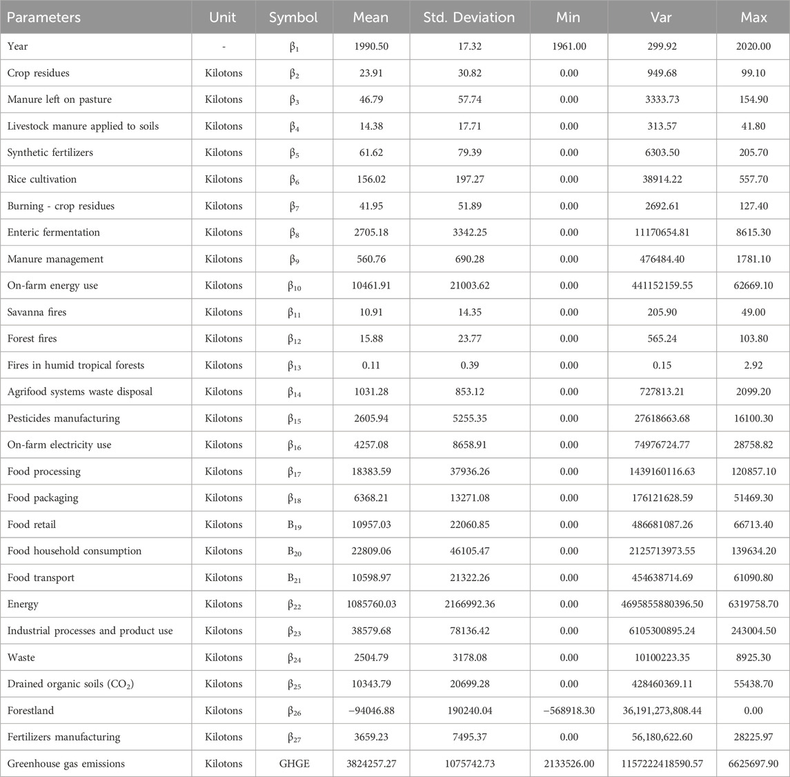
Table 1. Statistical analysis of a dataset comprising 8,100 data points obtained from the FAOSTAT for prediction of GHGE.

Figure 1

Figure 1. Schematic representation of key stakeholder involvement in the evolution of greenhouse gas emissions in the expansive agrifood system.

Addressing limitations in input data is crucial for reliable model performance in the preprocessing stage of data-based models and machine learning algorithms. Missing data, for instance, is often managed through imputation techniques (mean, median) or, when minimal, by data removal. Outliers, which can distort model understanding, are typically identified using statistical measures or visualizations and either removed or capped.

Feature scaling (normalization) is essential for models sensitive to feature magnitudes, ensuring consistent data contributions.

Feature engineering can also play a vital role by transforming data to capture relationships better, enhancing the model’s input data quality. These preprocessing steps enhance data quality and structure, providing a solid foundation for practical model training and deployment.

3.2 Machine learning models

Machine learning algorithms represent computational models specifically formulated for the iterative extraction of patterns and relationships from data, facilitating predictive or decision-making capabilities without explicit programming. These algorithms harness statistical methodologies to enhance a pre-established objective function by iteratively adjusting internal parameters in response to training examples. Supervised learning algorithms, exemplified by support vector machines or neural networks, acquire mappings from input data to desired outputs. Conversely, unsupervised learning algorithms, such as clustering or dimensionality reduction methods, elucidate intrinsic structures and patterns within data by exploring inherent relationships.

3.2.1 Random forest (RF)

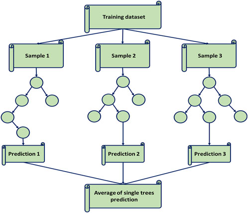
The Random Forest (RF) algorithm is a committee-based decision-making approach where each decision-maker is represented as a tree (Hajipour et al., 2020). Unlike single-unit reliance, RF utilizes a group, or “forest,” of decision trees for prediction (Huynh-Cam et al., 2021). Each tree is trained on a random subset of the data and may consider only a random subset of features during decision-making (Shaikhina et al., 2019). This randomness prevents overfitting, ensuring the model generalizes well to new and unseen data. Various sources have extensively described the mathematical model and structure of the RF machine-learning algorithm (Su et al., 2021). Figure 2 shows the illustration of the RF.

Figure 2

Figure 2. Diagram illustrating the procedural flow of the RF algorithm.

3.2.2 Long-short term memory (LSTM)

In machine learning algorithms, a notable performer in time series data analysis is the Recurrent Neural Network (RNN) architecture (Essien and Giannetti, 2020). Distinguished by its ability to incorporate historical information and discern patterns for predictive modeling, the RNN, nonetheless, grapples with the challenge of managing an extensive repository of historical data, potentially resulting in information saturation and gradual deterioration. To address this concern, a specialized variant of the RNN architecture, known as Long Short-Term Memory (LSTM), has been carefully devised (Fu, 2020). The LSTM architecture strategically preserves pertinent information while efficiently discarding irrelevant data, enhancing information processing and modeling precision within the temporal context (Kumar et al., 2023).

Given the nature of the research on predicting future climate scenarios in agrifood systems using machine learning, a combination of time series forecasting models and regression models is recommended. Specifically, this research considers models like LSTM networks, which are well-suited for handling sequential data over time, and RF, which can capture complex relationships within the dataset (Sahoo et al., 2019). The choice of LSTM is logical due to the temporal aspect of the dataset spanning from 1961 to 2020. LSTMs are adept at capturing temporal dependencies and can effectively model the time series nature of GHGE (Hamdan et al., 2023). This is important for understanding trends and predicting in a dynamic system like agrifood. Additionally, RF can complement the LSTM model by capturing non-linear relationships and interactions among factors influencing emissions. Given the multidimensional nature of agrifood systems, RFs can handle the complexity arising from diverse variables such as regional variations, socioeconomic factors, and technological advancements.

The LSTM model is a well-known architecture with remarkable performance in handling complex sequential computations (Figure 3) (Mohan and Gaitonde, 2018). This algorithm’s foundational structure, detection mechanisms, and the mathematical and logical relationships governing its functionality have been extensively documented in reputable sources like Xue et al. (2018) (Xue et al., 2018).

Figure 3

Figure 3. Diagram illustration of the procedural flow of the LSTM algorithm.

3.2.3 Hybrid machine learning algorithm architecture

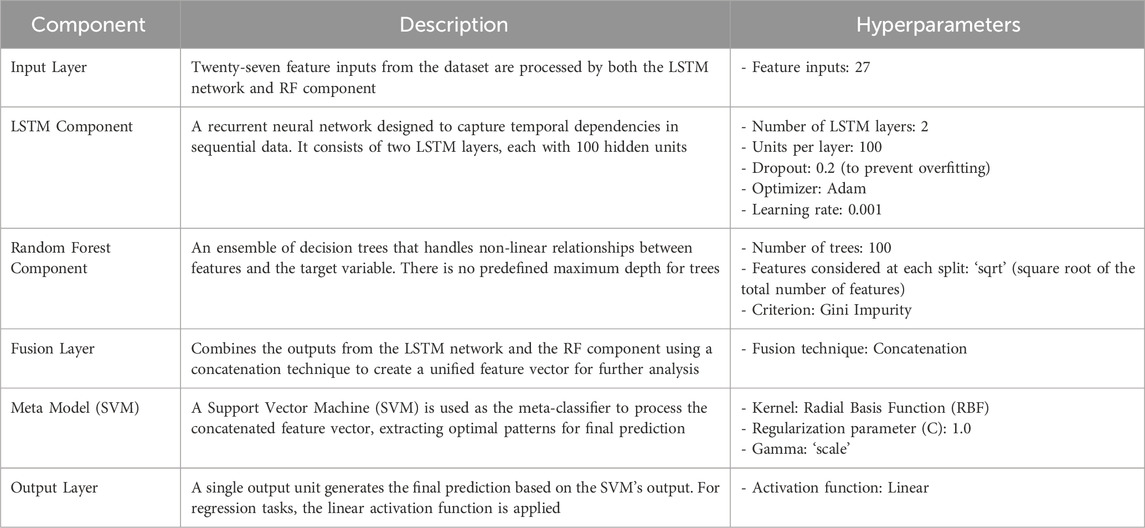
We would use a stacked ensemble approach to construct an architecture that integrates LSTM networks and RF models (Hu and Shi, 2020). This technique entails layering models so that the predictions from the LSTM and RF models are used as inputs into a subsequent subsidiary model (Shen et al., 2022). This overall structure concurrently combines predictions from the LSTM and RF models, and a meta-model is used to synthesize these predictions and make the final decision (Cao et al., 2023). Hyperparameters are systematically optimized using cross-validation techniques to find the optimal configuration for this specific dataset (Cao et al., 2023). Careful application of validation and regularization mechanisms during LSTM training mitigates the risk of overfitting and enhances computational efficiency in this complex ensemble model’s training and inference stages.

The LSTM-RF hybrid model architecture consists of two LSTM layers, each with 100 hidden units, designed to capture sequential patterns in the data, with a dropout rate of 0.2 applied between layers to prevent overfitting. The model uses the Adam optimizer for fast convergence, with a learning rate 0.001. The Random Forest (RF) component comprises 100 trees, and the maximum tree depth is unrestricted to capture complex interactions, using the “sqrt” option to determine the number of features at each split. The outputs of both the LSTM and RF models are combined via concatenation in the fusion layer, creating a comprehensive feature vector that integrates both sequential and non-sequential patterns. This combined vector is processed by a Support Vector Machine (SVM) meta-classifier with an RBF kernel, where the regularization parameter (C) is set to 1.0 to control overfitting, and the gamma parameter is set to “scale” to adjust to the data. Finally, the output layer generates the model’s prediction using a linear activation function, which can be applied to either regression tasks or classification, depending on the problem. Table 2 presents the model structure architecture and hyperparameters applied in the hybrid model structure.

Table 2

Table 2. Hybrid model LSTM-RF architecture and hyperparameters.

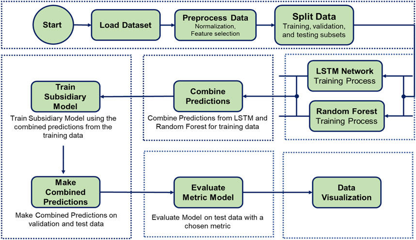
Figure 4 shows the architecture of the hybrid model and the step-by-step flowchart of the proposed machine-learning model. As this is a complex ensemble model, careful attention should be given to the risk of overfitting and computational efficiency during the training and inference stages. To further prevent overfitting, it may also be helpful to use a validation and early stopping mechanism during the training of the LSTM.

Figure 4

Figure 4. Diagram illustration of the flow diagram for the LSTM-RF HML algorithm.

The implemented hybrid neural network architecture integrates LSTM and RF models through ensemble stacking, enhancing prediction accuracy by combining temporal and non-temporal feature extraction. The process begins with extensive data preprocessing, including normalization and reshaping for time-series data. In the LSTM pathway, a stacked LSTM network captures sequential dependencies, producing an output vector that encodes temporal features. At the same time, the RF model processes non-temporal data, generating predictions through an ensemble of decision trees. These outputs are fused in a dedicated layer through a simple concatenation mechanism, creating a rich, integrated feature set. This combined input is fed into the meta-model, a traditional support vector machine (SVM), to generate the final prediction for regression tasks. The data is split into training, validation, and test sets, with the LSTM capturing temporal dependencies using multiple LSTM cells and the RF identifying non-linear relationships between features and the target variable. The concatenated outputs from both models form a more extended feature vector, which the SVM meta-model processes to extract optimal patterns for the final prediction, made through a linear activation function. When a new sample is introduced, the LSTM and RF models process it, their output vectors are combined, and the SVM meta model makes the final prediction. Figure 5 illustrates the flow diagram for the LSTM-RF hybrid machine learning (HML) algorithm.

Figure 5

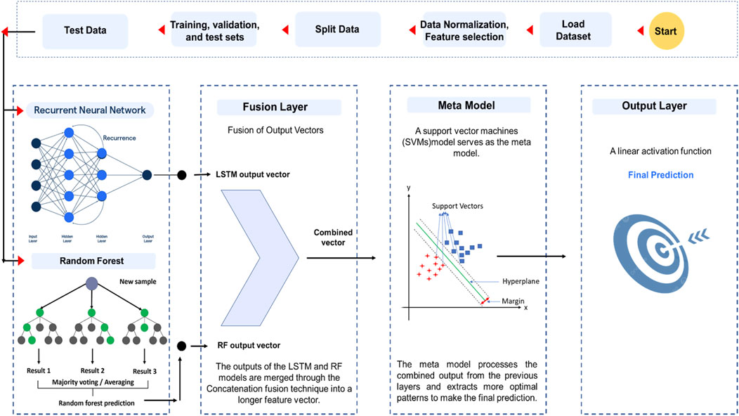
Figure 5. Illustration of the structure of preprocessing and the flow diagram for the LSTM-RF HML algorithm.

3.3 Evaluation metrics

To evaluate the results of artificial intelligence in predicting GHGE and establish a suitable measure for comparison, one can refer to a set of standard statistical measures presented in Formulas 1–5. The relevant information linked to these formulas includes Mean Average Deviation (MAD), Root Mean Square Error (RMSE), Standard Deviation (SD), Correlation Coefficient (R²), and Absolute Mean Average Deviation (AMAD). These measures play an essential role in assessing the effectiveness and accuracy of AI models in GHGE prediction. By using MAD, RMSE, SD, R², and AMAD, valuable insights into the model’s predictive abilities and performance against benchmarks can be obtained. These measures collectively contribute to a thorough evaluation, providing a nuanced understanding of the AI model’s reliability in predicting GHGE.

$RMSE=\sqrt{\frac{1}{n}{\displaystyle \sum _{i=1}^n}{\left({{GHGE}_{meas.}}_i-{{GHGE}_{pred.}}_i\right)}^2}(1)$

$MAD=\frac{{\displaystyle \sum _{i=1}^n}{\frac{{GHGE}_{meas.}-{GHGE}_{pred.}}{{GHGE}_{meas.}}}_i}{n}\times 100(2)$

$SD=\sqrt{\frac{{\displaystyle \sum _{i=1}^n}{\left({\left(\frac{{GHGE}_{meas.}-{GHGE}_{pred.}}{{GHGE}_{meas.}}\right)}_i-{\left(\frac{{GHGE}_{meas.}-{GHGE}_{pred.}}{{GHGE}_{meas.}}\right)}_{mean}\right)}^2}{n-1}}(3)$

$R^2=1-\frac{{\displaystyle \sum _{i=1}^n}{\left({{GHGE}_{meas.}}_i-{{GHGE}_{pred.}}_i\right)}^2}{{\displaystyle \sum _{i=1}^n}{\left({{GHGE}_{pred.}}_i-\frac{{\displaystyle \sum _{i=1}^n}{GHGE}_{meas.}}{n}\right)}^2}(4)$

$AMAD=\frac{{\displaystyle \sum _{i=1}^n}\left|{\frac{{GHGE}_{meas.}-{GHGE}_{pred.}}{{GHGE}_{meas.}}\times 100}_i\right|}{n}(5)$

3.4 Cross validation

The k-fold cross-validation method can be applied to validate and fine-tune the outcomes of ML and DL algorithms. This method utilizes the 2^S rule, where “S” is the number of variables, to ensure robust test data validation. The ML and HML models were used in this process. The k-fold method was used, with “k” set to 6 for this dataset. Specifically, one set out of 8 was designated for testing, while the other seven were used for training. The ML and HML algorithms underwent ten evaluations to choose each subset, resulting in 60 evaluations. Ultimately, the model with the lowest RMSE value was selected to predict GHGE. The validation sequence for this paper is illustrated in Figure 6.

Figure 6

Figure 6. Schematic illustration of the flow diagram for k-fold cross-validation.

4 Result and discussion

4.1 Evaluation errors and their impact

Researchers from various fields have shown a strong interest in Hybrid Machine Learning (HML) models due to their impressive ability to address regression problems. This article used 2 ML algorithms (LSTM and RF) and one HML algorithm (LSTM-RF) to predict GHGE. The GHGE prediction results for these algorithms are thoroughly presented in Table 3. The information contained in these tables provides a comprehensive overview of GHGE predictions using HML compared to traditional ML algorithms across test, training, and validation datasets. The findings detailed in Table 3 offer an in-depth analysis of the predictive performance of HML and simple ML algorithms, demonstrating their effectiveness in handling GHGE prediction tasks across various datasets.

Table 3

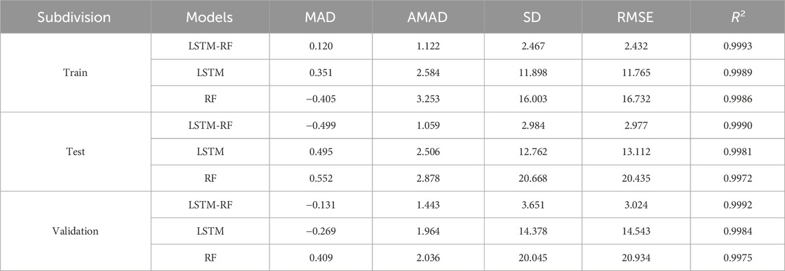
Table 3. Performance metrics of ML and HML models in prediction of GHGE accuracy on the testing, training, and validation subdivision.

A careful look at Table 3 shows that the performance accuracy of the LSTM-RF HML algorithm, a hybrid algorithm, exceeds that of conventional LSTM and RF algorithms. Specifically, the LSTM-RF HML algorithm demonstrates the following results for train data: MAD = 0.120%, AMAD = 1.122%, SD = 2.467, RMSE = 2.432, and R² = 0.9993. Similarly, for test data, the algorithm produces MAD = −0.499%, AMAD = 1.059%, SD = 2.984, RMSE = 2.977, and R² = 0.9990. In the validation data, the recorded values are MAD = −0.131%, AMAD = 1.443%, SD = 3.651, RMSE = 3.024, and R² = 0.9992. These findings support the conclusion that the performance accuracy of the LSTM-RF HML algorithm surpasses both LSTM and RF algorithms. The simplicity of the presented results reinforces the comparison.

4.2 Evaluation graphical results for prediction of GHGE

Figure 7 presents a chart comparing each data record’s measured and predicted GHGE. It provides information on most of the data, including both test and validation sets. The visual analysis of Figure 7 demonstrates that the HML LSTM-RF algorithm exhibits superior performance accuracy compared to the traditional RF and LSTM algorithms. This representation aids in assessing the correlation coefficient. Examining the outcomes presented in Table 3 and Figure 7, it becomes evident that the hierarchy of algorithm performance for GHGE prediction is LSTM-RF > LSTM > RF, based on their respective performance accuracies.

Figure 7

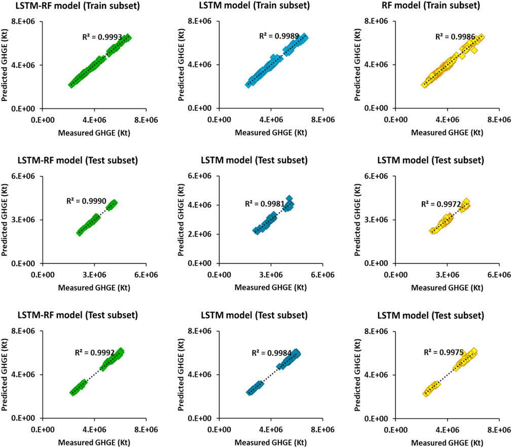
Figure 7. A comparison between measured and predicted GHGE values for the training, testing, and validation subset by the three evaluated ML and HML models.

Figure 8 displays a histogram of errors when predicting GHGE values using 3 ML and HML models. The figure shows that the performance accuracy of the LSTM-RF algorithm surpasses that of other algorithms. The error distribution in the figure is symmetrical around the zero point, indicating a normal error distribution without positive or negative biases. Additionally, it is noticeable in the figure that RF and LSTM algorithms lack symmetry and exhibit lower performance compared to the LSTM-RF HML algorithm.

Figure 8

Figure 8. Displaying histograms of prediction errors in GHGE and theoretical normal distributions represented by red lines.

Figure 9 displays two important statistical parameters and metrics for evaluating ML algorithms through reviews and quantitative comparisons. The figure presents RMSE and R2 values for predicting GHGE in the test subset. Analyzing these figures allows us to understand how the RMSE and R² values change about each other, providing insight into this critical parameter. After investigating these two aspects, it becomes evident that the performance accuracy of the algorithms discussed in this article follows this order: LSTM-RF > LSTM > RF. These results highlight that the accuracy of the HML algorithm surpasses that of traditional ML algorithms. Properly utilizing these HML algorithms can offer insights into significant changes and consequences affecting food systems and the interconnected network of agriculture, food production, and supply. This can help prevent many problems through effective management of food resource reduction.

Figure 9

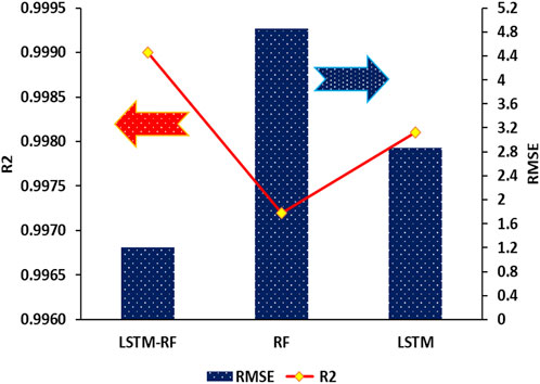
Figure 9. Evaluating the prediction efficacy of ML models (LSTM and RF) and HML models (LSTM- RF) on the testing subset by comparing RMSE and R² values in the GHGE prediction.

One effective method to assess and compare algorithm performance is Score Analysis (SA). This approach assigns a numerical score to each statistical calculation value for every computational and statistical method used in the algorithms. A higher score indicates greater performance accuracy, while a lower score signifies reduced accuracy. Subsequently, these values are aggregated for the training, test, and validation subsets. The algorithm with the highest total score demonstrates superior performance accuracy compared to the others. In this investigation, the maximum score is 9, and the minimum is 1 (Table 4). After calculating this score, it is determined that the total scores for LSTM-RF, LSTM, and RF algorithms are 116, 69, and 40, respectively. Upon analyzing these scores, it is clear that the LSTM-RF algorithm exhibits higher accuracy than the other two, while the RF algorithm shows the lowest accuracy (Figure 10).

Table 4

Table 4. Performance score analysis of ML and HML models in prediction of GHGE accuracy on the testing, training, and validation subdivision.

Figure 10

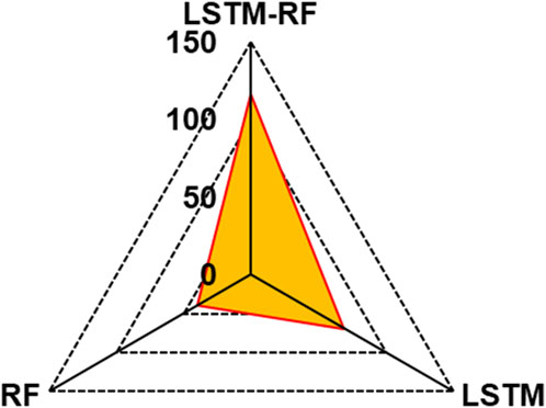
Figure 10. Comparative spider diagram showcasing the prediction performance of ML (LSTM and RF) and HML (LSTM-RF) models for GHGE prediction based on score analysis. Scores are delineated for the summation of the training, testing, and validation subsets, as well as the cumulative total score.

One factor used to understand the importance of input variables about the output variables is Pearson’s coefficient (R). This coefficient, ranging from −1 to +1, reveals the strength and direction of correlations. A +1 value indicates a direct solid correlation, while −1 signifies a robust inverse correlation. A value close to 0 suggests no correlation for GHGE output. Equation 6 illustrates the Pearson coefficient.

$R=\frac{{\displaystyle \sum _{i=1}^n}\left({\theta }_i-\overline{\theta }\right)\left({ϵ}_i-\overline{ϵ}\right)}{\sqrt{{\displaystyle \sum _{i=1}^n}{\left({\theta }_i-\overline{\theta }\right)}^2}\sqrt{{\displaystyle \sum _{i=1}^n}{\left({ϵ}_i-\overline{ϵ}\right)}^2}}(6)$

R is the Pearson correlation, and θ and ϵ are the rank of each variable dataset. A heat map is a visual representation that helps assess these important input variable parameters. To simplify the heat map’s design, we have used symbolic names (β₁- β₂₇ and GHGE) shown in Table 1 for the input variables due to the length of their names. This approach enables a more straightforward presentation of the heat map’s new configuration. After analyzing the heat map, it is evident that some input variables have a direct relationship, while others have an inverse relationship with the GHGE output. Input variables (β₂-β₉, β₁₁-β₁₃, β₂₄, and β₂₆) can be associated with negative correlations, while input variables (β₁, β₁₀, β₁₄-β₂₃, β₂₅, and β₂₇) are linked with positive correlations (Figure 11). These relationships can be expressed using Equations 7, 8:

$\text{GHGE}\propto {{\mathrm{\beta }}_1,\mathrm{\beta }}_{10},{\mathrm{\beta }}_{14}-{\mathrm{\beta }}_{23},{\mathrm{\beta }}_{25},{\mathrm{\beta }}_{27}(7)$

$\text{GHGE}\propto \frac{1}{{\mathrm{\beta }}_2-{\mathrm{\beta }}_9,{\mathrm{\beta }}_{11}-{\mathrm{\beta }}_{13},{\mathrm{\beta }}_{24},{\mathrm{\beta }}_{26}}(8)$

Figure 11

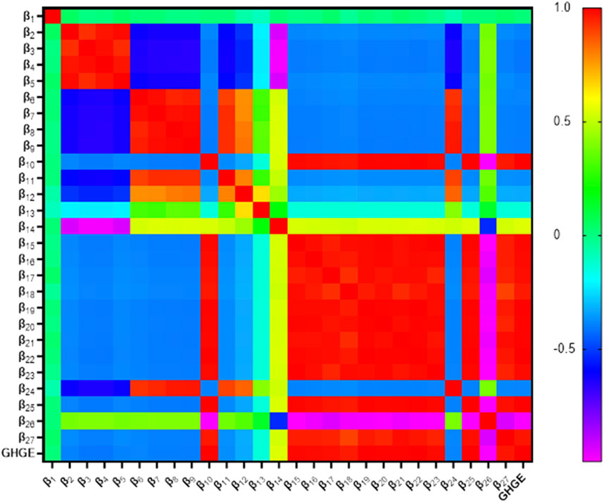
Figure 11. A visual heat map plot illustrating the determination of the 27 input variables and GHGE.

Notably, values of β₉ (on-farm energy use), β₁₄-β₂₂ (pesticides manufacturing, on-farm electricity use, food processing, food packaging, food retail, food household consumption, food transport, energy, and industrial processes and product use), and β₂₄-β₂₆ (drained organic soils (Co₂), forestland and fertilizers manufacturing) have a highly significant impact on the GHGE output. Comparing Pearson’s coefficient with the heat map provides valuable insights into how the data is related and their influence on the GHGE output.

5 Limitation

A significant limitation of the input data stems from its dependence on aggregated national estimates, which can obscure regional differences within countries and result in less accurate local insights. This broad aggregation can hide crucial emission profile variations influenced by differing agricultural practices, land use patterns, and climatic conditions across various regions. For example, emissions from livestock can significantly vary between arid and temperate climates, yet national averages may need to capture these differences, leading to potentially misguided policy responses. Furthermore, the dataset employs a Tier 1 methodology for emissions estimation, relying on default emission factors that do not account for specific agricultural practices, local environmental contexts, or recent technological advancements. Consequently, this approach may need to include vital details regarding resource efficiency and the effects of innovative farming methods that could substantially influence emissions levels. These crucial developments need to be adequately represented in older datasets. Furthermore, there is the risk of reporting inconsistencies and methodological variations among countries, leading to emissions quantification and reporting discrepancies. This lack of standardization introduces uncertainties, particularly when comparing emissions data across different countries or regions.

6 Conclusion

In conclusion, comprehending the complex relationship between climate change and agrifood systems is essential for assessing the long-term implications on food production and sustainability. This study underscores the necessity of accurately forecasting greenhouse gas emissions (GHGE) from agricultural practices to devise strategies that simultaneously address food security and environmental concerns. By utilizing advanced machine learning techniques—specifically, long-term term Memory (LSTM), Random Forest (RF), and a hybrid LSTM-RF model—, we have significantly improved our predictive abilities concerning future climate scenarios linked to GHGE within the agricultural sector. The analysis utilized a comprehensive dataset comprising 8,100 data points across 27 input features, which capture various elements of the agrifood system’s contribution to greenhouse emissions, covering the years 1961–2020. Remarkably, the LSTM-RF hybrid model surpassed the individual models’ predictive accuracy, achieving a Root Mean Square Error (RMSE) of 2.977 and an R² value of 0.9990. This performance demonstrates its proficiency in capturing intricate temporal dependencies and interactions in the data. As revealed by Pearson correlation analysis, key determinants influencing GHGE include on-farm energy consumption, pesticide manufacturing activities, electricity usage, and land use, such as drained organic soils and forestland. Despite these encouraging findings, the study acknowledges several limitations. The dataset is confined to historical data from 1961 to 2020, suggesting that updating it with more recent information could enhance predictive accuracy regarding evolving agrifood systems.

Furthermore, the model’s effectiveness hinges on the quality of input data, which may need to be corrected or corrected in historical emissions records. The dependence on past data also restricts the model’s capacity to anticipate unexpected occurrences, such as advancements in agricultural technology or sudden climate changes. Although the hybrid LSTM-RF algorithm demonstrates substantial efficacy, there is room for further refinement to enhance its generalizability across diverse agricultural systems and climatic regions. This indicates promising avenues for future research, including integrating real-time data, enhancing the algorithm’s flexibility for various agrifood systems, and broadening the scope of the study to incorporate additional environmental factors influencing GHGE beyond those currently considered.

Data availability statement

The data analyzed in this study is subject to the following licenses/restrictions: The corresponding authors are open to granting access to the data upon reasonable requests made for academic purposes. Requests to access these datasets should be directed to Hamzeh Ghorbani; aGFtemVoZ2hvcmJhbmk2OEB5YWhvby5jb20=.

Author contributions

OB: Conceptualization, Data curation, Formal Analysis, Funding acquisition, Investigation, Methodology, Project administration, Resources, Software, Validation, Visualization, Writing–original draft, Writing–review and editing. HGH: Conceptualization, Data curation, Formal Analysis, Funding acquisition, Investigation, Methodology, Project administration, Resources, Software, Supervision, Validation, Visualization, Writing–original draft, Writing–review and editing.

Funding

The author(s) declare that no financial support was received for the research, authorship, and/or publication of this article.

Conflict of interest

The authors confirm that no financial conflicts of interest or personal relationships might have affected the outcomes reported in this paper.

Publisher’s note

All claims expressed in this article are solely those of the authors and do not necessarily represent those of their affiliated organizations, or those of the publisher, the editors and the reviewers. Any product that may be evaluated in this article, or claim that may be made by its manufacturer, is not guaranteed or endorsed by the publisher.

References

Aguilera, E., Reyes-Palomo, C., Díaz-Gaona, C., Sanz-Cobena, A., Smith, P., García-Laureano, R., et al. (2021). Greenhouse gas emissions from Mediterranean agriculture: evidence of unbalanced research efforts and knowledge gaps. Glob. Environ. Change 69, 102319. doi:10.1016/j.gloenvcha.2021.102319

CrossRef Full Text | Google Scholar

Ahmed, M., Asif, M., Sajad, M., Khattak, J. Z. K., Ijaz, W., Wasaya, A., et al. (2013). Could agricultural system be adapted to climate change? a review. Aust. J. Crop Sci. 7 (11), 1642–1653.

Google Scholar

Cammarata, M., Timpanaro, G., Incardona, S., La Via, G., and Scuderi, A. (2023). The quantification of carbon footprints in the agri-food sector and future trends for carbon sequestration: a systematic literature review. Sustainability 15 (21), 15611. doi:10.3390/su152115611

CrossRef Full Text | Google Scholar

Cao, M., Mao, K., Bateni, S. M., Jun, C., Shi, J., Du, Y., et al. (2023). Granulation-based LSTM-RF combination model for hourly sea surface temperature prediction. Int. J. Digital Earth 16 (1), 3838–3859. doi:10.1080/17538947.2023.2260779

CrossRef Full Text | Google Scholar

Chen, M., Qian, Z., Boers, N., Jakeman, A. J., Kettner, A. J., Brandt, M., et al. (2023). Iterative integration of deep learning in hybrid Earth surface system modelling. Nat. Rev. Earth and Environ. 4 (8), 568–581. doi:10.1038/s43017-023-00452-7

CrossRef Full Text | Google Scholar

Costa, C., Wollenberg, E., Benitez, M., Newman, R., Gardner, N., and Bellone, F. (2022). Roadmap for achieving net-zero emissions in global food systems by 2050. Sci. Rep. 12 (1), 15064. doi:10.1038/s41598-022-18601-1

PubMed Abstract | CrossRef Full Text | Google Scholar

Crane-Droesch, A. (2018). Machine learning methods for crop yield prediction and climate change impact assessment in agriculture. Environ. Res. Lett. 13 (11), 114003. doi:10.1088/1748-9326/aae159

CrossRef Full Text | Google Scholar

Devendra, C. (2012). Climate change threats and effects: challenges for agriculture and food security. Malaysia: Academy of Sciences Malaysia.

Google Scholar

Dhanya, P., Ramachandran, A., and Palanivelu, K. (2022). Understanding the local perception, adaptation to climate change and resilience planning among the farmers of semi-arid tracks of South India. Agric. Res. 11, 291–308. doi:10.1007/s40003-021-00560-0

CrossRef Full Text | Google Scholar

Durán-Sandoval, D., Uleri, F., Durán-Romero, G., and López, A. M. (2023). Food, climate change, and the challenge of innovation. Encyclopedia 3 (3), 839–852. doi:10.3390/encyclopedia3030060

CrossRef Full Text | Google Scholar

Essien, A., and Giannetti, C. (2020). A deep learning model for smart manufacturing using convolutional LSTM neural network autoencoders. IEEE Trans. Industrial Inf. 16 (9), 6069–6078. doi:10.1109/tii.2020.2967556

CrossRef Full Text | Google Scholar

Fan, C., Nie, S., Li, H., Pan, Q., Shi, X., Qin, S., et al. (2024). Geological characteristics and major factors controlling the high yield of tight oil in the Da’anzhai member of the western Gongshanmiao in the central Sichuan basin, China. Geomechanics Geophys. Geo-Energy Geo-Resources 10 (1), 67. doi:10.1007/s40948-024-00783-9

CrossRef Full Text | Google Scholar

Frame, D. J., Rosier, S. M., Noy, I., Harrington, L. J., Carey-Smith, T., Sparrow, S. N., et al. (2020). Climate change attribution and the economic costs of extreme weather events: a study on damages from extreme rainfall and drought. Clim. Change 162, 781–797. doi:10.1007/s10584-020-02729-y

CrossRef Full Text | Google Scholar

Fu, Y. (2020). Modeling, prediction and control of engineering systems with long short-term memory.

Google Scholar

Gaitán, C. F. (2020). “Machine learning applications for agricultural impacts under extreme events,” in Climate extremes and their implications for impact and risk assessment (Elsevier), 119–138.

Google Scholar

Ghil, M., and Lucarini, V. (2020). The physics of climate variability and climate change. Rev. Mod. Phys. 92 (3), 035002. doi:10.1103/revmodphys.92.035002

CrossRef Full Text | Google Scholar

Giamouri, E., Zisis, F., Mitsiopoulou, C., Christodoulou, C., Pappas, A. C., Simitzis, P. E., et al. (2023). Sustainable strategies for greenhouse gas emission reduction in small ruminants farming. Sustainability 15 (5), 4118. doi:10.3390/su15054118

CrossRef Full Text | Google Scholar

Hajipour, F., Jozani, M. J., and Moussavi, Z. (2020). A comparison of regularized logistic regression and random forest machine learning models for daytime diagnosis of obstructive sleep apnea. Med. and Biol. Eng. and Comput. 58, 2517–2529. doi:10.1007/s11517-020-02206-9

PubMed Abstract | CrossRef Full Text | Google Scholar

Hamdan, A., Al-Salaymeh, A., AlHamad, I. M., Ikemba, S., and Ewim, D. R. E. (2023). Predicting future global temperature and greenhouse gas emissions via LSTM model. Sustain. Energy Res. 10 (1), 21. doi:10.1186/s40807-023-00092-x

CrossRef Full Text | Google Scholar

Hamrani, A., Akbarzadeh, A., and Madramootoo, C. A. (2020). Machine learning for predicting greenhouse gas emissions from agricultural soils. Sci. Total Environ. 741, 140338. doi:10.1016/j.scitotenv.2020.140338

PubMed Abstract | CrossRef Full Text | Google Scholar

Hu, W., and Shi, Y. (2020). Prediction of online consumers’ buying behavior based on LSTM-RF model, 224, 228. doi:10.1109/ccisp51026.2020.9273501

CrossRef Full Text | Google Scholar

Huynh-Cam, T.-T., Chen, L.-S., and Le, H. (2021). Using decision trees and random forest algorithms to predict and determine factors contributing to first-year university students’ learning performance. Algorithms 14 (11), 318. doi:10.3390/a14110318

CrossRef Full Text | Google Scholar

Kalt, G., Mayer, A., Haberl, H., Kaufmann, L., Lauk, C., Matej, S., et al. (2021). Exploring the option space for land system futures at regional to global scales: the diagnostic agro-food, land use and greenhouse gas emission model BioBaM-GHG 2.0. Ecol. Model. 459, 109729. doi:10.1016/j.ecolmodel.2021.109729

CrossRef Full Text | Google Scholar

Koul, B., Yakoob, M., and Shah, M. P. (2022). Agricultural waste management strategies for environmental sustainability. Environ. Res. 206, 112285. doi:10.1016/j.envres.2021.112285

PubMed Abstract | CrossRef Full Text | Google Scholar

Kumar, I., Tripathi, B. K., and Singh, A. (2023). Attention-based LSTM network-assisted time series forecasting models for petroleum production. Eng. Appl. Artif. Intell. 123, 106440. doi:10.1016/j.engappai.2023.106440

CrossRef Full Text | Google Scholar

Kumari, S., Fagodiya, R. K., Hiloidhari, M., Dahiya, R. P., and Kumar, A. (2020). Methane production and estimation from livestock husbandry: a mechanistic understanding and emerging mitigation options. Sci. Total Environ. 709, 136135. doi:10.1016/j.scitotenv.2019.136135

PubMed Abstract | CrossRef Full Text | Google Scholar

Lamine, C. (2015). Sustainability and resilience in agrifood systems: reconnecting agriculture, food and the environment. Sociol. Rural. 55 (1), 41–61. doi:10.1111/soru.12061

CrossRef Full Text | Google Scholar

Lobell, D. B., and Gourdji, S. M. (2012). The influence of climate change on global crop productivity. Plant physiol. 160 (4), 1686–1697. doi:10.1104/pp.112.208298

PubMed Abstract | CrossRef Full Text | Google Scholar

Meena, R. S., Kumar, S., and Yadav, G. S. (2020) “Soil carbon sequestration in crop production,” in Nutrient dynamics for sustainable crop production, 1–39.

CrossRef Full Text | Google Scholar

Minoofar, A., Gholami, A., Eslami, S., Hajizadeh, A., Gholami, A., Zandi, M., et al. (2023). Renewable energy system opportunities: a sustainable solution toward cleaner production and reducing carbon footprint of large-scale dairy farms. Energy Convers. Manag. 293, 117554. doi:10.1016/j.enconman.2023.117554

CrossRef Full Text | Google Scholar

Mohan, A. T., and Gaitonde, D. V. (2018). A deep learning based approach to reduced order modeling for turbulent flow control using LSTM neural networks. arXiv Prepr. arXiv:1804.09269. doi:10.48550/arXiv.1804.09269

CrossRef Full Text | Google Scholar

Nath, P. C., Mishra, A. K., Sharma, R., Bhunia, B., Mishra, B., Tiwari, A., et al. (2024). Recent advances in artificial intelligence towards the sustainable future of agri-food industry. Food Chem. 447, 138945. doi:10.1016/j.foodchem.2024.138945

PubMed Abstract | CrossRef Full Text | Google Scholar

Notarnicola, B., Sala, S., Anton, A., McLaren, S. J., Saouter, E., and Sonesson, U. (2017). The role of life cycle assessment in supporting sustainable agri-food systems: a review of the challenges. J. Clean. Prod. 140, 399–409. doi:10.1016/j.jclepro.2016.06.071

CrossRef Full Text | Google Scholar

Olivier, J. G. J., and Peters, J. A. H. W. (2005). CO2 from non-energy use of fuels: a global, regional and national perspective based on the IPCC Tier 1 approach. Resour. Conservation Recycl. 45 (3), 210–225. doi:10.1016/j.resconrec.2005.05.008

CrossRef Full Text | Google Scholar

Pasrija, P., Jha, P., Upadhyaya, P., Khan, M., and Chopra, M. (2022). Machine learning and artificial intelligence: a paradigm shift in big data-driven drug design and discovery. Curr. Top. Med. Chem. 22 (20), 1692–1727. doi:10.2174/1568026622666220701091339

PubMed Abstract | CrossRef Full Text | Google Scholar

Raimi, M. O., Vivien, O. T., and Oluwatoyin, O. A. (2021) “Creating the healthiest nation: climate change and environmental health impacts in Nigeria: a narrative review,” in Morufu olalekan raimi, tonye vivien odubo and adedoyin oluwatoyin omidiji (2021) creating the healthiest nation: climate change and environmental health impacts in Nigeria: a narrative review. Scholink sustainability in environment. Valencia, Spain: ISSN.

CrossRef Full Text | Google Scholar

Ramankutty, N., Mehrabi, Z., Waha, K., Jarvis, L., Kremen, C., Herrero, M., et al. (2018). Trends in global agricultural land use: implications for environmental health and food security. Annu. Rev. plant Biol. 69, 789–815. doi:10.1146/annurev-arplant-042817-040256

PubMed Abstract | CrossRef Full Text | Google Scholar

Raza, A., Razzaq, A., Mehmood, S. S., Zou, X., Zhang, X., Lv, Y., et al. (2019). Impact of climate change on crops adaptation and strategies to tackle its outcome: a review. Plants 8 (2), 34. doi:10.3390/plants8020034

PubMed Abstract | CrossRef Full Text | Google Scholar

Rubanga, D. P., Hatanaka, K., and Shimada, S. (2019). Development of a simplified smart agriculture system for small-scale greenhouse farming. Sensors and Mater. 31, 831. doi:10.18494/sam.2019.2154

CrossRef Full Text | Google Scholar

Saha, N. D., Chakrabarti, B., Bhatia, A., Jain, N., Sharma, A., and Gurjar, D. S. (2022). “Greenhouse gas (GHG) emission mitigation options: an approach towards climate smart agriculture,” in Innovative approaches for sustainable development: theories and practices in agriculture (Springer), 43–63.

CrossRef Full Text | Google Scholar

Sahoo, B. B., Jha, R., Singh, A., and Kumar, D. (2019). Long short-term memory (LSTM) recurrent neural network for low-flow hydrological time series forecasting. Acta Geophys. 67 (5), 1471–1481. doi:10.1007/s11600-019-00330-1

CrossRef Full Text | Google Scholar

Santoso, I., Purnomo, M., Sulianto, A. A., and Choirun, A. (2021). Machine learning application for sustainable agri-food supply chain performance: a review. IOP Conf. Ser. Earth Environ. Sci. 924, 012059. doi:10.1088/1755-1315/924/1/012059

CrossRef Full Text | Google Scholar

Sarfraz, M., Iqbal, K., Wang, Y., Bhutta, M. S., and Jaffri, Z. u. A. (2023). Role of agricultural resource sector in environmental emissions and its explicit relationship with sustainable development: evidence from agri-food system in China. Resour. Policy 80, 103191. doi:10.1016/j.resourpol.2022.103191

CrossRef Full Text | Google Scholar

Sarma, H. H., Borah, S. K., Dutta, N., Sultana, N., Nath, H., and Das, B. C. (2024). Innovative approaches for climate-resilient farming: strategies against environmental shifts and climate change. Int. J. Environ. Clim. Change 14 (9), 217–241. doi:10.9734/ijecc/2024/v14i94407

CrossRef Full Text | Google Scholar

Schewe, J., Gosling, S. N., Reyer, C., Zhao, F., Ciais, P., Elliott, J., et al. (2019). State-of-the-art global models underestimate impacts from climate extremes. Nat. Commun. 10 (1), 1005. doi:10.1038/s41467-019-08745-6

PubMed Abstract | CrossRef Full Text | Google Scholar

Shafi, U., Mumtaz, R., García-Nieto, J., Hassan, S. A., Zaidi, S. A. R., and Iqbal, N. (2019). Precision agriculture techniques and practices: from considerations to applications. Sensors 19 (17), 3796. doi:10.3390/s19173796

PubMed Abstract | CrossRef Full Text | Google Scholar

Shaikhina, T., Lowe, D., Daga, S., Briggs, D., Higgins, R., and Khovanova, N. (2019). Decision tree and random forest models for outcome prediction in antibody incompatible kidney transplantation. Biomed. Signal Process. Control 52, 456–462. doi:10.1016/j.bspc.2017.01.012

CrossRef Full Text | Google Scholar

Shen, Y., Mercatoris, B., Cao, Z., Kwan, P., Guo, L., Yao, H., et al. (2022). Improving wheat yield prediction accuracy using LSTM-RF framework based on UAV thermal infrared and multispectral imagery. Agriculture 12 (6), 892. doi:10.3390/agriculture12060892

CrossRef Full Text | Google Scholar

Somero, G. N. (2012). The physiology of global change: linking patterns to mechanisms. Annu. Rev. Mar. Sci. 4, 39–61. doi:10.1146/annurev-marine-120710-100935

PubMed Abstract | CrossRef Full Text | Google Scholar

Soubry, B. (2021). Towards taking farmers seriously: contributions of farmer knowledge to food systems adaptation to climate change.

Google Scholar

Su, Y., Weng, K., Lin, C., and Zheng, Z. (2021). An improved random forest model for the prediction of dam displacement. IEEE Access 9, 9142–9153. doi:10.1109/access.2021.3049578

CrossRef Full Text | Google Scholar

Thompson, J., Millstone, E., Scoones, I., Ely, A., Marshall, F., Shah, E., et al. (2007). Agri-food system dynamics: pathways to sustainability in an era of uncertainty.

Google Scholar

Verge, X. P. C., De Kimpe, C., and Desjardins, R. L. (2007). Agricultural production, greenhouse gas emissions and mitigation potential. Agric. For. meteorology 142 (2-4), 255–269. doi:10.1016/j.agrformet.2006.06.011

CrossRef Full Text | Google Scholar

Wang, D., Cao, W., Zhang, F., Li, Z., Xu, S., and Wu, X. (2022). A review of deep learning in multiscale agricultural sensing. Remote Sens. 14 (3), 559. doi:10.3390/rs14030559

CrossRef Full Text | Google Scholar

Weiskopf, S. R., Rubenstein, M. A., Crozier, L. G., Gaichas, S., Griffis, R., Halofsky, J. E., et al. (2020). Climate change effects on biodiversity, ecosystems, ecosystem services, and natural resource management in the United States. Sci. Total Environ. 733, 137782. doi:10.1016/j.scitotenv.2020.137782

PubMed Abstract | CrossRef Full Text | Google Scholar

Wijerathna-Yapa, A., and Pathirana, R. (2022). Sustainable agro-food systems for addressing climate change and food security. Agriculture 12 (10), 1554. doi:10.3390/agriculture12101554

CrossRef Full Text | Google Scholar

Xue, H., Huynh, D. Q., and Reynolds, M. (2018). SS-LSTM: a hierarchical LSTM model for pedestrian trajectory prediction, 1186, 1194. doi:10.1109/wacv.2018.00135

CrossRef Full Text | Google Scholar

Nomenclature

AMAD Absolute Mean Average Deviation

CCE Climate Change Emissions

CH₄ Methane

CNN Convolutional Neural Network

Co₂ Carbon Dioxide

FSL Few-Shot Learning

GHGE Greenhouse Gas Emissions

HTML Hybrid Machine Learning

LSTM Long-Short Term Memory

MAD Mean Average Deviation

ML Machine Learning

N₂O Nitrous Oxide

R² Correlation Coefficient

RF Random Forest

RMSE Root Mean Square Error

RNN Recurrent Neural Network

SA Score Analysis

SD Standard Deviation

TL Transfer Learning