Data-driven novel deep learning applications for the prediction of rainfall using meteorological data

Rainfall plays an important role in maintaining the water cycle by replenishing aquifers, lakes, and rivers, supporting aquatic life, and sustaining terrestrial ecosystems. Accurate prediction is crucial given the intricate interplay of atmospheric and oceanic phenomena, especially amidst contemporary challenges. In this study, to predict rainfall, 12,852 data points from open-source global weather data for three cities in Indonesia were utilized, incorporating input variables such as maximum temperature (°C), minimum temperature (°C), wind speed (m/s), relative humidity (%), and solar radiation (MJ/m²). Three novel and robust Deep Learning models were used: Recurrent Neural Network (DRNN), Deep Gated Recurrent Unit (DGRU), and Deep Long Short-Term Memory (DLSTM). Evaluation of the results, including statistical metrics like Root-Mean-Square Errors and Correction Coefficient (R²), revealed that the Deep Long Short-Term Memory model outperformed DRNN and Deep Gated Recurrent Unit with values of 0.1289 and 0.9995, respectively. DLSTM networks offer several advantages for rainfall prediction, particularly in sequential data like time series prediction, excelling in handling long-term dependencies important for capturing weather patterns over extended periods. Equipped with memory cell architecture and forget gates, DLSTM networks effectively retain and retrieve relevant information. Furthermore, DLSTM networks enable parallelization, enhancing computational efficiency, and offer flexibility in model design and regularization techniques for improved generalization performance. Additionally, the results indicate that maximum temperature and solar radiation parameters exhibit an indirect influence on rainfall, while minimum temperature, wind speed, and relative humidity parameters have a direct relationship with rainfall.

Highlights

• Deep Learning models excel in accurate rainfall prediction, vital for water cycle maintenance and ecosystem sustainability.

• DLSTM algorithm outperforms DRNN and DGRU, boasting impressive RMSE and R2 values.

• DLSTM networks effectively capture long-term dependencies crucial for weather pattern recognition.

• LSTM networks offer computational efficiency and flexibility in model design for enhanced generalization.

• Maximum temperature and solar radiation indirectly influence rainfall, while others show direct relationships.

• Utilizing 12,852 data points, this study integrates various input variables for robust rainfall forecasting.

1 Introduction

Effective rainfall predicting is imperative for a multitude of important applications, ranging from flood management to agricultural planning and drought assessment (Fahad et al., 2023). Over the years, researchers have extensively utilized numerical and statistical methods to predict rainfall patterns with the aim of improving accuracy and reliability (DelSole and Shukla, 2002; Latif et al., 2023; Markuna et al., 2023). However, while numerical models offer deterministic predicts, they often fall short in capturing local weather nuances due to limitations in initial conditions and parameterizations (Beniston, 2003; Goutham et al., 2021). Two primary challenges dominate rainfall predicting endeavors: firstly, the accurate prediction of rainfall occurrences across various temporal scales, including weekly, monthly, and annual data, and secondly, the development of neural network models tailored to these temporal scales (Saleh et al., 2024). The former entails identifying relevant weather parameters, detecting peak values, and anticipating negative rainfall events, while the latter demands considerations such as network architecture, training and testing procedures, prevention of overfitting, selection of performance metrics, and activation functions. Accurate rainfall predicts play a pivotal role in managing water resources, ensuring food security, and mitigating flood-related risks (Knight and Washington, 2024). Globally, rainfall patterns are significantly influenced by climate signals such as the North Atlantic Oscillation (NAO), Southern Oscillation Index (SOI), and Pacific Decadal Oscillation (PDO), emphasizing the importance of understanding these signals to enhance predictive capabilities (Nicholson, 2017). Recent strides in Machine Learning (ML), particularly neural networks, have revolutionized rainfall predicting, outperforming traditional models like linear regression (Norel et al., 2021; Sheng et al., 2023a; Zhang et al., 2024). The ramifications of inadequate rainfall predicting extend beyond economic and infrastructural damage, encompassing health and environmental concerns. Floods, exacerbated by climate change, pose imminent threats, while heightened air pollution levels, exacerbated by climatic conditions, elevate health risks, particularly respiratory ailments (Chang et al., 2017). Therefore, efficient rainfall predicting techniques are imperative for preparedness and mitigation efforts across diverse sectors, including transportation, agriculture, and public health (He et al., 2022).

Deo and Shahin (2015) predicted the evapotranspiration index, specifically the monthly standardized rainfall, utilizing Artificial Neural Network (ANN) alongside climate indicators and parameters in eastern Australia. They identified the most impactful indicators for the region and demonstrated that incorporating these indicators into the model enhanced its efficiency (Deo and Şahin, 2015). Dwivedi et al. (2019) used ANN for rainfall prediction in Junagadh city, India. They utilized rainfall data spanning the years (1980–2011) and (2012–2016) for their prediction model. The study concluded that the ANN model exhibits greater reliability compared to the AutoRegressive Integrated Moving Average (ARIMA) model in rainfall prediction. They subsequently applied this model to predict rainfall for the upcoming years (2017–2021) (Dwivedi et al., 2019). Pham et al. (2020) predicted daily rainfall in Hoa Binh Province, Vietnam, using Support Vector Machine (SVM), Particle Swarm Optimization-based Adaptive Neuro-Fuzzy Inference System (PSOANFIS), and ANN models. The study utilized input and output data, with input variables encompassing relative humidity, maximum temperature, wind speed, solar radiation, and minimum temperature. Daily rainfall served as the output information in their analysis. The study’s results demonstrated the efficacy of the used models in accurately predicting daily rainfall. Notably, the SVM model exhibited superior performance compared to the other two models investigated in the study (Pham et al., 2020). Baljon and Sharma (2023) investigated rainfall prediction using data mining and machine learning techniques. They found that decision tree (DT) and Function Fitting Artificial Neural Network (FFANN) classifiers achieved higher accuracy, with FFANN reaching 96.1%. Their conclusion emphasizes the effectiveness of these methods over conventional statistical approaches in predicting rainfall and aiding agricultural planning (Baljon and Sharma, 2023). Kumar et al. (2023) investigated rainfall prediction using machine learning methods with a unique data segmentation approach. CatBoost and XGBoost excelled in predicting daily and weekly rainfall, with CatBoost achieving superior results. Both models showed an R² of 0.99, indicating high prediction accuracy. This study highlights the potential of these methods to enhance urban meteorology and disaster preparedness (Kumar et al., 2023). Markuna et al. (2023) addressed the critical need for accurate rainfall predicting, particularly due to its association with natural disasters. Using 4 ML techniques, including Multiple Linear Regression (MLR), Support Vector Regression (SVR), Multivariate Adaptive Regression Splines (MARS), and Random Forest (RF), the study focused on predicting daily and mean weekly rainfall at Ranichauri station in Uttarakhand. Utilizing 18 years of meteorological data, the RF model demonstrated superior performance, showcasing its potential for precise rainfall prediction, thus highlighting its significance in mitigating the impacts of natural calamities (Markuna et al., 2023). Akhtar et al. (2023) employed a statistically-based machine learning technique to predict rainfall, integrating data augmentation and normalization with the Adaptive Searched Scaling factor-based Elephant Herding Optimization (ASS-EHO) and cascaded Convolutional Neural Network (CNN). This model improved accuracy and efficiency in rainfall forecasting compared to traditional methods (Akhtar et al., 2023). Tricha and Moussaid (2024) explored the prediction of rainfall using various ML techniques, including linear regression, Polynomial Regression (PR), K-Nearest Neighbors (KNN), SVM, DT, RF, XGBoost, and an ensemble learning model. The study concluded that ML approaches significantly enhance precipitation forecasting accuracy, with implications for agriculture, water management, and climate change adaptation in Casablanca, Morocco (Tricha and Moussaid, 2024). Latif et al. (2024) investigated rainfall prediction using a hybrid model combining Seasonal Autoregressive Integrated Moving Average and Artificial Neural Network (SARIMA-ANN) techniques. They compared this with a conventional ANN model. Their results demonstrated that SARIMA-ANN outperformed ANN, with RMSE values of 11.5 and 51.002, and R² values of 0.98 and 0.43, respectively. The study concludes that the SARIMA-ANN model provides a more accurate prediction and can significantly contribute to sustainable water resource management in the Kurdistan Region of Iraq (KRI), aligning with Sustainable Development Goal (SDG) (Latif et al., 2024).

In this study, 12,852 data points from open-source global weather data were utilized to predict rainfall in three cities in Indonesia: Kuantan, Butterworth, and Kuching. Input variables included maximum temperature, minimum temperature, wind speed, relative humidity, and solar radiation. Unlike other articles in the field, this study incorporates a comparative analysis of three novel and robust Deep Learning (DL) models: Recurrent Neural Network (DRNN), Deep Gated Recurrent Unit (DGRU), and Deep Long Short-Term Memory (DLSTM). This article contributes to a deeper understanding of the performance differences between these models for rainfall prediction. The advantages of these models include the ability to handle large amounts of data efficiently, automatic feature learning, adaptability to various data types, scalability to complex tasks, potential for high accuracy and performance, continual improvement through iterative training, and the capability to handle non-linear relationships in data. When comparing the three algorithms, the DRNN offers basic sequence modeling and captures simple temporal patterns, with lower computational demands. The DGRU improves upon DRNN by offering faster training and greater efficiency due to fewer parameters and a simplified architecture. However, the DLSTM outperforms both by excelling at capturing long-term dependencies and handling complex weather patterns over extended periods. DLSTM’s memory cell architecture, with forget gates, allows for effective information retention and retrieval, resulting in higher prediction accuracy as demonstrated by superior RMSE and R² values. Additionally, DLSTM provides greater flexibility in model design and regularization techniques, enhancing its generalization performance and making it the most robust choice for rainfall prediction among the three.

2 Methodology

2.1 Flow chart

The rainfall prediction process, as shown in Figure 1, involves several steps. First, rainfall data is collected from various sources, such as meteorological stations and online databases. In the data preprocessing step, the collected data is cleaned to remove noise and missing values and normalized within a range of −1 to +1 (Equation 1).

${Xnorm}_i=\left(\frac{x_i-{xmin}_i}{{xmax}_i-{xmin}_i}\right)\times 2-1(1)$

Figure 1

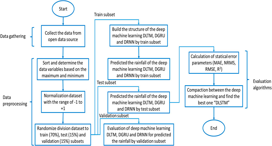
Figure 1. Flow chart diagram for the prediction of rainfall using DL models, highlighting data preprocessing, model training, and evaluation stages.

Where X_norm is the normalized variable value, x_min and x_max are the minimum and maximum variable values, respectively, and i represents the value for each data point.

The preprocessed data is then divided into three subsets: training set (70%), test set (15%), and validation set (15%). The training set is used to train the deep learning models, the test set is used to evaluate the performance of the models, and the validation set is used to adjust the parameters of the models. Next, three different deep learning models are built for rainfall predicting: DLSTM, DGRU, and DRNN. The DLSTM, DGRU, and DRNN models are trained using the training set, during which the models’ parameters are adjusted to learn the patterns in the training data. The performance of these models is then evaluated using the test set and validation set with metrics such as Root-Mean-Square Errors (RMSE), Normalized Root-Mean-Square Errors (NRMSE), Mean Absolute Errors (MAE), and Correction Coefficient (R²). Based on the evaluation results, the best deep learning model is selected for rain predicting; in this study, the DLSTM model was chosen as the best. The selected DLSTM model is then used for rain predicting, and the predict results are compared with the actual rainfall values. The study concludes that deep learning models can predict rainfall with high accuracy, with the DLSTM model identified as the most effective in this study.

2.2 Predicting using time series

Frequently, time series datasets, pertinent in predicting weather, monitoring stock market trends, and analyzing energy consumption patterns, manifest a fundamental trait: the sequentiality of time. Acknowledged as one of the top ten formidable tasks in data mining, owing to its inherent complexities, the quest for a robust model capable of discerning patterns within time series datasets persists as a important and arduous endeavor (Li et al., 2019).

Time series prediction can be classified as either a classification or regression problem. Typically, a series of data collected within a specific time frame is considered as the input for these problems. These details illustrate the progression of the phenomena (Equation 2).

$X=\left(X_1,X_2,\dots ,X_T\right)(2)$

Is a random variable and we have (Equation 3).

$X_T=\left(X_t^1,X_t^2,\dots ,X_t^L\right),X_t\in X(3)$

Where t represents time and L represents the length of the time step. Typically, past values are also given (Equation 4):

$y=\left(y_1,y_2,\dots ,y_{T-1}\right)(4)$

In classification problems, the historical values of the dependent variable, y, may vary. When the random variable X is confined to one dimension, solely a solitary characteristic is used in crafting the time series model from the diverse attributes characterizing a phenomenon. This model is denoted as “univariate.” Conversely, if multiple features are harnessed in crafting a time series model, it assumes the nomenclature of a “multivariate” time series model.

To ascertain the value of T utilizing the following formula, the customary approach involves exploring a nonlinear mapping function of the variable X and its associated target value y (Equation 5):

${\mathrm{ў}}_{\mathrm{T}}=\mathrm{f}\left(\mathrm{X},\mathrm{y}\right)(5)$

2.3 DRNN model architecture

The DRNN represents a densely interconnected neural architecture that integrates the temporal dimension into its structure. Diverging from conventional feed-forward networks, DRNNs incorporate feedback connections, facilitating the incorporation of both present and recent past information into the data processing framework (Lukoševičius and Jaeger, 2009; Fabbri and Moro, 2018; Sheng et al., 2023b). Through this distinctive architecture, DRNNs possess the capability to unveil correlations among events occurring across multiple temporal intervals, capturing enduring dependencies stemming from past occurrences (Wang et al., 2018; Song et al., 2020).

Nonetheless, akin to numerous neural network models, RNNs grapple with a pervasive performance obstacle referred to as the vanishing gradient problem. Throughout the learning phase, the gradient—a important indicator dictating weight adjustments based on errors—tends to either escalate excessively (resulting in an exploding gradient) or diminish significantly (leading to a vanishing gradient) (Lukoševičius and Jaeger, 2009; Neftci et al., 2019). This scenario complicates the training process, as precise gradient information is indispensable for accurate weight updates. To mitigate the vanishing gradient predicament, a variant of RNNs known as Long Short-Term Memory (LSTM) units is frequently used (Fei and Tan, 2018). LSTM units adeptly tackle this challenge by preserving error information as it traverses through time and layers. These units are specifically engineered to grasp long-term dependencies and mitigate issues associated with gradient instability.

LSTM units introduce a memory cell, comprising four primary components: an input gate, a self-recurrent connection, a forget gate, and an output gate (Gers et al., 2000; Chen et al., 2016). These gates play a pivotal role in regulating the information flow within the LSTM unit, facilitating decisions pertaining to data storage, retrieval, and modification (Zhang et al., 2021). In contrast to conventional recurrent neurons, LSTM units integrate these gates as innovative elements, effectively curbing gradient divergence.

For an exhaustive comprehension of DRNNs, LSTM units, and the mathematical formulations governing output evaluation and training, please consult the references provided (Alzubaidi et al., 2021). The hidden layer formulation for DRNN is delineated in Equation 6. The proposed architecture, depicted in Figure 2, exemplifies the typical functionality of DRNNs.

$R_t=\mathrm{f}\left({\mathrm{V}}_x,{\mathrm{W}}_{R\left(t-1\right)},b_R\right)(6)$

Figure 2

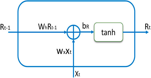
Figure 2. DRNN architecture for predicting rainfall: detailed schematic representation of the connections, and data flow within the network.

2.4 Deep Gated Recurrent Unit (DGRU) model architecture

The DGRUs represent specialized derivatives of Deep Recurrent Neural Networks (DRNNs) that have garnered significant attention in the domain of DLs. Rooted in the architecture of LSTM models, GRUs introduce a distinctive refinement in the form of an update gate integrated within their structure (Zhang et al., 2018). This update gate amalgamates the functionalities of both an input gate and a forget gate, rendering DGRUs potent instruments for sequence modeling.

The primary impetus driving the development of GRUs is to streamline the complexity of LSTM architectures while preserving their efficacy in capturing prolonged dependencies within sequential data (Campos et al., 2017; Che et al., 2018). By integrating an update gate, DGRUs strike a delicate equilibrium between assimilating pertinent information from the past and selectively disregarding superfluous data (Garcia-Garcia et al., 2017). This adaptive gating mechanism empowers GRUs to adeptly process sequential data and render precise predictions.

The configuration of a DGRU, as illustrated in Figure 3, delineates its internal constituents and the flow of information. It encompasses recurrent connections that facilitate information persistence across the sequence, encompassing an update gate, a reset gate, and a candidate activation function (Zulqarnain et al., 2020). These elements synergistically regulate information flow and update the hidden state of the DGRU at each time step.

Figure 3

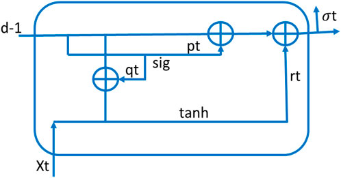
Figure 3. DGRU architecture for predicting rainfall: detailed schematic representation of the connections, and data flow within the network.

For a deeper comprehension of DGRU functionality, let us delve into the equations governing their operations (Hupkes et al., 2018). Equations 7-9 delineate the computational procedures intrinsic to GRUs. These equations elucidate how the update gate, reset gate, and candidate activation function interact with the current input, previous hidden state, and output of the GRU at each time step (Dey and Salem, 2017). By adjusting the weights and biases within these equations, GRUs can learn to model complex sequential patterns and make accurate predictions based on the given input data.

$\left\{\begin{array}{c}{p}_t=\mathrm{\sigma }\left({\mathrm{W}}_x\left[d_{t-1},x_t\right]+x_t\right)\\ q_t=\mathrm{\sigma }\left({\mathrm{W}}_x\left[d_{t-1},x_t\right]\right)\\ r_t=\tanh \left(\mathrm{W}\left[q_t\times d_{t-1},x_t\right]\right)\\ d_t=\left(1-p_t\right)\times d_{t-1}+p_t\times r_t\end{array}\right.(7)$

$\mathrm{\sigma }=\frac{1}{1+e^{-t}}(8)$

$\tanh \left(t\right)=\frac{1-e^{-2t}}{1+e^{-2t}}(9)$

2.5 Deep Long Short-Term Memory (DLSTM) model architecture

The DLSTM, pioneered by Hochreiter and Schmidhuber, represents a substantial enhancement to DRNN performance (Hochreiter and Schmidhuber, 1997). This variant of RNN, known as LSTM, leverages an DLSTM memory cell to encapsulate Long-Term Dependencies (LTD) within time series data. Additionally, in addressing the imperative of preserving long-term dependencies, DLSTM emerges as indispensable for mitigating the vanishing gradient issue inherent in DRNNs (Bengio et al., 1994; Sagheer and Kotb, 2019). The pivotal distinction between DLSTM and traditional DRNN cells resides in the mechanism used for activation computation. The DLSTM uses four distinct gates—namely the input gate, forget gate, output gate, and cell gate—to ascertain activation at time step t (Fang and Yuan, 2019).

The following relationship calculates the input of the information gate (in step t) (Equation 10):

$i_t=\sigma \left(W_{ia}.h_{t-1}+W_{ix}.x_i\right)(10)$

Where is a sigmoid-like non-linear function. Wia and W_ix are matrices that connect h (t-1) with h_t and x_t with h_t, respectively. The forget gate and output gate calculate their inputs as follows (Equations 11-12).

$f_t=\sigma \left(W_{ia}.h_{t-1}+W_{fx}.x_i\right)(11)$

$o_t=\sigma \left(W_{oa}.h_{t-1}+W_{ox}.x_i\right)(12)$

This is how the cell gate input is calculated (Equation 13):

$c_t=f_t.c_{t-1}+i_t.k_t(13)$

Where K_t is determined as follows, and C_t-1 represents the cell status data from the preceding phase (Equation 14):

$k_t=\tanh \left(w_{ca}.h_{t-1}+w_{cx}.x_t\right)(14)$

While using the tanh hyperbolic tangent function. Ultimately, the following formula is used to calculate the activation at step t (Equation 15):

$h_t=w_{ca}.\tanh \left(C_t\right)$

Enhancing the overall performance of a neural network commonly involves increasing its depth (Sagheer and Kotb, 2019). Illustrated in Figure 4, the DLSTM model amalgamates the benefits of a single DLSTM layer by sequentially connecting numerous DLSTM blocks in a recurrent network fashion. The overarching objective of stacking multiple DLSTMs within this hierarchical framework is to extract features in the lower layers that discern the sources of variation within the input data and subsequently amalgamate these representations in the upper layers (Sagheer and Kotb, 2019). Despite the fact that a deep architecture presents a more streamlined representation compared to a shallow one, empirical evidence has shown that deeper architectures tend to generalize more effectively, particularly for extensive or intricate datasets (Hermans and Schrauwen, 2013; Längkvist et al., 2014; Li et al., 2019). The parameters employed in the proposed model are delineated in Table 1.

Figure 4

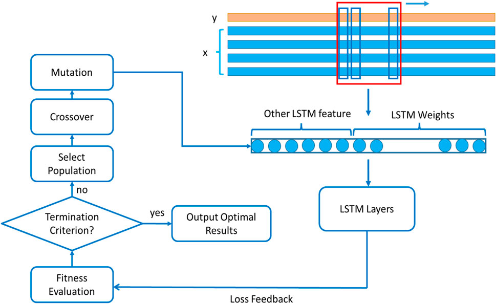
Figure 4. DLSTM architecture for predicting rainfall: detailed schematic representation of the connections, and data flow within the network.

Table 1

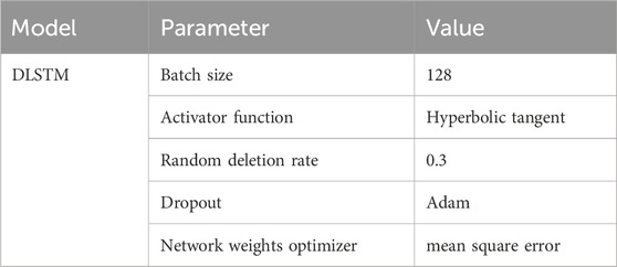
Table 1. Hyper parameters used in the DLSTM model, including activation functions, dropout rates, and other model’s performance.

One advantage of the stack architecture is that each layer accomplishes a part of the process before passing it on to the following layer, ultimately producing the final output. Another benefit of such systems is that they allow hidden states to operate across various time scales. The use of data with LTD or multivariate series data sets greatly benefits from these two advantages (Spiegel et al., 2011; Li et al., 2019). Figure 4, show DLSTM network architecture for prediction of rainfall. The process begins with a Select Population step, indicating that the model works with a population of potential DLSTM models. It then moves to a Fitness Evaluation step, assessing each model’s performance on a specific task, such as predicting the next word in a sequence. The flowchart then branches based on whether a Termination Criterion is met, which could be a set number of iterations or a desired performance level. If not met, the model proceeds to a Selection step, where the fittest models are chosen to be parents for the next-generation. This is followed by a Crossover step, where the genetic material (weights and biases) of two parent models is combined to create offspring. Optionally, a Mutation step introduces randomness by changing some weights or biases, preventing the model from getting stuck in local optima. The offspring are then evaluated for fitness, and the process repeats until the termination criterion is met. Finally, the flowchart concludes with an Output Optimal LSTM Layers step, indicating that the output is a set of weights and biases defining an optimal LSTM model for the task.

2.6 Cross validation evaluation

One superior technique for result validation is k-fold cross-validation. In this method, the entire dataset is considered a complete set, and DL models are applied. The data is then divided into two groups: test and train. Initially, one portion of the data is designated as the test subset, while the remaining portion serves as the training subset (Figure 5) (Bengio and Grandvalet, 2003; Al-Mudhafar, 2016). Subsequently, the roles are reversed, with the other portion of the data becoming the test set. This process is repeated for each of the k folds, with k set to 8 in this study. The entire procedure is conducted 10 times, resulting in an average of 80 iterations.

Figure 5

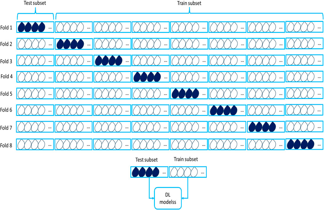
Figure 5. Detailed architecture of K-fold cross validation: methodology and process of iterative test/train divisions.

This validation approach effectively addresses analytical issues, enhancing result reliability while mitigating problems related to overfitting and model inefficiency in prediction. In this method, one batch is designated as the test subset, and the remaining seven batches are treated as the training set. Ultimately, the lowest average value from the data is considered the measure of prediction accuracy. This iterative process significantly contributes to result validation and ensures the robustness of the outcomes.

3 Data collection

To evaluate the effectiveness of the proposed models, a dataset comprising 12,852 data points collected from three cities in Indonesia: Kuantan, Butterworth, and Kuching, was utilized. This dataset consisted of weather information sourced from the Global Weather Data, spanning the period between 1797 and 2014. The data was obtained online from the website https://globalweather.tamu.edu. Leveraging this comprehensive and extensive weather dataset, researchers rigorously analyzed and validated the proposed models. The inclusion of such a substantial dataset enhances the credibility and robustness of the findings, ensuring that the models are well-suited for handling weather-related data within the specified time range.

Table 1 displays the statistical parameters for the range of data used in this study. For the prediction of rainfall, the models used several input variables, including maximum temperature (°C), minimum temperature (°C), wind speed (m/s), relative humidity (%), and solar radiation (MJ/m²). The statistical values of input and output data for rainfall prediction are reported in Table 2. According to the information presented, the maximum temperature ranges from −4.95°C to 27.97°C, the minimum temperature falls between −22.70°C and 15.36°C, the wind speed variable ranges from 0.66 m/s to 11.39 m/s, the relative humidity variable falls between 0.41 and 1.01, the solar radiation ranges from 0.19 MJ/m² to 35.24 MJ/m², and the rainfall output parameter falls between 0.00 mm and 69.80 mm.

Table 2

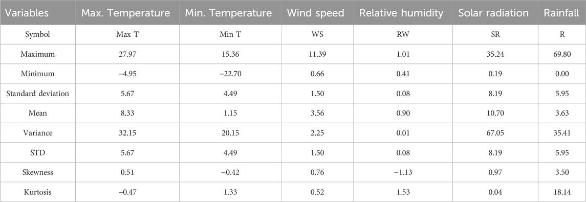
Table 2. Statistical parameters for the prediction of rainfall based on various input variables.

4 Discussion of results

4.1 Evaluation criteria

The statistical parameters for evaluation, including RMSE, NRMSE, MAE, and R², have previously been used as evaluation criteria for performance. These metrics are derived from Equations 16-19.

$MAE=\sqrt{\frac{1}{N}{\displaystyle \sum _{i=1}^N}\left[{\widehat{y}}_t^i-y_t^i\right]}(16)$

$RMSE=\sqrt{\frac{1}{N}{\displaystyle \sum _{i=1}^N}{\left({\widehat{y}}_t^i-y_t^i\right)}^2}(17)$

$NRMSE=\sqrt{\frac{1}{N}{\displaystyle \sum _{i=1}^N}\frac{{\left({\widehat{y}}_t^i-y_t^i\right)}^2}{\max \left(y_t\right)-\min \left(y_t\right)}}(18)$

${\mathrm{R}}^2=1-\frac{{\displaystyle \sum _{\mathrm{i}=1}^{\mathrm{N}}}{\left({\widehat{y}}_t^i-y_t^i\right)}^2}{{\displaystyle \sum _{\mathrm{i}=1}^{\mathrm{N}}}{\left(y_t^i-\frac{{\sum }_{\mathrm{I}=1}^{\mathrm{n}}{\widehat{y}}_t^i}{\mathrm{n}}\right)}^2}(19)$

Where; ${\widehat{y}}_t^i$ is the real value, $y_t^i$ is the predicted value, y_t is the vector of actual values, and N is the total number of test samples.

The details of the dataset and the procedure for partitioning it into training and test sets are visually depicted. The data allocation was carried out meticulously, with 70% assigned for training, 15% for validation, and the remaining 15% reserved for the test set for each meteorological dataset.

For an effective comparison of DL models, researchers can examine the statistical error parameters described in Equations 17-21, serving as quantitative measures of model performance. Table 3 provides a comprehensive overview of error values associated with various stages of rainfall prediction, including training, testing, validation, and the overall prediction. Analyzing the error values in the table allows researchers to gain insights into the accuracy and efficacy of the models in predicting rainfall. This evaluation aids in identifying models with lower error rates and provides valuable information for selecting the most suitable model for accurate rainfall prediction. The incorporation of statistical error parameters and the corresponding table enhances the scientific rigor and reliability of the comparative analysis.

Table 3

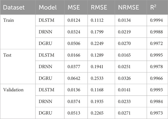
Table 3. Statistical results for rainfall prediction using DL models: performance metrics and comparative analysis.

Using the data outlined in Table 3 and the insights from Figure 6, a Cross-plot illustration for predicting rainfall through DL models, several noteworthy observations emerge. The mentioned figure represents the accuracy levels achieved by these models, serving as a visual depiction of their performance. Specifically, the figure effectively illustrates the discrepancy between the cross-plot line and the predicted data points.

Figure 6

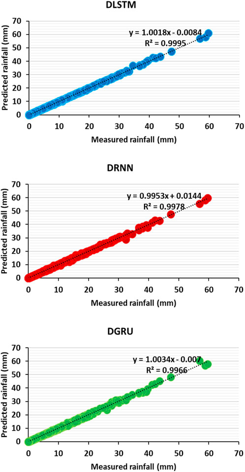
Figure 6. Cross plot illustration for prediction of rainfall in the test subset using DL models: a comparative analysis of model performance and accuracy.

Upon careful analysis of this figure alongside the results presented in Table 3, a clear pattern emerges, indicating that the accuracy of the DLSTM model surpasses that of both the DRNN and DGRU models. The evidence from the figure, coupled with the quantified outcomes in Table 3, unmistakably illustrates the superior precision and predictive capability exhibited by the DLSTM model.

Therefore, based on these results, it can be confidently stated that the DLSTM model outperforms its counterparts, namely, the DRNN and DGRU models, in terms of accuracy. These compelling results further emphasize the effectiveness and potential of DL models, specifically underscoring the prominence of DLSTM as a formidable tool for rainfall prediction.

Figure 7 serves as a significant visual representation of the error analysis conducted on the test sample data for rainfall prediction using DL models. This figure provides valuable insights into the calculation errors associated with the DLSTM, DRNN, and DGRU models.

Figure 7

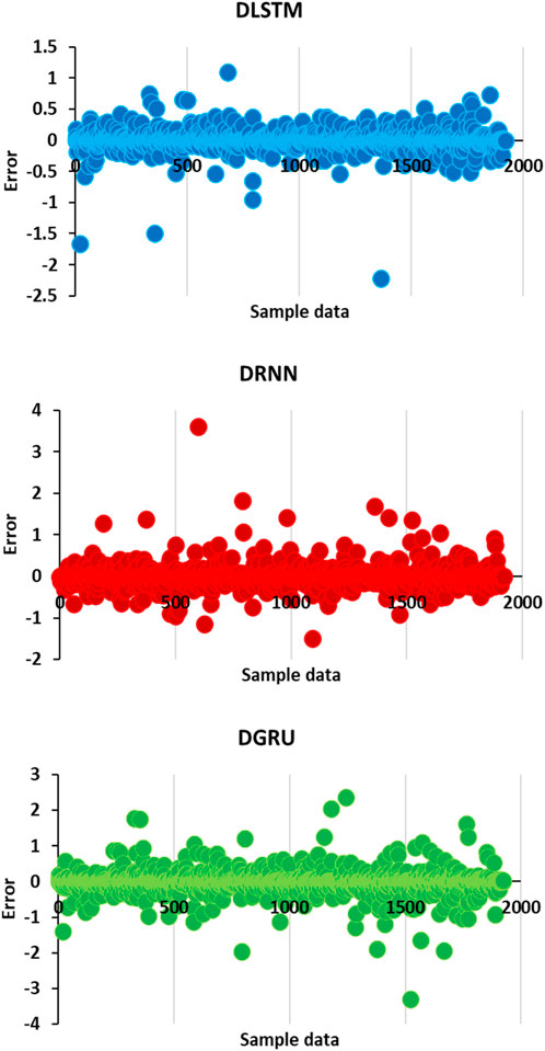
Figure 7. Error illustration for the test subset in predicting rainfall using DL models: a comparative analysis of model performance and error distributions.

Upon careful examination of this figure, it becomes evident that the calculation error for the DLSTM model is substantially lower than that of the DRNN and DGRU models. The calculated errors for DLSTM range between −1 and +1, indicating a remarkably narrow margin of deviation from the actual values. Conversely, the DRNN model exhibits a wider range of errors, spanning from −3 to +3, suggesting a comparatively higher level of inconsistency in its predictions. Similarly, the DGRU model displays an even larger range of errors, fluctuating between −6 and +6, thereby implying a greater degree of imprecision.

Based on the results presented in Figure 7, it is irrefutable that the calculation error rankings for the models used in this study follow the sequence: DLSTM > DRNN > DGRU. In other words, the DLSTM model exhibits the lowest calculation error, followed by the DRNN model, while the DGRU model yields the highest calculation error. These findings further reinforce the superior performance and accuracy of the DLSTM model compared to other models, emphasize its potential as a robust tool for precise rainfall prediction.

To visually assess the performance of DL models in predicting rainfall, the Regression Error Characteristics (REC) curve and the Area Over the Curve (AOC) value were used. The REC curve depicts the error distribution of predictive models by plotting error tolerance against the percentage of predictions falling within that tolerance. The AOC measures model accuracy, with a smaller AOC indicating superior performance. The REC method, indicating accuracy by showcasing the distribution of absolute deviation, serves as a measure to gauge performance accuracy. In AOC analysis, a higher value signifies lower model accuracy, while a lower value indicates higher accuracy (Azam et al., 2022). Figures 8, 9 present the REC curve and AOC curve for the test subset in predicting rainfall using DL models, respectively. Figure 8 clearly illustrates that the DLSTM model outperforms other DL models (DRNN and DGRU) in terms of performance accuracy. Figure 9 depicts the AOC value for the REC curve, with the highest value observed for the DGRU model and the lowest for the DLSTM model. Analyzing these figures leads to the conclusion that the DLSTM model exhibits the highest performance accuracy, while the DGRU model demonstrates the lowest.

Figure 8

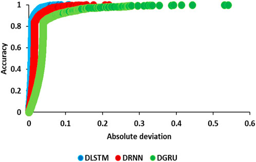
Figure 8. Illustration of the REC curve for the test subset in predicting rainfall using DL models: performance evaluation and comparison across different algorithms.

Figure 9

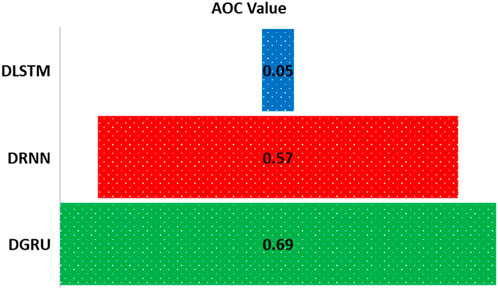
Figure 9. Illustration of AOC based on the REC curve for the test subset in predicting rainfall using DL models, highlighting model performance and accuracy.

Figure 10 presents a visual representation of the RMSE and R² parameters in the context of rainfall prediction using DL models. The graph showcases the performance of three models: DLSTM, DRNN, and DGRU, by evaluating the error values derived from the RMSE and R² metrics. Upon analyzing the graphical results, it becomes evident that the DLSTM model exhibits superior accuracy and performance compared to the other models. The figure provides valuable insights into the comparative effectiveness of these models in accurately predicting rainfall, highlighting DLSTM as the most accurate and reliable option among the three.

Figure 10

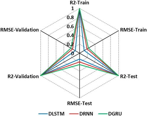
Figure 10. Graphical illustration of RMSE and R² parameters for evaluating the performance of deep learning models in predicting rainfall.

Figure 11 shows the histogram of predict errors for rainfall using three models: DLSTM, DRNN, and DGRU. Each histogram depicts the rainfall predict error for an model, displaying a normal distribution of predict errors centered around the zero axis, with a relatively narrow range and no detectable positive or negative bias. This graph enables a comprehensive analysis of the models’ performance and facilitates the identification of the model with the best performance based on its normal error distribution. After thorough examination, it becomes clear that the DLSTM model’s error distribution is more normal compared to the other models, indicating a superior and more accurate standard deviation. According to the comparison of these models based on the information presented in Table 3 and Figure 11, the performance accuracy of the models can be ranked as follows: DLSTM > DRNN > DGRU.

Figure 11

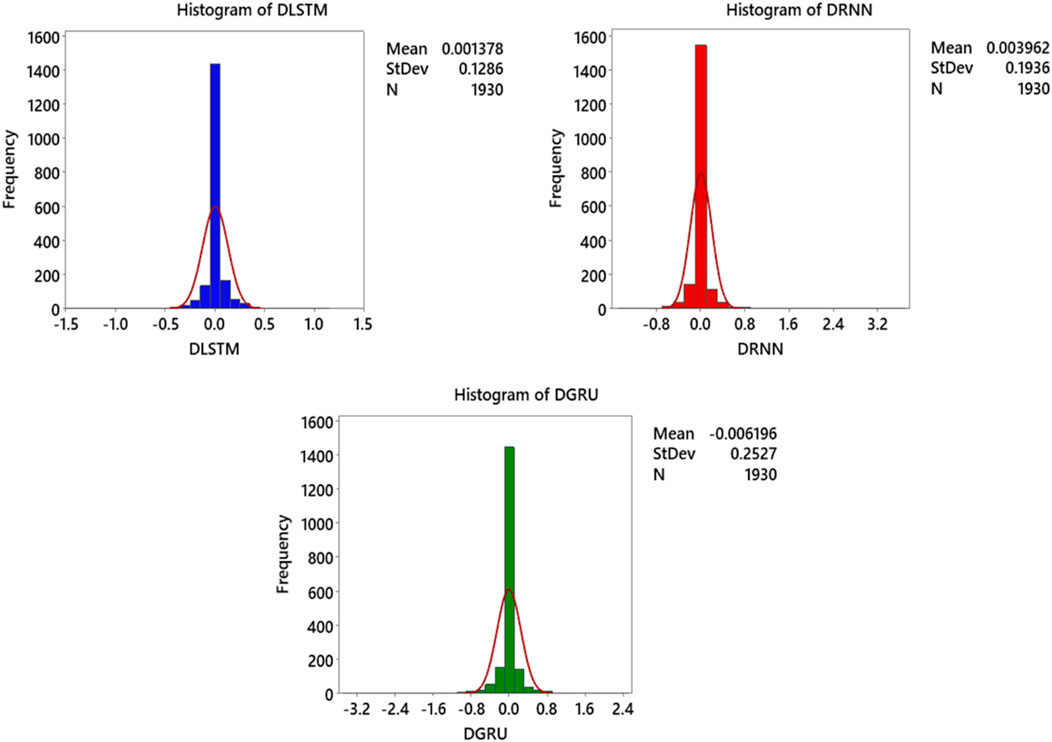
Figure 11. Histogram illustrating the distribution of prediction errors for rainfall forecasts by DL models, based on the test subset of the dataset.

Figure 12 show the graphical representation of error versus iteration for DLSTM, DRNN, and DGRU models. The graph provides valuable insights into the performance of these models over multiple iterations. Upon analyzing the figure, several observations can be made. Firstly, for the DLSTM model, it is evident that the error significantly decreases at iteration = 12, indicating a substantial reduction in error. Additionally, at iteration = 85, the quantitative error further diminishes, surpassing the error values of the other two models. Comparatively, the DGRU model showcases a reduction in error at iteration = 11, and a similar trend can be observed at iteration = 85. However, for the DRNN model, the error steadily decreases without any sudden fluctuations. Ultimately, at iteration = 100, the error comparison reveals that the DGRU model exhibits the highest error value among the three models, followed by DRNN and DLSTM, with DLSTM demonstrating the lowest error magnitude. This graphical representation allows for a comprehensive understanding of the error performance across different iterations, aiding in the evaluation and selection of the most effective DL models.

Figure 12

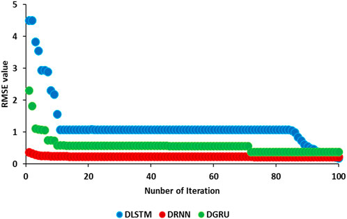
Figure 12. Illustration of error reduction versus iteration for DLSTM, DRNN, and DGRU models.

One method for evaluating models is through "score analysis.” This approach assigns a score to each statistical parameter, facilitating a comprehensive comparison among models. In this method, scores are determined by evaluating each model against a statistical error parameter, with the highest possible score being 9 and the lowest score being 1 for this study. Figure 13 illustrates the Score Analysis for the prediction and comparison of DLSTM, DRNN, and DGRU models. According to this figure, the Score Analysis values for LSTM, DRNN, and DGRU are 82, 66, and 31, respectively. This indicates that, based on the analysis, DLSTM outperforms DRNN, which in turn outperforms DGRU.

Figure 13

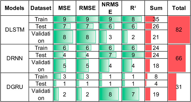
Figure 13. Graphical illustration for determination of score analysis in predicting rainfall using DL models.

Figure 14 displays the Taylor diagram used to evaluate the performance of DL models in predicting rainfall. In this diagram, the horizontal axis represents the standard deviation, which ranges from 0 to 0.3 in this study. A value closer to 1 indicates higher model accuracy. Additionally, the diagram shows the values of RMSE and R² as indicated by the radius of the circles. Points that are closer to the center of the quarter circle signify lower RMSE values, which correspond to improved model accuracy. As illustrated, the DLSTM model, with R2 = 0.9995, R² = 0.9995 and a standard deviation of 0.1285, demonstrates superior performance compared to the other models used for rainfall prediction.

Figure 14

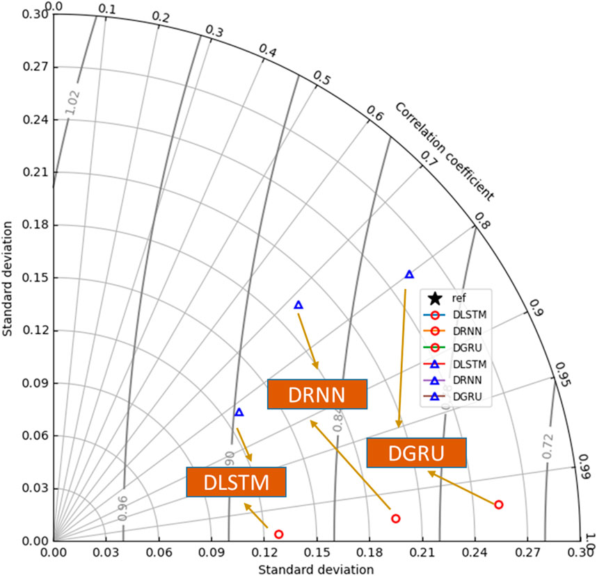
Figure 14. Graphical illustration of a Tylor diagram showing the prediction accuracy of rainfall using DL models, based on the test subset data.

To assess the influence of each input variable on rainfall, Spearman’s non-parametric correlation coefficient (R) is used. This coefficient ranges from −1 (indicating a complete negative correlation) to +1 (indicating a complete positive correlation), reflecting the variable’s impact as either low or high. The equation for Spearman’s coefficient is defined in Equation 20. The heat map graph is a valuable tool for analyzing changes in dependent and continuous variables. It visually represents the relationships between different parameters and helps determine the impact of input variables on the output parameter.

$R=\frac{{\displaystyle \sum _{i=1}^n}\left[\left(S_i-\overline{S}\right)\left(Q_i-\overline{Q}\right)\right]}{\sqrt{{\displaystyle \sum _{i=1}^n}{\left(S_i-\overline{S}\right)}^2}\sqrt{{\displaystyle \sum _{i=1}^n}{\left(Q_i-\overline{Q}\right)}^2}}(20)$

As shown in Figure 15, the maximum temperature and solar radiation parameters exhibit an indirect influence on the output parameter, while the minimum temperature, wind speed, and relative humidity parameters have a direct relationship with rainfall, as demonstrated by Equation 21.

$R\propto \frac{1}{\left(\mathit{Max}.T\&SR\right)},R\propto \left(\mathit{Min}.T\&WS\&RW\right)(21)$

Figure 15

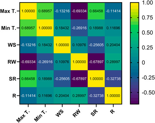
Figure 15. Heat map illustration of predicted rainfall based on input/output variables analysis.

5 Conclusion

In conclusion, this study highlights the critical role of rainfall in sustaining the water cycle and ecosystems, emphasizing the necessity for accurate predictions given the complex interactions between atmospheric and oceanic phenomena in today’s climate. Using 12,852 data points from open-source global weather data for three Indonesian cities, the study incorporated variables such as maximum and minimum temperatures, wind speed, relative humidity, and solar radiation to predict rainfall. Three advanced Deep Learning models—Recurrent Neural Network (DRNN), Deep Gated Recurrent Unit (DGRU), and Deep Long Short-Term Memory (DLSTM)—were employed, with the DLSTM model demonstrating superior performance, achieving Root-Mean-Square Errors (RMSE) and Correction Coefficient (R²) values of 0.1289 and 0.9995, respectively. The DLSTM model’s ability to handle long-term dependencies and its memory cell architecture with forget gates enable it to retain and retrieve important information, making it particularly effective for time series predictions. Additionally, its parallelization capabilities enhance computational efficiency, while its flexibility in model design and regularization techniques improve generalization performance. The study also found that maximum temperature and solar radiation have an indirect influence on rainfall, whereas minimum temperature, wind speed, and relative humidity directly affect it. Overall, the DLSTM model’s superior performance in capturing complex weather patterns and delivering high-precision rainfall predictions underscores its value in meteorological data analysis and forecasting, surpassing the capabilities of DRNN and DGRU models. DLSTM networks excel in rainfall prediction by capturing long-term dependencies, handling temporal variability, and modeling non-linear relationships between meteorological variables. They manage complex atmospheric interactions, handle missing data robustly, and adapt to changing weather patterns effectively.

Data availability statement

The data analyzed in this study is subject to the following licenses/restrictions: The datasets will available with the corresponding authors due to reasonable academic’s request. Requests to access these datasets should be directed to HGH; hamzehghorbani68@yahoo.com.

Author contributions

HL: Conceptualization, Data curation, Methodology, Project administration, Resources, Writing–original draft, Writing–review and editing. SL: Conceptualization, Data curation, Funding acquisition, Methodology, Project administration, Resources, Writing–original draft, Writing–review and editing. HGH: Conceptualization, Data curation, Methodology, Resources, Software, Supervision, Visualization, Writing–original draft, Writing–review and editing.

Funding

The author(s) declare that no financial support was received for the research, authorship, and/or publication of this article.

Acknowledgments

The project of young backbone teachers in Henan Province colleges and universities (2021GGJS182): Research on control system of intelligent fruit picking robot based on binocular vision; A series of research-oriented teaching projects in Henan province: A typical case of cultivating innovative talents in undergraduate colleges and universities (46).

Conflict of interest

The authors declare that the research was conducted in the absence of any commercial or financial relationships that could be construed as a potential conflict of interest.

Publisher’s note

All claims expressed in this article are solely those of the authors and do not necessarily represent those of their affiliated organizations, or those of the publisher, the editors and the reviewers. Any product that may be evaluated in this article, or claim that may be made by its manufacturer, is not guaranteed or endorsed by the publisher.

Supplementary material

The Supplementary Material for this article can be found online at: https://www.frontiersin.org/articles/10.3389/fenvs.2024.1445967/full#supplementary-material

References

Akhtar, M., Shatat, A. S. A., Ahamad, S. A. H., Dilshad, S., and Samdani, F. (2023). Optimized cascaded CNN for intelligent rainfall prediction model: a research towards statistic-based machine learning. Theor. Issues Ergonomics Sci. 24 (5), 564–592. doi:10.1080/1463922x.2022.2135786

CrossRef Full Text | Google Scholar

Al-Mudhafar, W. J. (2016). Incorporation of bootstrapping and cross-validation for efficient multivariate facies and petrophysical modeling. Denver, CO: SPE. SPE-180277.

Google Scholar

Alzubaidi, L., Zhang, J., Humaidi, A. J., Al-Dujaili, A., Duan, Y., Al-Shamma, O., et al. (2021). Review of deep learning: concepts, CNN architectures, challenges, applications, future directions. J. Big Data 8, 53–74. doi:10.1186/s40537-021-00444-8

PubMed Abstract | CrossRef Full Text | Google Scholar

Azam, A., Bardhan, A., Kaloop, M. R., Samui, P., Alanazi, F., Alzara, M., et al. (2022). Modeling resilient modulus of subgrade soils using LSSVM optimized with swarm intelligence algorithms. Sci. Rep. 12 (1), 14454. doi:10.1038/s41598-022-17429-z

PubMed Abstract | CrossRef Full Text | Google Scholar

Baljon, M., and Sharma, S. K. (2023). Rainfall prediction rate in Saudi Arabia using improved machine learning techniques. Water 15 (4), 826. doi:10.3390/w15040826

CrossRef Full Text | Google Scholar

Bengio, Y., and Grandvalet, Y. (2003). No unbiased estimator of the variance of k-fold cross-validation. Adv. Neural Inf. Process. Syst. 16.

Google Scholar

Bengio, Y., Simard, P., and Frasconi, P. (1994). Learning long-term dependencies with gradient descent is difficult. IEEE Trans. Neural Netw. 5 (2), 157–166. doi:10.1109/72.279181

PubMed Abstract | CrossRef Full Text | Google Scholar

Beniston, M. (2003). Climatic change in mountain regions: a review of possible impacts. Clim. Change 59 (1), 5–31. doi:10.1007/978-94-015-1252-7_2

CrossRef Full Text | Google Scholar

Campos, V., Jou, B., Giró-i-Nieto, X., Torres, J., and Chang, S.-F. (2017). Skip rnn: learning to skip state updates in recurrent neural networks. arXiv Prepr. arXiv, 170806834. doi:10.48550/arXiv.1708.06834

CrossRef Full Text | Google Scholar

Chang, N.-B., Yang, Y. J., Imen, S., and Mullon, L. (2017). Multi-scale quantitative precipitation forecasting using nonlinear and nonstationary teleconnection signals and artificial neural network models. J. Hydrology 548, 305–321. doi:10.1016/j.jhydrol.2017.03.003

PubMed Abstract | CrossRef Full Text | Google Scholar

Che, Z., Purushotham, S., Cho, K., Sontag, D., and Liu, Y. (2018). Recurrent neural networks for multivariate time series with missing values. Sci. Rep. 8 (1), 6085. doi:10.1038/s41598-018-24271-9

PubMed Abstract | CrossRef Full Text | Google Scholar

Chen, Y., Zhong, K., Zhang, J., Sun, Q., and Zhao, X. (2016). LSTM networks for mobile human activity recognition. Atlantis Press, 50–53. doi:10.2991/icaita-16.2016.13

CrossRef Full Text | Google Scholar

DelSole, T., and Shukla, J. (2002). Linear prediction of Indian monsoon rainfall. J. Clim. 15 (24), 3645–3658. doi:10.1175/1520-0442(2002)015<3645:lpoimr>2.0.co;2

CrossRef Full Text | Google Scholar

Deo, R. C., and Şahin, M. (2015). Application of the extreme learning machine algorithm for the prediction of monthly Effective Drought Index in eastern Australia. Atmos. Res. 153, 512–525. doi:10.1016/j.atmosres.2014.10.016

CrossRef Full Text | Google Scholar

Dey, R., and Salem, F. M. (2017). Gate-variants of gated recurrent unit (GRU) neural networks. IEEE, 1597–1600. doi:10.1109/MWSCAS.2017.8053243

CrossRef Full Text | Google Scholar

Dwivedi, D. K., Kelaiya, J. H., and Sharma, G. R. (2019). Forecasting monthly rainfall using autoregressive integrated moving average model (ARIMA) and artificial neural network (ANN) model: a case study of Junagadh, Gujarat, India. J. Appl. Nat. Sci. 11 (1), 35–41. doi:10.31018/jans.v11i1.1951

CrossRef Full Text | Google Scholar

Fabbri, M., and Moro, G. (2018). Dow jones trading with deep learning: the unreasonable effectiveness of recurrent. Neural Netw. 142–153. doi:10.5220/0006922101420153

CrossRef Full Text | Google Scholar

Fahad, S., Su, F., Khan, S. U., Naeem, M. R., and Wei, K. (2023). Implementing a novel deep learning technique for rainfall forecasting via climatic variables: an approach via hierarchical clustering analysis. Sci. Total Environ. 854, 158760. doi:10.1016/j.scitotenv.2022.158760

PubMed Abstract | CrossRef Full Text | Google Scholar

Fang, X., and Yuan, Z. (2019). Performance enhancing techniques for deep learning models in time series forecasting. Eng. Appl. Artif. Intell. 85, 533–542. doi:10.1016/j.engappai.2019.07.011

CrossRef Full Text | Google Scholar

Fei, H., and Tan, F. (2018). Bidirectional grid long short-term memory (bigridlstm): a method to address context-sensitivity and vanishing gradient. Algorithms 11 (11), 172. doi:10.3390/a11110172

CrossRef Full Text | Google Scholar

Garcia-Garcia, A., Orts-Escolano, S., Oprea, S., Villena-Martinez, V., and Garcia-Rodriguez, J. (2017). A review on deep learning techniques applied to semantic segmentation. arXiv Prepr. arXiv, 170406857. doi:10.48550/arXiv.1704.06857

CrossRef Full Text | Google Scholar

Gers, F. A., Schmidhuber, J., and Cummins, F. (2000). Learning to forget: continual prediction with LSTM. Neural Comput. 12 (10), 2451–2471. doi:10.1162/089976600300015015

PubMed Abstract | CrossRef Full Text | Google Scholar

Goutham, N., Alonzo, B., Dupré, A., Plougonven, R., Doctors, R., Liao, L., et al. (2021). Using machine-learning methods to improve surface wind speed from the outputs of a numerical weather prediction model. Boundary-Layer Meteorol. 179, 133–161. doi:10.1007/s10546-020-00586-x

CrossRef Full Text | Google Scholar

He, R., Zhang, L., and Chew, A. W. Z. (2022). Modeling and predicting rainfall time series using seasonal-trend decomposition and machine learning. Knowledge-Based Syst. 251, 109125. doi:10.1016/j.knosys.2022.109125

CrossRef Full Text | Google Scholar

Hermans, M., and Schrauwen, B. (2013). Training and analysing deep recurrent neural networks. Adv. Neural Inf. Process. Syst. 26.

Google Scholar

Hochreiter, S., and Schmidhuber, J. (1997). Long short-term memory. Neural Comput. 9 (8), 1735–1780. doi:10.1162/neco.1997.9.8.1735

PubMed Abstract | CrossRef Full Text | Google Scholar

Hupkes, D., Veldhoen, S., and Zuidema, W. (2018). Visualisation and 'diagnostic classifiers' reveal how recurrent and recursive neural networks process hierarchical structure. J. Artif. Intell. Res. 61, 907–926. doi:10.1613/jair.1.11196

CrossRef Full Text | Google Scholar

Knight, C., and Washington, R. (2024). Remote midlatitude control of rainfall onset at the southern African tropical edge. J. Clim. 37, 2519–2539. doi:10.1175/jcli-d-23-0446.1

CrossRef Full Text | Google Scholar

Kumar, V., Kedam, N., Sharma, K. V., Khedher, K. M., and Alluqmani, A. E. (2023). A comparison of machine learning models for predicting rainfall in urban metropolitan cities. Sustainability 15 (18), 13724. doi:10.3390/su151813724

CrossRef Full Text | Google Scholar

Längkvist, M., Karlsson, L., and Loutfi, A. (2014). A review of unsupervised feature learning and deep learning for time-series modeling. Pattern Recognit. Lett. 42, 11–24. doi:10.1016/j.patrec.2014.01.008

CrossRef Full Text | Google Scholar

Latif, S. D., Hazrin, N. A. B., Koo, C. H., Ng, J. L., Chaplot, B., Huang, Y. F., et al. (2023). Assessing rainfall prediction models: exploring the advantages of machine learning and remote sensing approaches. Alexandria Eng. J. 82, 16–25. doi:10.1016/j.aej.2023.09.060

CrossRef Full Text | Google Scholar

Latif, S. D., Mohammed, D. O., and Jaafar, A. (2024). Developing an innovative machine learning model for rainfall prediction in a semi-arid region. J. Hydroinformatics 26 (4), 904–914. doi:10.2166/hydro.2024.014

CrossRef Full Text | Google Scholar

Li, Y., Zhu, Z., Kong, D., Han, H., and Zhao, Y. (2019). EA-LSTM: evolutionary attention-based LSTM for time series prediction. Knowledge-Based Syst. 181, 104785. doi:10.1016/j.knosys.2019.05.028

CrossRef Full Text | Google Scholar

Lukoševičius, M., and Jaeger, H. (2009). Reservoir computing approaches to recurrent neural network training. Comput. Sci. Rev. 3 (3), 127–149. doi:10.1016/j.cosrev.2009.03.005

CrossRef Full Text | Google Scholar

Markuna, S., Kumar, P., Ali, R., Vishwkarma, D. K., Kushwaha, K. S., Kumar, R., et al. (2023). Application of innovative machine learning techniques for long-term rainfall prediction. Pure Appl. Geophys. 180 (1), 335–363. doi:10.1007/s00024-022-03189-4

CrossRef Full Text | Google Scholar

Neftci, E. O., Mostafa, H., and Zenke, F. (2019). Surrogate gradient learning in spiking neural networks: bringing the power of gradient-based optimization to spiking neural networks. IEEE Signal Process. Mag. 36 (6), 51–63. doi:10.1109/msp.2019.2931595

CrossRef Full Text | Google Scholar

Nicholson, S. E. (2017). Climate and climatic variability of rainfall over eastern Africa. Rev. Geophys. 55 (3), 590–635. doi:10.1002/2016rg000544

CrossRef Full Text | Google Scholar

Norel, M., Kałczyński, M., Pińskwar, I., Krawiec, K., and Kundzewicz, Z. W. (2021). Climate variability indices—a guided tour. Geosciences 11 (3), 128. doi:10.3390/geosciences11030128

CrossRef Full Text | Google Scholar

Pham, B. T., Le, L. M., Le, T.-T., Bui, K.-T. T., Le, V. M., Ly, H.-B., et al. (2020). Development of advanced artificial intelligence models for daily rainfall prediction. Atmos. Res. 237, 104845. doi:10.1016/j.atmosres.2020.104845

CrossRef Full Text | Google Scholar

Sagheer, A., and Kotb, M. (2019). Time series forecasting of petroleum production using deep LSTM recurrent networks. Neurocomputing 323, 203–213. doi:10.1016/j.neucom.2018.09.082

CrossRef Full Text | Google Scholar

Saleh, M. A., Rasel, H. M., and Ray, B. (2024). A comprehensive review towards resilient rainfall forecasting models using artificial intelligence techniques. Green Technol. Sustain. 2, 100104. doi:10.1016/j.grets.2024.100104

CrossRef Full Text | Google Scholar

Sheng, Z., Wen, S., Feng, Z.-k, Gong, J., Shi, K., Guo, Z., et al. (2023b). A survey on data-driven runoff forecasting models based on neural networks. IEEE Trans. Emerg. Top. Comput. Intell. 7 (4), 1083–1097. doi:10.1109/tetci.2023.3259434

CrossRef Full Text | Google Scholar

Sheng, Z., Wen, S., Feng, Z.-K., Shi, K., and Huang, T. (2023a). A novel residual gated recurrent unit framework for runoff forecasting. IEEE Internet Things J. 10 (14), 12736–12748. doi:10.1109/jiot.2023.3254051

CrossRef Full Text | Google Scholar

Song, T., Ding, W., Liu, H., Wu, J., Zhou, H., and Chu, J. (2020). Uncertainty quantification in machine learning modeling for multi-step time series forecasting: example of recurrent neural networks in discharge simulations. Water 12 (3), 912. doi:10.3390/w12030912

CrossRef Full Text | Google Scholar

Spiegel, S., Gaebler, J., Lommatzsch, A., De Luca, E., and Albayrak, S. (2011). Pattern recognition and classification for multivariate time series, 34–42.

Google Scholar

Tricha, A., and Moussaid, L. (2024). Evaluating machine learning models for precipitation prediction in Casablanca City. Indonesian J. Electr. Eng. Comput. Sci. 35 (2), 1325–1332. doi:10.11591/ijeecs.v35.i2.pp1325-1332

CrossRef Full Text | Google Scholar

Wang, H., Xie, K., Lian, Z., Cui, Y., Chen, Y., Zhang, J., et al. (2018). Large-scale circuitry interactions upon earthquake experiences revealed by recurrent neural networks. IEEE Trans. Neural Syst. Rehabilitation Eng. 26 (11), 2115–2125. doi:10.1109/tnsre.2018.2872919

PubMed Abstract | CrossRef Full Text | Google Scholar

Zhang, C., Sheng, Z., Zhang, C., and Wen, S. (2024). Multi-lead-time short-term runoff forecasting based on ensemble attention temporal convolutional network. Expert Syst. Appl. 243, 122935. doi:10.1016/j.eswa.2023.122935

CrossRef Full Text | Google Scholar

Zhang, L., Wang, S., and Liu, B. (2018). Deep learning for sentiment analysis: a survey. Wiley Interdiscip. Rev. Data Min. Knowl. Discov. 8 (4), e1253. doi:10.1002/widm.1253

CrossRef Full Text | Google Scholar

Zhang, X., Liu, L., Long, G., Jiang, J., and Liu, S. (2021). Episodic memory governs choices: an rnn-based reinforcement learning model for decision-making task. Neural Netw. 134, 1–10. doi:10.1016/j.neunet.2020.11.003

PubMed Abstract | CrossRef Full Text | Google Scholar

Zulqarnain, M., Abd, I. S., Ghazali, R., Nawi, N. M., Aamir, M., and Hassim, Y. M. M. (2020). An improved deep learning approach based on variant two-state gated recurrent unit and word embeddings for sentiment classification. Int. J. Adv. Comput. Sci. Appl. 11 (1). doi:10.14569/ijacsa.2020.0110174

CrossRef Full Text | Google Scholar

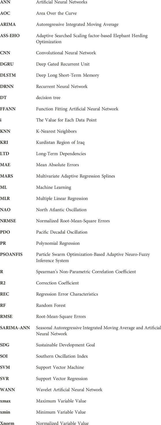
Nomenclature