Innovation and application of inter-provincial carbon emission transfer accounting model in China’s domestic production network

The New Development Paradigm will result in the significant development of domestic production networks and the accelerated growth of carbon transfers among provinces in China. However, the existing value chain or the trade of intermediate goods decomposition method cannot completely account for the carbon content of intermediate goods. So the paper developed a accounting model for inter-regional intermediate goods trade based on input-output model. The most significant advantage of this accounting model is that by further decomposing final output into three components—final consumption within the region, final consumption flowing to other regions, and final output flowing to other regions as intermediate goods that are not returned to the region—it achieves a more comprehensive decomposition of the value chain in comparison to the established models. This approach allows for the tracking of longer value chains and the accounting for intermediate goods inflows and outflows simultaneously. Furthermore, the accounting of trade in intermediate goods can be conducted for any number of countries, regions, and sectors within the input-output system, thereby providing a foundation for the comprehensive accounting of inter-regional carbon transfers within production networks. With the input-output tables and carbon emission inventories from the CEADs (the China Carbon Emissions Accounting Database), the paper has calculated the changes of the carbon transfer among provinces in the China’s domestic production network from 2012 to 2017 and find that the inter-provincial intermediate goods trade and carbon transfer among provinces is increasing significantly. Each province has a strong incentive to overuse the carbon embodied in the intermediate goods from others, but lacks the motivation to reduce their own carbon emission. In the inter-provincial transfer of the carbon content of intermediate goods in China’s domestic production network, the difference between the average value of the ratio of the carbon content of intermediate goods from other provinces used by each province and that supplied for use by other provinces to the ratio of the carbon content of intermediate goods produced by itself increased by 13.6% between 2012 and 2017. Only a few provinces are evolving towards a win-win between economic and environmental benefits, while most are still facing the evolutionary dilemma in choosing between economic and environmental benefits. In the future, we should comprehensively explore the cooperative governance of carbon emission reduction in the domestic production network, including establishing a national standard for calculating the carbon transfer in domestic production network, improving the carbon emission responsibility sharing mechanism and carbon emission reduction compensation systems.

1 Introduction

In order to achieve the goal of carbon peaking and carbon neutrality, every region and key emitting enterprise in China has formulated a carbon emission reduction strategy. In addition, a number of local carbon emissions trading markets have also been established (GUO-Song and DUAN, 2024). By the end of 2023, a total of 440 million tonnes of carbon credits had been traded, resulting in approximately RMB 2.49 billion in trade value (Pan, 2024). Furthermore, the recently revised Interim Regulations on the Administration of Carbon Emissions Trading had been implemented on 1 May 2024. In the future, the accurate calculation of inter-regional carbon transfers and the fair distribution of carbon allowances will be of paramount importance in advancing the construction of a unified national carbon emissions trading market. However, all of this is predicated on an accurate accounting of inter-regional, inter-sector and inter-company carbon emission responsibilities.

The initial calculation for carbon emission responsibility was conducted either from the consumer principle or the producer principle and mostly based on input-output models. First, in the context of multilateral trade, Peters et al. (2011) found that in the majority of developed countries, consumption-based emissions have increased at a faster rate than territorial emissions, the transfer of emissions is largely attributed to non-energy-intensive manufacturing, the role of international trade in explaining changes in emissions in many countries is significant, both in terms of production and consumption. Davis and Caldeira (2010) presented a global consumption-based CO₂ emissions inventory and calculations of associated consumption-based energy and carbon intensities. Their findings indicate that wealthy countries are net importers of carbon emissions while developing and emerging market countries are generally net exporters of carbon emissions. An environmentally extended multi-region input-output model was employed by Wang et al. (2018) to track India’s CO₂ emission streams through international supply chains from primary emitters to final producers to final consumers, and found that both production-based and consumption-based emissions have exhibited a constant growth trajectory from 2000 to 2014. However, production-based emissions demonstrated higher growth rates. The principal recipients of India’s export emissions are developed countries, whereas the principal sources of India’s import emissions are developing countries. Furthermore, intermediate goods are the primary contributors to both export and import emissions. The evolution of CO₂ emissions embodied in international trade in Poland was analyzed by Tsagkari et al. (2018) using the Input-Output method, specifically by constructing a multi-regional input-output model and found that Poland is a net importer of carbon emissions from other European countries with less strict environmental policies. Weber and Matthews (2007) employed a multi-country input-output model of the United States and its seven largest trading partners to analyse the environmental impacts of changes in the structure and volume of U.S. trade from 1997 to 2004, and found that augmented imports and shifts in trade patterns have resulted in considerable increases in U.S. embodied emissions of carbon dioxide, sulfur dioxide, and nitrogen oxides from trade. Second, in the context of bilateral trade, Wang et al. (2015) has also made a significant contribution. They have extended the decomposition of a country’s total trade flows proposed by Koopman et al. (2014) to studies at the sector, bilateral, and bi-sector levels, the international trade flows at all levels are decomposed into the components of value-added exports, returned domestic value-added, foreign value-added, and purely double-counted trade in intermediates, and are further distinguished into 16 different paths according to the source of the value of the traded goods, the final place of absorption, and the channels of absorption, thus a systematic correspondence between international trade statistics and the System of National Economic Accounts (SNA) has been established. The study also made a further contribution to methodological changes in the separation of carbon content of trade in intermediate goods from that of aggregate trade. Other authors who have made scholarly contributions to the field include: Du et al. (2011) employed an input-output analysis based on the energy/dollar ratio (EDR) to estimate the embodied carbon emissions from U.S.-China trade. Additionally, a structural decomposition analysis (SDA) is utilised to examine the underlying drivers of changes in China’s embodied carbon emissions from exports to the U.S. over the period 2002–2007. Yu and Chen (2017) employed an input-output model to calculate and decompose the embodied carbon emissions associated with trade between China and South Korea from 2000 to 2010, and to identify the underlying causes of observed changes. Long et al. (2018) utilized a multi-region input-output model and incorporated the rest of the world as a benchmark to analyse the difference of the direct and complete carbon dioxide emissions intensity and economic activities of China and Japan. Yu et al. (2023) established inter-sector linkages based on the global value chain framework and utilized the Asian Development Bank’s International Input-Output Database (IIOD) to investigate the influence of supply and demand dynamics and wealth accumulation on China’s carbon emissions within the context of inter-regional trade between China and the Association of Southeast Asian Nations (ASEAN). Wang et al. (2022) empirically analyzed the relationship between the GVC embedded position and the environmental dividend under the construction of “Belt and Road” trade corridors in China. Based on the WIOD database, Yue and Yun-long, 2019 presented an empirical investigation of the impact of China’s global value chains on carbon emissions. Based on the input-output data and carbon emission data released by China’s Carbon Accounting Databases (CEADs), Wang (2022) presented innovatively a carbon emission responsibility sharing mechanism under the “beneficiary principle” and a carbon emission reduction technology compensation mechanism under the “counterfactual condition”.

It is worth noting that some of the existing studies on accounting for carbon responsibility with input-output model shows a significant difference between the results of accounting following the consumer principle and that of accounting following the producer principle (Peng et al., 2015; Li et al., 2020). As a result, they have been heavily critiqued. (Peters, 2008; Peters et al., 2011; Peng et al., 2015; 2016). This difference can be attributed to the fact that embedded carbon transfers from trade in intermediate goods in production networks are not accounted for separately. Instead, they are either simply allocated to the first producer (producer principle) or to the last consumer (consumer principle). It is essential to distinguish the accounting of the transfer of carbon content of intermediate goods trade from that of volume trade in production networks (Peng et al., 2016).

In addition to this, there are two other types of literature that provide valuable references for research on accounting for carbon emissions responsibilities. The first is the evaluation of embedded carbon over the entire life cycle, such as Du et al. (2024), Tian et al. (2024), Wang et al. (2023), Hong-ran et al. (2024), Lu and Wang (2024). The second is the investigation of the structural characteristics of multi-regional carbon emission networks and their evolution, such as Song et al. (2024), Jie et al. (2024), Yang (2022), Xiao-Yu et al. (2024), Ji et al. (2023), Gan and Wang (2022), and Yang et al. (2024). However, these two strands of literature still do not consider the issue of inter-regional, inter-sector, and inter-firm transfers of carbon content of intermediate goods trade.

In summary, the accounting of embedded carbon transfers in intermediate goods in production networks necessitates the utilization of intermediate goods trade model. The degree of completeness of the decomposition of intermediate goods flows by the intermediate goods trade model determines the degree of accuracy in accounting for the carbon content of intermediate goods trade in the production network. Up to now, there are two mathematically equivalent models of trade in intermediate goods (Wu, 2019), they are Koopman et al. (2014) and Wang et al. (2015), respectively. Those two models completely decompose the international or inter-regional flows of intermediate goods and their embedded factors on the basis of destination and use and then already form the theoretical basis of the methodology for accounting for carbon content of intermediate goods trade. Specifically, Koopman et al. (2014) developed a three-country model that can decompose a country’s total exports into 9 indicators based on the flow of value added from the country, presenting one of the earliest methods of completely decomposing a country’s exports. Subsequently, Wang et al. (2015) further proposed a three-country model that can decompose a country’s exports into 16 indicators based on Koopman et al. (2014). Later, Los et al. (2016) further simplified the decomposition result of Koopman et al. (2014) using hypothetical extraction. Muradow (2016) further refined the decomposition result of Wang et al. (2015) into 8 indicators. However, the shortcomings of these two models are as follows: first, the models are unsuitable for tracking intermediate goods trade in longer value chains. Second, they cannot calculate the carbon content of the intermediate goods trade from both import and export directions simultaneously. Third, their decomposition items are too complex to analyse.

So this paper will apply the block matrix to the Leontief inverse matrix to establish a comprehensive decomposition model for national or regional exports that can be applied to any number of regions, any length of the value chain, and can simultaneously account for the real value of imports (inflows) and exports (outflows) of intermediate goods for a given region. The innovation of this paper with respect to the decomposition model of trade in intermediate goods will provide a theoretical basis for completely accounting for the carbon content of inter-provincial intermediate goods trade in China. The most significant advantage of the accounting model is that by further decomposing final output of a given region into three components—final consumption within the region, final consumption flowing to other regions, and final output flowing to other regions as intermediate goods that are not returned to the region—it could achieve a more comprehensive decomposition of the value chain in comparison to these established models. The possible marginal contribution of this article is shown in the following: first, exploring the accounting model of complete (i.e., not merely direct) carbon transfer among regions within a domestic production network. Second, research on inter-provincial transfer of carbon content of inter-provincial intermediate goods trade from a domestic production network perspective has not been found in the literature as far as the authors’ reading is concerned. Third, the analysis also encompasses the carbon demand and supply behaviour, as well as the net carbon supply, of the 31 provinces within the aforementioned domestic production network. Fourth, the model built in the paper can facilitate a comprehensive understanding of the carbon reduction strategies employed by each of these provinces in their domestic production networks.

2 Methods and data

2.1 Accounting for inter-provincial intermediate goods trade in domestic production networks

Conventionally, the matrix of input-output coefficients is represented as A, the vector of total output as X, and the vector of final consumption as Y. According to input-output theory, the following Equation 1 holds true in multi-regional input-output model (MRIO):

$\mathit{A}\mathit{X}+\mathit{Y}=\mathit{X}(1)$

The multi-regional input-output table includes 31 provinces and 42 industries, set $n=\left[1,2,\dots \dots ,31\right]$, $m=\left[1,2,\dots \dots ,42\right]$. Thus, 961 block matrices are included in $A_{nn}$, and each block matrix has another 1764 elements $a_{mm}^{\prime }$. Namely Equation 2:

${\mathit{A}}_{\mathit{n}\mathit{n}}=\left[\begin{array}{ccc}{\mathit{A}}_{\mathbf{11}}& \cdots & {\mathit{A}}_{\mathbf{1}\mathit{n}}\\ ⋮& \ddots & ⋮\\ {\mathit{A}}_{\mathit{n}\mathbf{1}}& \cdots & {\mathit{A}}_{\mathit{n}\mathit{n}}\end{array}\right]\to {\mathit{a}}_{\mathit{m}\mathit{m}}=\left[\begin{array}{ccc}{\mathit{a}}_{\mathbf{11}}& \cdots & {\mathit{a}}_{\mathbf{1}\mathit{m}}\\ ⋮& \ddots & ⋮\\ {\mathit{a}}_{\mathit{m}\mathbf{1}}& \cdots & {\mathit{a}}_{\mathit{m}\mathit{m}}\end{array}\right](2)$

The total output vector $X$ consists of 31 block column vectors $X_n$, and each block column vector contains the total output vector of 42 industries $X_m$. Namely Equation 3:

${\mathit{X}}_{\mathit{n}}=\left[\begin{array}{c}{\mathbf{X}}_{\mathbf{1}}\\ ⋮\\ {\mathbf{X}}_{\mathbf{n}}\end{array}\right]\to {\mathit{x}}_{\mathit{n}}=\left[\begin{array}{c}{\mathit{x}}_{\mathbf{1}}\\ ⋮\\ {\mathit{x}}_{\mathit{m}}\end{array}\right](3)$

The final consumption matrix $Y$ consists of 961 block matrices $Y_{nn}$, each $y_{nn}$ containing 1764 elements. Namely:

$Y_{\mathit{nn}}=\left[\begin{array}{ccc}{Y}_{11}& \cdots & Y_{1n}\\ ⋮& \ddots & ⋮\\ Y_{n1}& \cdots & Y_{\mathit{nn}}\end{array}\right]\to y_{\mathit{mm}}=\left[\begin{array}{ccc}{y}_{11}& \cdots & y_{1m}\\ ⋮& \ddots & ⋮\\ y_{m1}& \cdots & y_{\mathit{mm}}\end{array}\right](4)$

The final consumption matrix $Y_{nn}$ and its block matrix $Y_{mm}$ can be divided into two parts: (1) the final output for final consumption in this province, denoted as $Y_{nn}$; (2) the final output for final consumption in other provinces, denoted as $Y_{n\overline{n}}$ ($n+\overline{n}=31$). In Equation 4, the elements on the main diagonal of $Y_{nn}$, and its block matrix $y_{mm}$ represent the final output produced in the region for its own consumption, and the other elements off the main diagonal represent the final output produced in the region for consumption in other regions. Furthermore, the final output of the region is not only used by the final consumption of the region and other regions, but also a part can be used by other regions as intermediate goods in the production of final consumption goods, and will not return to the region in the form of intermediate goods, denoted as ${\mathit{Int}}_{n\overline{n}}$. Therefore, the final output of a given province $n$ can be expressed as:

${\mathit{F}\mathit{O}}_{\mathit{n}}=\left[{\mathit{Y}}_{\mathit{n}\mathit{n}}{\mathit{Y}}_{\mathit{n}\overline{\mathit{n}}}+{\mathit{Int}}_{\mathit{n}\overline{\mathit{n}}}\right](5)$

Furthermore, in the context of the inter-provincial intermediate goods trade, the sum of final goods consumption, the sum of final goods output and the sum of total output of each province satisfy the following relationship: ${\sum }_n{Y}_n<{\sum }_n{FO}_n<{\sum }_n{X}_n$. This provides a basis for expanding the accounting scope of the existing intermediate goods trade.

We will focus on the derivation of the accounting methods of the three target variables: (1) the complete demand of the province $n$ for intermediate goods from any other province $\overline{n}$, denoted as ${ITZ}_{\overline{n}\to n}$; (2) The complete demand of intermediate goods for its own in the province $n$ is denoted as ${DTZ}_{n\to n}$ ; (3) The complete demand of any other province $\overline{n}$ for intermediate goods in that province $n$ is denoted as ${ETZ}_{n\to \overline{n}}$.

(1) accounting ${ITZ}_{\overline{n}\to n}$, that is, the demand of province $n$ for intermediate goods from all other provinces $\overline{n}$. Obviously, ${ITZ}_{\overline{n}\to n}$ is derived from the need of the province $n$ to produce the final output ${FO}_n$. According to Equation 5, to further completely compute ${FO}_n$, it is necessary to solve the quantity of intermediate goods that flow to all other provinces $\overline{n}$ and no longer flow back to the province $n$ as intermediate goods, namely ${\mathit{Int}}_{n\overline{n}}$. For the same reason, the demand for intermediate goods of $n$ in all other provinces $\overline{n}$ is derived from the output level of final goods $Y_{\overline{n}}$, and it also has two purposes: one is for final consumption in the province $\overline{n}$, and the other is for final consumption in other provinces $n$, that is $Y_{\overline{n}}=\left[Y_{\overline{n}\overline{n}}{Y}_{\overline{n}n}\right]$, the demand for intermediate goods in other provinces is derived from the output level of final goods in other provinces. According to the input-output theory, the primary direct demand of provinces for intermediate products of other provinces is $A_{n\overline{n}}{Y}_{\overline{n}}$, the secondary indirect demand can be $A_{n\overline{n}}{A_{\overline{n}\overline{n}}Y}_{\overline{n}}$, and the third indirect demand is $A_{n\overline{n}}{A_{\overline{n}\overline{n}}^{2}Y}_{\overline{n}}$, and the fourth indirect demand is $A_{n\overline{n}}{A}_{\overline{n}\overline{n}}^3{Y}_{\overline{n}}$, and the nth indirect demand is $A_{n\overline{n}}{A}_{\overline{n}\overline{n}}^{n-1}{Y}_{\overline{n}}$. The complete demand of any other province $\overline{n}$ for intermediate goods of the province $n$ can be expressed as:

${\mathbf{Int}}_{\mathbf{n}\to \overline{\mathbf{n}}}={\mathbf{A}}_{\mathbf{n}\overline{\mathbf{n}}}\left({\mathbf{Y}}_{\overline{\mathbf{n}}\overline{\mathbf{n}}}+{\mathbf{Y}}_{\overline{\mathbf{n}}\mathbf{n}}\right)+{\mathbf{A}}_{\mathbf{n}\overline{\mathbf{n}}}{\mathbf{A}}_{\overline{\mathbf{n}}\overline{\mathbf{n}}}\left({\mathbf{Y}}_{\overline{\mathbf{n}}\overline{\mathbf{n}}}+{\mathbf{Y}}_{\overline{\mathbf{n}}\mathbf{n}}\right)+{\mathbf{A}}_{\mathbf{n}\overline{\mathbf{n}}}{\mathbf{A}}_{\overline{\mathbf{n}}\overline{\mathbf{n}}}^2\left({\mathbf{Y}}_{\overline{\mathbf{n}}\overline{\mathbf{n}}}+{\mathbf{Y}}_{\overline{\mathbf{n}}\mathbf{n}}\right)+\dots ={\mathbf{A}}_{\mathbf{n}\overline{\mathbf{n}}}{\left(\mathbf{I}-{\mathbf{A}}_{\overline{\mathbf{n}}\overline{\mathbf{n}}}\right)}^{-1}\left({\mathbf{Y}}_{\overline{\mathbf{n}}\overline{\mathbf{n}}}+{\mathbf{Y}}_{\overline{\mathbf{n}}\mathbf{n}}\right)$

Where, $\mathit{I}$ represents the identity matrix. Finally, ${\mathit{Int}}_{n\overline{n}}$ is substituted into Equation 5, and the complete expression of the final output of provinces $n$ is the following Equation 6:

${\mathit{F}\mathit{O}}_{\mathit{n}}=\left[{\mathit{Y}}_{\mathit{n}\mathit{n}}{\mathit{Y}}_{\mathit{n}\overline{\mathit{n}}}+{\mathit{A}}_{\mathit{n}\overline{\mathit{n}}}{\left(\mathit{I}-{\mathit{A}}_{\overline{\mathit{n}}\overline{\mathit{n}}}\right)}^{-\mathbf{1}}\left({\mathit{Y}}_{\overline{\mathit{n}}\overline{\mathit{n}}}+{\mathit{Y}}_{\overline{\mathit{n}}\mathit{n}}\right)\right](6)$

Next, we can use the final output ${FO}_n$ of the province $n$ to derive its actual demand $Z_{\overline{n}\to n}$ for intermediate goods from all other provinces $\overline{n}$. It is worth noting that the calculation results ${\mathit{Int}}_{n\to \overline{n}}$ derived above are based on the final output $Y_{\overline{n}}$ of the provinces $\overline{n}$ and only include two types of intermediate goods flowing from the provinces $n$ to the provinces $\overline{n}$: (1) the intermediate goods of the provinces $n$ needed to meet the production of the final goods used by the provinces $\overline{n}$ themselves, and (2) the intermediate goods of the provinces $n$ needed to meet the production of the final goods of any other province $n$. In other words, ${\mathit{Int}}_{n\to \overline{n}}$ does not include the quantity of intermediate goods needed to satisfy the production of intermediate goods in any other province $n$. Therefore, the actual demand of any province for intermediate goods from other provinces should be derived on the basis of the final output ${FO}_n$ of the province $n$, because it includes the final output of the province formed for the demand of intermediate goods from other regions to produce final output, and includes the flow of intermediate goods not included in ${\mathit{Int}}_{n\to \overline{n}}$. According to the input-output principle, the primary direct demand of the final output ${FO}_n$ of a province $\mathbf{n}$ for intermediate goods of any other province is denoted as $A_{\overline{n}n}{FO}_n$, the secondary indirect demand is denoted as $A_{\overline{n}n}{A_{\overline{n}\overline{n}}FO}_n$, and the third indirect demand is denoted as $A_{\overline{n}n}{A}_{\overline{n}\overline{n}}^2{FO}_n$, and the forth indirect demand is denoted as $A_{\overline{n}n}{A}_{\overline{n}\overline{n}}^3{FO}_n$, and the nth indirect demand is denoted as $A_{\overline{n}n}{A}_{\overline{n}\overline{n}}^{n-1}{FO}_n$. The actual demand of the intermediate goods of all other provinces derived from the final output ${FO}_n$ of a province $n$ can be expressed as the following Equation 7:

${\mathit{Z}}_{\overline{\mathit{n}}\to \mathit{n}}={\mathit{A}}_{\overline{\mathit{n}}\mathit{n}}{\mathit{F}\mathit{O}}_{\mathit{n}}+{\mathit{A}}_{\overline{\mathit{n}}\mathit{n}}{{\mathit{A}}_{\overline{\mathit{n}}\overline{\mathit{n}}}\mathit{F}\mathit{O}}_{\mathit{n}}+{\mathit{A}}_{\overline{\mathit{n}}\mathit{n}}{\mathit{A}}_{\overline{\mathit{n}}\overline{\mathit{n}}}^{\mathbf{2}}{\mathit{F}\mathit{O}}_{\mathit{n}}+\dots ={\mathit{A}}_{\overline{\mathit{n}}\mathit{n}}{\left(\mathit{I}-{\mathit{A}}_{\mathit{n}\mathit{n}}\right)}^{-\mathbf{1}}{\mathit{F}\mathit{O}}_{\mathit{n}}(7)$

Next, on the basis of $Z_{\overline{n}\to n}$, we need to further derive the complete demand of the intermediate goods by province $n$ for the all other provinces, marked as ${ITZ}_{\overline{n}\to n}$. According to the input-output principle, the inverse Leontief matrix is $L={\left(I-A\right)}^{-1}$, after shifting terms, we can obtain: $L\times \left(I-A\right)=I$. The minimalist block matrix is used to list the equivalence relation as follows:

$\left[\begin{array}{cc}{\mathit{L}}_{\mathit{n}\mathit{n}}& {\mathit{L}}_{\mathit{n}\overline{\mathit{n}}}\\ {\mathit{L}}_{\overline{\mathit{n}}\mathit{n}}& {\mathit{L}}_{\overline{\mathit{n}}\overline{\mathit{n}}}\end{array}\right]\left(\left[\begin{array}{cc}{\mathit{I}}_{\mathit{n}}& \mathbf{0}\\ \mathbf{0}& {\mathit{I}}_{\overline{\mathit{n}}}\end{array}\right]-\left[\begin{array}{cc}{\mathit{A}}_{\mathit{n}\mathit{n}}& {\mathit{A}}_{\mathit{n}\overline{\mathit{n}}}\\ {\mathit{A}}_{\overline{\mathit{n}}\mathit{n}}& {\mathit{A}}_{\overline{\mathit{n}}\overline{\mathit{n}}}\end{array}\right]\right)=\left[\begin{array}{cc}{\mathit{I}}_{\mathit{n}}& \mathbf{0}\\ \mathbf{0}& {\mathit{I}}_{\overline{\mathit{n}}}\end{array}\right](8)$

According to the relationship between these block matrices in the second row and the first column of Equation 8, it can be seen that: $L_{\overline{n}n}-\left(L_{\overline{n}n}{A}_{nn}+L_{\overline{n}\overline{n}}{A}_{\overline{n}n}\right)=0$. Through algebraic shift and necessary transformation, we can obtain: $L_{\overline{n}n}=L_{\overline{n}\overline{n}}{A}_{\overline{n}n}{\left({I-A}_{nn}\right)}^{-1}$. This is the coefficient matrix of the complete demand of one province for the intermediate goods of all other provinces, and then multiply ${FO}_n$ both sides by each other to obtain ${ETZ}_{\overline{n}\to n}$ which is the expression for the complete demand of the province $n$ for all intermediate goods of any other province:

${\mathit{I}\mathit{T}\mathit{Z}}_{\overline{\mathit{n}}\to \mathit{n}}={\mathit{L}}_{\overline{\mathit{n}}\mathit{n}}{\mathit{F}\mathit{O}}_{\mathit{n}}={\mathit{L}}_{\overline{\mathit{n}}\overline{\mathit{n}}}{\mathit{A}}_{\overline{\mathit{n}}\mathit{n}}{\left({\mathit{I}-\mathit{A}}_{\mathit{n}\mathit{n}}\right)}^{-1}{\mathit{F}\mathit{O}}_{\mathit{n}}\to {\mathit{I}\mathit{T}\mathit{Z}}_{\overline{\mathit{n}}\to \mathit{n}}={\mathit{L}}_{\overline{\mathit{n}}\overline{\mathit{n}}}{\mathit{Z}}_{\overline{\mathit{n}}\to \mathit{n}}(9)$

At this point, we have obtained the accounting method of the actual demand $Z_{\overline{n}\to n}$ and complete demand ${ITZ}_{\overline{n}\to n}$ of the intermediate goods for all other provinces $\overline{n}$ from the province $n$.

(2) accounting ${DTZ}_{n\to n}$, that is the provincial demand for its own intermediate goods. Since there is no flow of intermediate goods between provinces, according to the basic input-output principle, the complete demand of the final output of a province for its own intermediate goods will be reflected as the total output of the region, which is similar to Equation 9, namely the following Equation 10:

${{\mathit{D}\mathit{T}\mathit{Z}}_{\mathit{n}\to \mathit{n}}=\mathit{L}}_{\mathit{n}\mathit{n}}{\mathit{F}\mathit{O}}_{\mathit{n}}={\mathit{X}}_{\mathit{n}}(10)$

(3) accounting ${ETZ}_{n\to \overline{n}}$, that is the complete demand of any other province $\overline{n}$ for the intermediate goods of the province $n$. Similarly, according to the relationship of the block matrix in the first row and the second column in Equation 8, it can be known that: $L_{n\overline{n}}-\left(L_{nn}{A}_{n\overline{n}}+L_{n\overline{n}}{A}_{\overline{n}\overline{n}}\right)=0$. Through algebraic shift and necessary transformation, we can obtain: $L_{n\overline{n}}=L_{nn}{A}_{n\overline{n}}{\left(I-A_{\overline{n}\overline{n}}\right)}^{-1}$. By multiplying ${FO}_{\overline{n}}$ both sides of this equation, we can obtain the expression ${ETZ}_{n\to \overline{n}}$ of the complete supply of intermediate goods by the province $\mathrm{n}$ to all other provinces $\overline{n}$, namely the Equation 11:

${\mathit{E}\mathit{T}\mathit{Z}}_{\mathit{n}\to \overline{\mathit{n}}}={\mathit{L}}_{\mathit{n}\overline{\mathit{n}}}{\mathit{F}\mathit{O}}_{\overline{\mathit{n}}}={\mathit{L}}_{\mathit{n}\mathit{n}}{\mathit{A}}_{\mathit{n}\overline{\mathit{n}}}{\left(\mathit{I}-{\mathit{A}}_{\overline{\mathit{n}}\overline{\mathit{n}}}\right)}^{-\mathbf{1}}{\mathit{F}\mathit{O}}_{\overline{\mathit{n}}}(11)$

where ${FO}_{\overline{n}}=\left[Y_{\overline{n}\overline{n}}{Y}_{\overline{n}n}+A_{\overline{n}n}{\left(I-A_{nn}\right)}^{-1}\left(Y_{nn}+Y_{n\overline{n}}\right)\right]$. According to the input-output principle, there is the following relationship between the actual demand and complete demand of intermediate goods of province $n$ in any other province $\overline{n}$: $Z_{n\to \overline{n}}=A_{n\overline{n}}{\left(I-A_{\overline{n}\overline{n}}\right)}^{-1}{FO}_{\overline{n}}$. Obviously, the two equations, $L_{n\overline{n}}{FO}_{\overline{n}}$ and $L_{nn}{Z}_{n\to \overline{n}}$ , are mathematically equivalent and both are equal to the ${ETZ}_{n\to \overline{n}}$.

At this point, we have completed the derivation of the accounting methods for the three target variables of the province complete demand for its own intermediate goods, the complete demand for the intermediate goods of any other province, and the complete supply of the intermediate goods for any other province in the economic system. To sum up, if the inter-provincial trade of intermediate goods in any province is ${TOT}_n$, then we can get the following Expression 12:

${\mathit{T}\mathit{O}\mathit{T}}_{\mathit{n}}=\left[\begin{array}{c}{\mathit{I}\mathit{T}\mathit{Z}}_{\overline{\mathit{n}}\to \mathit{n}}\\ {\mathit{D}\mathit{T}\mathit{Z}}_{\mathit{n}\to \mathit{n}}\\ {\mathit{E}\mathit{T}\mathit{Z}}_{\mathit{n}\to \overline{\mathit{n}}}\end{array}\right]=\left[\begin{array}{c}{\mathit{L}}_{\overline{\mathit{n}}\mathit{n}}{\mathit{F}\mathit{O}}_{\mathit{n}}\\ {\mathit{L}}_{\mathit{n}\mathit{n}}{\mathit{F}\mathit{O}}_{\mathit{n}}\\ {\mathit{L}}_{\mathit{n}\overline{\mathit{n}}}{\mathit{F}\mathit{O}}_{\overline{\mathit{n}}}\end{array}\right](12)$

If the net supply of provincial participation in domestic inter-regional intermediate goods trade is ${NCE}_n$, its expression is as the following Equation 13:

${\mathit{N}\mathit{C}\mathit{E}}_{\mathit{n}}={\mathit{E}\mathit{T}\mathit{Z}}_{\mathit{n}\to \overline{\mathit{n}}}-{\mathit{I}\mathit{T}\mathit{Z}}_{\overline{\mathit{n}}\to \mathit{n}}(13)$

It is worth noting that we use the block matrix for the derivation of the target variable accounting method, but it does not imply a one-to-one correspondence between the direct consumption coefficient matrix and its Leontief inverse, i.e., $L_{nn}\ne {\left(I-A_{nn}\right)}^{-1}$.

2.2 Accounting for inter-provincial carbon transfers in China’s domestic production networks

In fact, as long as the inter-provincial intermediate goods trade model derived in this paper is combined with the CO₂ emission intensity at the provincial-industry level, the completely embodied carbon calculation model of domestic production network can be obtained. Where, the CO₂ emission intensity of any “provincial-industry” is represented by the CO₂ emissions per unit of added value of the “provincial-industry”. The CO₂ emission intensity of industry $m$ in province $n$ is denoted as ${CD}_{nm}$ and ${CD}_{nm}=\frac{{TCD}_{nm}}{{VAL}_{nm}}$. Where ${TCD}_{nm}$ and ${VAL}_{nm}$ represents the total volume of CO₂ emission and value-added of industry $m$ in province $n$. The diagonal matrix of CO₂ emission intensity is marked as $CD$, and its block matrix can be expressed as:

$\mathit{C}\mathit{D}=\left[\begin{array}{ccc}{\mathit{C}\mathit{D}}_{\mathbf{1}}& \cdots & \mathbf{0}\\ ⋮& \ddots & ⋮\\ \mathbf{0}& \cdots & {\mathit{C}\mathit{D}}_{\mathit{n}}\end{array}\right]$

Among them, each block matrix in $CD$ is a diagonal matrix containing the CO₂ emission intensity of 42 industries ${CD}_{nm}$. Further, if the carbon content of inter-provincial intermediate trade of a province $n$ is marked as ${CTOT}_n$, namely the following Equation 14:

${\mathit{C}\mathit{T}\mathit{O}\mathit{T}}_{\mathit{n}}=\left[\begin{array}{c}{\mathit{C}\mathit{I}\mathit{T}\mathit{Z}}_{\overline{\mathit{n}}\to \mathit{n}}\\ {\mathit{C}\mathit{D}\mathit{T}\mathit{Z}}_{\mathit{n}\to \mathit{n}}\\ \mathit{C}{\mathit{E}\mathit{T}\mathit{Z}}_{\mathit{n}\to \overline{\mathit{n}}}\end{array}\right]=\left[\begin{array}{l}{{\mathit{C}\mathit{D}}_{\overline{\mathit{n}}}\mathit{L}}_{\overline{\mathit{n}}\mathit{n}}{\mathit{F}\mathit{O}}_{\mathit{n}}\\ {\mathit{C}\mathit{D}}_{\mathit{n}}{\mathit{L}}_{\mathit{n}\mathit{n}}{\mathit{F}\mathit{O}}_{\mathit{n}}\\ {\mathit{C}\mathit{D}}_{\mathit{n}}{\mathit{L}}_{\mathit{n}\overline{\mathit{n}}}{\mathit{F}\mathit{O}}_{\overline{\mathit{n}}}\end{array}\right](14)$

Where, ${{CD}_{\overline{n}}L}_{\overline{n}n}{FO}_n$ represents the complete carbon content of the intermediate goods flowing into the province $n$ from other provinces $\overline{n}$ in China, ${CD}_n{L}_{nn}{FO}_n$ represents the complete carbon content of the inter-provincial intermediate goods trade between industries in the province $n$, and ${CD}_n{L}_{n\overline{n}}{FO}_{\overline{n}}$ represents the complete carbon content of intermediate goods flowing from the province $n$ to any other province $\overline{n}$. Similarly, the net outflow of carbon content of inter-provincial intermediate goods trade from province $n$ is expressed as the following Equation 15:

${\mathit{C}\mathit{N}\mathit{C}\mathit{E}}_{\mathit{n}}=\mathit{C}{\mathit{E}\mathit{T}\mathit{Z}}_{\mathit{n}\to \overline{\mathit{n}}}-\mathit{C}{\mathit{I}\mathit{T}\mathit{Z}}_{\overline{\mathit{n}}\to \mathit{n}}(15)$

2.3 Data

All data are from the China Carbon Emissions Accounting Database (CEADs). For more information on the data, please refer to these following literature: Shan et al. (2016), Shan et al. (2018); Shan et al. (2020), Guan (2021), Xu et al. (2024), Zheng, H. et al. (2021).

3 Results

3.1 Carbon demand and evolution of each province in China’s production network

We will use two key variables to describe the demand pattern of carbon content of inter-provincial intermediate goods trade in each province: (1) the proportion of carbon content of intermediate goods from other provinces in the total carbon content of intermediate goods in each province, i.e. ${\theta }_{\overline{n}\to n}={ITZ}_{\overline{n}\to n}/\left({ITZ}_{\overline{n}\to n}+{DTZ}_{\overline{n}\to n}\right)$; (2) The difference between the carbon emission intensity of intermediate goods produced in other provinces and those produced in the province, i.e. ${∆}_{\overline{n}\to n}={ITZ}_{\overline{n}\to n}/Z_{\overline{n}\to n}-{DTZ}_{n\to n}/X_n$. Figures 1, 2 depict the demand pattern for carbon content of intermediate goods in each province in 2012 and 2017, respectively. Among them, the horizontal axis represents the variable ${\theta }_{\overline{n}\to n}$ , and the national mean is set as the origin, and the vertical axis represents the variable ${∆}_{\overline{n}\to n}$. The unit of measurement for both the horizontal and vertical axes is percentage (%).

Figure 1

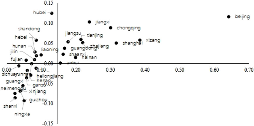
Figure 1. The Carbon Demand of Each Provinces: 2012, Notes: the horizontal axis represents the variable ${\theta }_{\overline{n}\to n}$, and the national mean is set as the origin, and the vertical axis represents the variable ${∆}_{\overline{n}\to n}$. They are all measured in percentage (%).

Figure 2

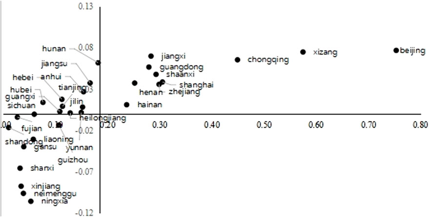
Figure 2. The Carbon Demand of Each Provinces: 2017. Notes: the horizontal axis represents the variable ${\theta }_{\overline{n}\to n}$, and the national mean is set as the origin, and the vertical axis represents the variable ${∆}_{\overline{n}\to n}$. They are all measured in percentage (%).

3.1.1 Carbon demand in each province

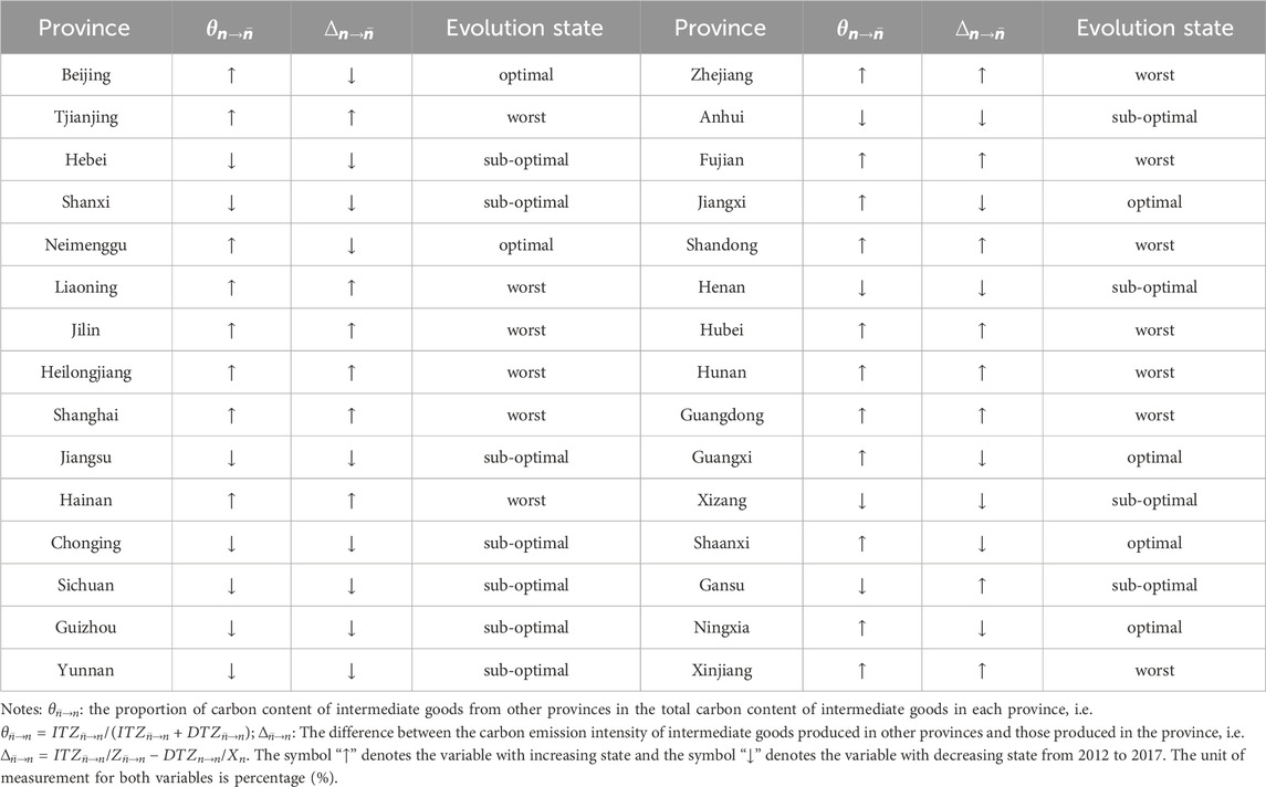
Figures 1, 2 depict the demand pattern for carbon content of intermediate goods in each province in 2012 and 2017 respectively. It is worth noting that for graphical display aesthetics, the value of ${\theta }_{\overline{n}\to n}$ and ${∆}_{\overline{n}\to n}$ in Qinghai is too large to be shown in the graph.

In the first quadrant, ${\theta }_{\overline{n}\to n}<\overline{\theta }$ and ${∆}_{\overline{n}\to n}>0$. Here, $\overline{\theta }$ is the average of $\theta$ in all provinces. Provinces located in the first quadrant have a lower percentage of carbon content in the intermediate goods they receive from other provinces, as compared to the national average. However, the carbon emission intensity of the intermediate goods received from other provinces is higher than their own. This indicates that these provinces can transfer some responsibility for carbon emissions to other provinces through the domestic production network. In 2012, seven provinces, including Hubei, Shandong, Hebei, Hunan, Liaoning, Jilin, and Fujian, adopted this carbon demand pattern. In 2017, there are still seven provinces followed this demand pattern, including Hunan, Jiangsu, Anhui, Hebei, Hubei, Tianjin, and Jilin. The number of provinces has remained the same since 2012, the newly added provinces are Jiangsu, Anhui, and Tianjin, while the removed provinces are Shandong, Liaoning, and Fujian.

In the second quadrant, ${\theta }_{\overline{n}\to n}>\overline{\theta }$ and ${∆}_{\overline{n}\to n}>0$. Provinces located in the second quadrant have a higher percentage of carbon content of the intermediate goods they receive from other provinces, compared to the national average. Additionally, the carbon emission intensity of the intermediate goods received from other provinces is also higher than their own. This means that these provinces have the strongest comparative advantage in transfer of the responsibility of carbon emissions to other provinces through the domestic production network. In 2012, eleven provinces followed the demand pattern of carbon in the domestic production network. Among them, Beijing has the strongest comparative advantage, followed by Jiangxi, Chongqing, and Tibet. The other seven provinces, including Shanghai, Tianjin, Zhejiang, Jiangsu, Guangdong, Shaanxi, and Hainan, are relatively weak. In 2017, ten provinces adopted the demand model of carbon in the domestic production network, including Beijing, Tibet, Chongqing, Jiangxi, Guangdong, Shaanxi, Shanghai, Zhejiang, Henan, and Hainan. Compared to 2012, the number of members increased by one and decreased by two. Henan was added, and Tianjin and Jiangsu were subtracted.

In the third quadrant, ${\theta }_{\overline{n}\to n}>\overline{\theta }\text{\hspace{0.17em}and\hspace{0.17em}}{∆}_{\overline{n}\to n}<0$. Provinces located in the third quadrant have a higher percentage of carbon they receive from other provinces than the national average. However, the carbon emission intensity of the intermediate goods received from other provinces is lower than their own. This means that these provinces cannot transfer the responsibility of carbon emissions to other provinces through the domestic production network. It's worth noting that no province followed this pattern of demand for carbon content of the inter-provincial intermediate goods trade in 2012 and 2017.

In the fourth quadrant, ${\theta }_{\overline{n}\to n}<\overline{\theta }$ and ${∆}_{\overline{n}\to n}<0$. Provinces located in the fourth quadrant have a lower percentage of carbon they receive from other provinces compared to the national average. Additionally, the carbon emission intensity of the intermediate goods they receive from other provinces is also lower than their own emission intensity. This indicates that these provinces cannot transfer the responsibility of carbon emissions to other provinces through the domestic production network. In 2012, ten provinces, including Heilongjiang, Henan, Yunnan, Gansu, Xinjiang, Neimenggu, Shanxi, Ningxia, Guizhou, and Sichuan, followed this demand pattern of carbon. In 2017, eight provinces adopted this demand pattern, including Ningxia, Neimenggu, Xinjiang, Shanxi, Gansu, Liaoning, Shandong and Guizhou. Compared with 2012, the number of members increased by two and decreased by three, with the newly added Liaoning, Shandong, and Heilongjiang, Henan, Yunnan reduced.

3.1.2 Evolution of the carbon demand in each province

By comparing the number distribution of provinces in different quadrants of Figures 1, 2, we can observe that the demand for the carbon in domestic production network has significantly optimized. This is evident as more provinces moved from the fourth quadrant to the first and then the second quadrant. Additionally, based on the change in the proportion of utilizing carbon from other provinces and the difference between the carbon emission intensity of intermediate goods from other provinces and that of its own, we can classify the evolution trend of the demand pattern of carbon in domestic production network into three different situations: Optimal (${∆}_{\overline{n}\to n}$ ↑ and ${\theta }_{\overline{n}\to n}$ ↑), sub-optimal (${∆}_{\overline{n}\to n}$ ↑ and ${\theta }_{\overline{n}\to n}$ ↓ or ${∆}_{\overline{n}\to n}$ ↓ and ${\theta }_{\overline{n}\to n}$ ↑), worst (${∆}_{\overline{n}\to n}$ ↓ and ${\theta }_{\overline{n}\to n}$ ↓). Table 1 shows that over 50.0% of Chinese provinces have been optimizing demand pattern of carbon in the domestic production network from 2012 to 2017. The symbol “↑” indicates that the variable was in an increasing state during 2012–2017 and symbol “↓” indicates that the variable was in a decreasing state during 2012–2017. The unit of measurement for both variable is percentage (%).

Table 1

Table 1. Changes of the carbon demand in each province from 2012 to 2017.

3.2 Carbon supply and evolution of each province in China’s production network

We also use two variables to depict the supply pattern of carbon content of inter-provincial intermediate goods trade in each province: (1) The proportion of carbon content of the intermediate goods supplied to other provinces to that of all of the intermediate goods produced in the province, ${\theta }_{n\to \overline{n}}={ETZ}_{n\to \overline{n}}/\left({ETZ}_{n\to \overline{n}}+{DTZ}_{n\to n}\right)$; (2) The difference between the carbon emission intensity of the intermediate goods supplied to other provinces and that of total output, ${∆}_{n\to \overline{n}}={ETZ}_{n\to \overline{n}}/Z_{n\to \overline{n}}-{DTZ}_{n\to n}/X_n$. In Figures 3, 4, the horizontal axis represents the variable ${\theta }_{n\to \overline{n}}$, its origin is set as its national mean, and the vertical axis represents ${∆}_{n\to \overline{n}}$.

Figure 3

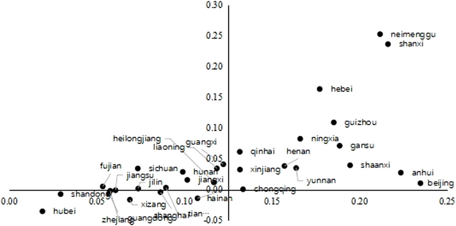
Figure 3. The Carbon Supply of Each Provinces: 2012. Notes: the horizontal axis represents the variable ${\theta }_{\overline{n}\to n}$, and the national mean is set as the origin, and the vertical axis represents the variable ${∆}_{\overline{n}\to n}$. They are all measured in percentage (%).

Figure 4

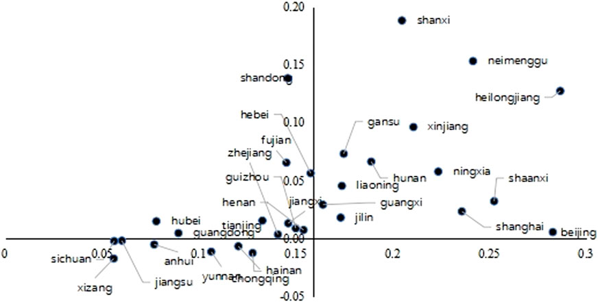
Figure 4. The Carbon Supply of Each Provinces: 2017. Notes: the horizontal axis represents the variable ${\theta }_{\overline{n}\to n}$, and the national mean is set as the origin, and the vertical axis represents the variable ${∆}_{\overline{n}\to n}$. They are all measured in percentage (%).

3.2.1 Carbon supply in each province

Figures 3, 4 depict the supply pattern for carbon content of intermediate goods in each provinces in 2012 and 2017 respectively. It is worth noting that for graphical display aesthetics, the value of ${\theta }_{\overline{n}\to n}$ and ${∆}_{\overline{n}\to n}$ in Qinghai province is too large to be shown in the graph. The unit of measurement for both the horizontal and vertical axes is percentage (%).

In the first quadrant, ${\theta }_{n\to \overline{n}}<{\overline{\theta }}_{n\to \overline{n}}\text{\hspace{0.17em}and\hspace{0.17em}}{∆}_{n\to \overline{n}}>0$. Here, $\overline{\theta }$ is the average of $\theta$. Provinces located in the first quadrant have a lower percentage of carbon supplied to other provinces compared to the national average, but the carbon emission intensity is higher than their own. So these provinces act as a domestic “pollution refuge” to some extent, even though they do not have a high supply level. In 2012, six provinces (Guangxi, Hunan, Liaoning, Jiangxi, Heilongjiang, and Sichuan) were identified as having this supply pattern of the carbon in domestic production network. The number of members adopting this pattern has increased from 6 to 10 in 2017, including Shandong, Fujian, Hebei, Jiangxi, Zhejiang, Guizhou, Henan, Tianjin, Guangdong, and Hubei, only Jiangxi remains in the first quadrant from 2012 to 2017.

In the second quadrant, ${\theta }_{n\to \overline{n}}>{\overline{\theta }}_{n\to \overline{n}}$ and ${∆}_{n\to \overline{n}}>0$. Provinces located in the second quadrant not only have a higher percentage of carbon supplied to other provinces compared to the national average, but also the carbon emission intensity of the intermediate goods supplied to other provinces is higher than their own, which can be said to be true “pollution havens” in the domestic value chain. 13 provinces adopted the supply pattern of carbon in domestic production network, namely Neimenggua, Shanxi, Guizhou, Hebei, Gansu, Shaanxi, Anhui, Beijing, Ningxia, Henan, Yunnan, Qinghai, and Xinjiang. However, the membership structure has undergone significant changes over the years. Six provinces have emerged as new entrants, namely Shanghai, Hunan, Liaoning, Guangxi, Heilongjiang, and Jilin. Six provinces have witnessed a reduction in membership, including Guizhou, Hebei, Anhui, Henan, Yunnan, and Qinghai. The final list of provinces included was Shanxi, Neimenggu, Heilongjiang, Xinjiang, Ningxia, Shaanxi, Beijing, Shanghai, Hunan, Gansu, Liaoning, Guangxi, and Jilin.

In the third quadrant, ${\theta }_{n\to \overline{n}}>{\overline{\theta }}_{n\to \overline{n}}$ and ${∆}_{n\to \overline{n}}<0$. Provinces located in the third quadrant had a higher percentage of carbon supply to other provinces than the national average. However, the carbon emission intensity of the intermediate goods supplied to other provinces is lower than their own. These provinces participate in inter-provincial carbon transfer in the domestic production network, but have not become a “pollution refuge”. This represents an optimal supply pattern of intermediate goods. Unfortunately, in both 2012 and 2017, no province was found to have the pattern of carbon supply.

In the third quadrant, ${\theta }_{n\to \overline{n}}<{\overline{\theta }}_{n\to \overline{n}}$ and ${∆}_{n\to \overline{n}}<0$. Provinces located in the fourth quadrant supply carbon to other provinces with a lower percentage than the national average, and the carbon emission intensity of the intermediate goods supplied to other provinces is also lower than their own. These provinces not only have lower degree of participation in the domestic production network, but also have lower degree of carbon supply. In 2012, there were five provinces with the pattern of carbon supply, including Hubei, Shandong, Zhejiang, Tibet, and Hainan. Although the number of members has not changed in 2017, the membership structure has changed significantly with 60.0%, Anhui, Yunnan, and Chongqing were new members, while Hubei, Shandong, and Zhejiang were no longer a member of it.

3.2.2 Evolution of the carbon supply in each province

The supply patterns of carbon in domestic production network vary among 30 provinces. These patterns are, in order from best to worst, the third quadrant III, quadrant IV, quadrant I, and quadrant Ⅱ. We can categorize the evolution of supply patterns into three scenarios: the first is the optimal (${\theta }_{n\to \overline{n}}$ ↑ and ${∆}_{n\to \overline{n}}$ ↓), the second is the sub-optimal (${\theta }_{n\to \overline{n}}$ ↓ and ${∆}_{n\to \overline{n}}$ ↓ or ${\theta }_{n\to \overline{n}}$ ↓ and ${∆}_{n\to \overline{n}}$ ↑), and the third is the worst (${\theta }_{n\to \overline{n}}$ ↑ and ${∆}_{n\to \overline{n}}$ ↑). Where the symbol “↑” indicates that the value of the variable is increasing from 2012 to 2017 and symbol “↓” indicates that the value of the variable is decreasing from 2012 to 2017. As per Table 2, from 2012 to 2017, there were six provinces in the optimal evolution state, thirteen with the worst evolution state, and eleven with the sub-optimal evolution state.

Table 2

Table 2. Changes of the carbon supply in each province from 2012 to 2017.

3.3 Net carbon supply and net value added gains and evolution of provinces in China’s production network

The net supply of carbon content of inter-provincial intermediate goods trade is denoted as $∆{\text{carbon}}_{\mathrm{n}}$, which is the total supply of carbon minus the total demand of carbon in each province and measured in millions of tonnes (MT). The added-value gains is denoted as $∆{value}_n$, which is the total added-value gains minus the total added-value expenditure in each province and measured in millions of RMB. Figures 5, 6, where the horizontal axis represents net value-added income of inter-provincial intermediate goods trade and the vertical axis represents the net supply of carbon content of inter-provincial intermediate goods trade.

Figure 5

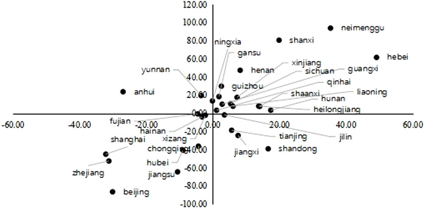
Figure 5. The Net Supply of Carbon and Value-added Gains of Each Provinces: 2012. Notes: the horizontal axis represents net value-added income and the vertical axis represents the net supply of carbon. The unit of measurement on the horizontal axis is RMB million, and the unit of measurement on the vertical axis is million tonnes (MT).

Figure 6

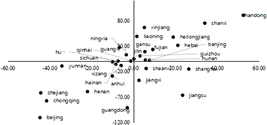
Figure 6. The Net Supply of Carbon and Value-added Gains of Each provinces: 2017. Notes: the horizontal axis represents net value-added income and the vertical axis represents the net supply of carbon. The unit of measurement on the horizontal axis is RMB million, and the unit of measurement on the vertical axis is million tonnes (MT).

3.3.1 The net carbon supply and net value-added gains

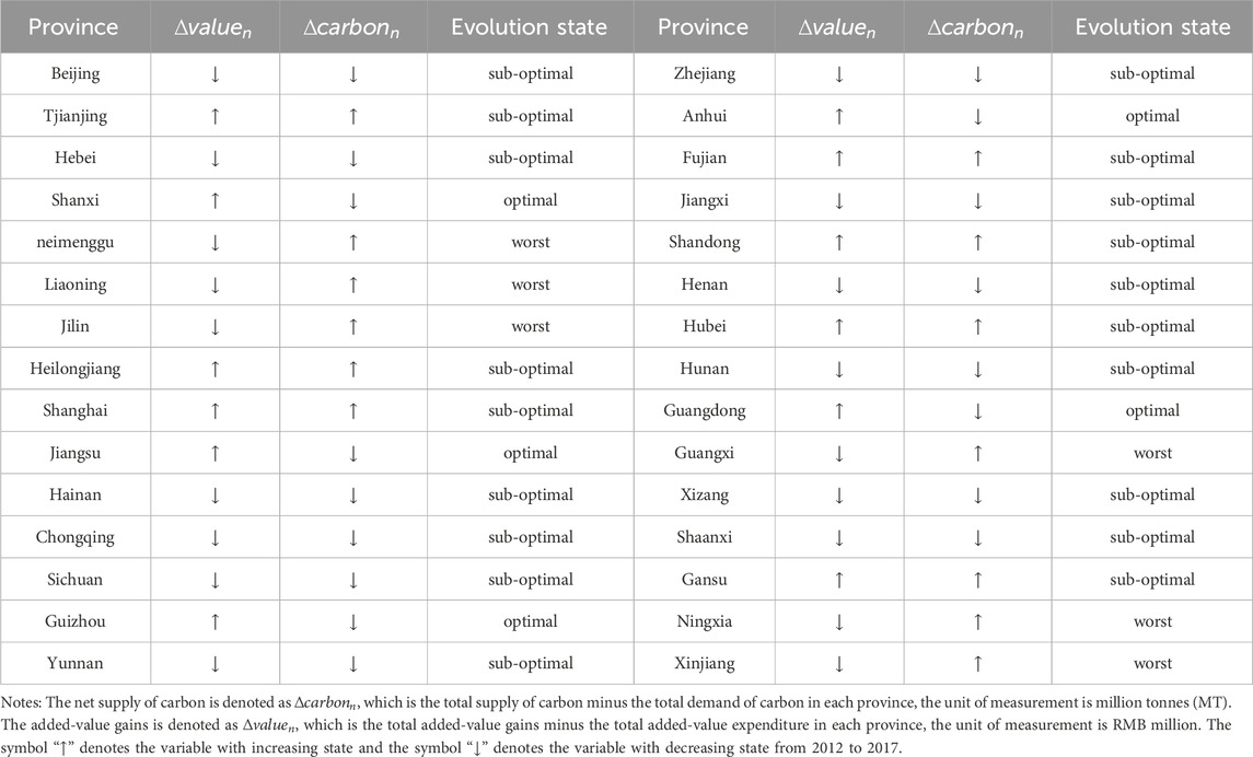
Firstly, Provinces in quadrants Ⅱ and Ⅳ of Figures 5, 6 must make a trade-off between paying environmental costs to obtain value-added income and paying value-added income to obtain environmental benefits. The provinces in the second quadrant have undoubtedly gained a net value-added benefit in domestic production network, however, that has come at significant environmental cost. On the contrary, provinces in the fourth quadrant did not experience a net value-added income, however they had significant environmental benefits. In 2012, 15 provinces are in quadrant Ⅱ of Figure 5, including Neimenggu, Hebei, Liaoning, Guangxi, Qinghai, Shanxi, Sichuan, Ningxia, Heilongjiang, Hunan, Guizhou, Gansu, Henan, Xinjiang and Shaanxi. These provinces obtain the net benefit of value-added, i.e. $∆{value}_n>0$, while also paying the environmental cost, i.e. $∆{carbon}_n>0$. In contrast, there are 9 provinces in quadrant Ⅳof Figure 5, such as Xizang, Fujian, Hainan, Chongqing, Jiangsu, Hubei, Shanghai, Zhejiang, and Beijing. These provinces pay the net economic cost, i.e. $∆{value}_n<0$, but gain the net environmental benefits, i.e. $∆{carbon}_n<0$. In 2017, the provinces located in the second and fourth quadrants of Figure 6 had the largest number of provinces as of 2012. The provinces in the second quadrant, such as Shandong, Shanxi, Xinjiang, Liaoning, Gansu, Jilin, Fujian, Heilongjiang, Hebei, and Guizhou gained net value-added income at the expense of environmental costs. The number of members has changed, with four newcomers (Shandong, Shanxi, Jilin, and Fujian) and eight dropouts (Neimenggu, Guangxi, Qinghai, Shanxi, Sichuan, Ningxia, Henan, and Shaanxi) compared to 2012. On the contrary, the provinces in the fourth quadrant of Figure 6, including Yunnan, Tibet, Hainan, Anhui, Henan, Guangdong, Beijing, Zhejiang, and Chongqing, obtained net environmental benefits at the cost of net loss of value-added income. Compared to 2012, the number of provinces increased by four and decreased by four, while the total number remained unchanged.

Secondly, there are only a few provinces that fall into quadrants Ⅰ and Ⅲ of Figures 5, 6. They represent the optimal or worst transfer patterns of carbon in domestic production network. Provinces in the first quadrant bear the net environmental costs but did not receive the corresponding net value added income, they represent the worst pattern. On the contrary, the provinces in the third quadrant not only gain net value-added income, but also experience a deficit in the carbon transfer. They represent the optimal pattern of carbon transfer. Figure 5 shows that in 2012, the provinces with the optimal pattern, including Tianjin, Jiangxi, Jilin, and Shandong, are located in the third quadrant. On the other hand, the provinces with the worst pattern, such as Yunnan and Anhui, are located in the first quadrant. Figure 6 shows that in 2017, the provinces with the optimal pattern, including Shanghai, Jiangsu, Shaanxi, and Jiangxi, are located in the third quadrant. The total number of provincial members remained the same, with Shanghai, Jiangsu, and Shaanxi being the newly added members, and Tianjin, Jilin, and Shandong being reduced compared to 2012. On the other hand, the provinces with the worst pattern, including Ningxia and Guangxi, are located in the first quadrant of Figure 6.

3.3.2 Evolution of net carbon supply and net value added gains in China’s production network

From an evolutionary perspective, a province with $∆{value}_n\uparrow \text{\hspace{0.17em}and}∆{carbon}_n\downarrow$ represents the province with the optimal evolutionary state from 2012 to 2017, a province with $∆{value}_n\downarrow \text{\hspace{0.17em}and}∆{carbon}_n\uparrow$ represents the province with the worst evolutionary state from 2012 to 2017. A province with $∆{value}_n\uparrow \text{\hspace{0.17em}and}∆{carbon}_n\uparrow \text{\hspace{0.17em}or}∆{value}_n\downarrow \text{\hspace{0.17em}and}∆{carbon}_n\downarrow$ represents the province with the sub-optimal one from 2012 to 2017. According to the report in table 3, five provinces were in the optimal evolution state, six were in the worst evolution state, and the remaining 19 were in the sub-optimal evolution state from 2012 to 2017.

Table 3

Table 3. Changes of net carbon supply and value added gains in each provinces from 2012–2017.

4 Conclusion and discussion

Due to the traditional decomposing model of the intermediate goods trade based on input-output method cannot completely account for the flow volume and its direction of intermediate goods trade, and then the carbon content of intermediate goods trade is also can not be completely accounted under the context of the domestic production network. The paper redefined the concepts of regional final output, total output, actual demand for intermediate goods, and complete demand for intermediate goods and then has constructed the calculation model of carbon content of intermediate goods trade in the domestic production network. Using China’s multi-regional input-output tables and carbon emission accounting inventory, the paper has calculated the inter-provincial circulation of carbon content of intermediate goods trade in China’s domestic production network. We have gotten some important and interesting conclusions as below:

Firstly, Between 2012 and 2017, only five provinces demonstrated a clear win-win optimization evolution between economic and environmental benefits. Conversely, six provinces exhibited a deterioration evolution, with both economic and environmental loss. Nearly two-thirds of the provinces exhibited sub-optimal evolution, with economic benefits and environmental loss, or economic loss and environmental benefits.

Secondly, the majority of provinces increase their use of high-emission intermediate goods from other provinces and lack incentives to reduce their own carbon emissions in domestic production networks. So it is becoming more and more significant to improve the mechanism of inter-provincial collaborative carbon emission reduction under the context of the domestic production network (Zhang et al., 2017; Wang, 2022). These conclusions also provide new ideas for differentiated countermeasures for water pollution management in cross-jurisdictional river basins, and for coordination of the Industrial-Ecological Economy in the Yangtze River Economic Belt, China. Specifically included: Improving the calculation model for the carbon transfer in domestic production network, and exploring the carbon emission responsibility sharing mechanism among provinces, and improving the inter-regional carbon emission compensation mechanism.

From the results of this paper’s accounting of transferring of carbon content of inter-provincial intermediate goods trade and their evolution, inter-regional environmental governance synergies have to be planned in the broader context of domestic production networks. On the one hand, those existing domestic inter-regional carbon transfer accounting models based on the entire life cycle do not involve the inter-provincial intermediate goods trade, and then can not account the inter-provincial transfer of carbon content of the intermediate goods trade. On the other hand, those inter-provincial transfer of carbon emissions accounting models based on the input-output theory, either follow the consumer principle or follow the producer principle, neglect the complete decomposition of the inter-provincial trade of intermediate goods, and thus fail to provide a theoretical basis for the accounting of the carbon content of the intermediate goods trade which includes inter-provincial inflow and outflow of a specific region at the same time. Against the backdrop of China’s growing domestic production network, the carbon content of inter-provincial intermediate goods trade is becoming an indispensable component of inter-provincial carbon responsibility accounting. The decomposition model of trade in intermediate goods developed in this paper is expected to fill the gap in this area and provide a feasible way to bridge the gap between the producer principle and the consumer principle in accounting for carbon emission responsibility.

Data availability statement

The original contributions presented in the study are included in the article/supplementary material, further inquiries can be directed to the corresponding author.

Author contributions

PY: Conceptualization, Writing–original draft, Writing–review and editing, Methodology, Software. YY: Conceptualization, Writing–original draft, Writing–review and editing, Data curation, Formal Analysis, Investigation, Resources.

Funding

The author(s) declare financial support was received for the research, authorship, and/or publication of this article. This research is supported by the National Social Science Fund of China (Grant No. 23XGJ010), and the Major Humanities and Social Sciences Research Project of Chongqing Education Commission of China [Grant NO. 22SKGH001].

Conflict of interest

The authors declare that the research was conducted in the absence of any commercial or financial relationships that could be construed as a potential conflict of interest.

Publisher’s note

All claims expressed in this article are solely those of the authors and do not necessarily represent those of their affiliated organizations, or those of the publisher, the editors and the reviewers. Any product that may be evaluated in this article, or claim that may be made by its manufacturer, is not guaranteed or endorsed by the publisher.

References

Davis, S. J., and Caldeira, K. (2010). Consumption-based accounting of CO₂ emissions. Proc. Natl. Acad. Sci. U. S. A. 107 (12), 5687–5692. doi:10.1073/pnas.0906974107

PubMed Abstract | CrossRef Full Text | Google Scholar

Du, H., Guo, J., Mao, G., Smith, A. M., Wang, X., and Wang, Y. (2011) CO₂ emissions embodied in China-us trade: input-output analysis based on the emergy/dollar ratio, Energy Policy¸ 39(10): 5980–5987. doi:10.1016/j.enpol.2011.06.060

CrossRef Full Text | Google Scholar

Du, W. J., Guan, M. X., Jiang, Y., Cao, P. H., Wang, Z., and Kang, M. Y. (2024). Whole life-cycle assessment of carbon reduction benefits of wind power in Xinjiang (in Chinese). Acta Ecol. Sin. (08), 1–10. [2024-04-02]. doi:10.20103/j.stxb.202306301400

CrossRef Full Text | Google Scholar

Gan, C., and Wang, K. (2022). Provincial spatial network structure of carbon emissions from service industry and factors in China (in Chinese). Res. Environ. Sci. 35 (10), 2264–2272. doi:10.13198/j.issn.1001-6929.2022.02.28

CrossRef Full Text | Google Scholar

Guan, Y., Shan, Y., Huang, Q., Chen, H., Wang, D., and Hubacek, K. (2021). Assessment to China's recent emission pattern shifts. Earth's Future 9. doi:10.1029/2021EF002241

CrossRef Full Text | Google Scholar

Guo-Song, M. A., and Duan, M.-S. (2024). Potential risks of double-counting carbon emission reductions in environmental rights trading and countermeasuresi(n Chinese). Clim. Change Res. 20 (01), 85–96. doi:10.12006/j.issn.1673-1719.2023.175

CrossRef Full Text | Google Scholar

Hong-ran, L. U. O., Qi-gang, ZHOU, Hui, Li, Long-jiang, W. U., Yong-fa, M. A. O., Yu-song, X. I. A., et al. (2024). Spatial correlation of land use carbon budget based on social network analysis: a case study of chongqing metropolitan area(in Chinese). Environ. Sci. 1-17. 2024-03-24]. doi:10.13227/j.hjkx.202308150

CrossRef Full Text | Google Scholar

Jie, Yu, Zhang, Y., and Qing-yao, L. I. (2024). Structural characteristics and evolutionary mechanism of spatial correlation network of carbon emissions in the Yangtze River Delta. J. Nat. Resour. 39 (02), 372–391. doi:10.31497/zrzyxb.20240209

CrossRef Full Text | Google Scholar

Ji, X., Liu, H., and Zhang, Y. (2023). Spatiotemporal evolution and driving factors of correlation network structure of China’s land-use carbon emission (in Chinese). Econ. Geogr. 43 (02), 190–200. doi:10.15957/j.cnki.jjdl.2023.02.020

CrossRef Full Text | Google Scholar

Johnson, R. C., and Noguera, G. (2012). Accounting for Intermediates,Production sharing and trade in value added. J. Int. Econ. 86 (2), 224–236. doi:10.1016/j.jinteco.2011.10.003

CrossRef Full Text | Google Scholar

Koopman, R., Wang, Z., and Wei, S. J. (2014). Tracing value-added and double counting in gross exports. Am. Econ. Rev. 104 (2), 459–494. doi:10.1257/aer.104.2.459

CrossRef Full Text | Google Scholar

Li, C., Zuo, J., Wang, Z., and Zhang, X. (2020). Production and consumption-based convergence analyses of global CO₂ emissions. J. Clean. Prod. 264 (8), 121723. doi:10.1016/j.jclepro.2020.121723

CrossRef Full Text | Google Scholar

Long, R., Li, J., Chen, H., Zhang, L., and Li, Q. (2018). Embodied carbon dioxide flow in international trade: a comparative analysis based on China and Japan. J. Environ. Manag. 209, 371–381. doi:10.1016/j.jenvman.2017.12.067

PubMed Abstract | CrossRef Full Text | Google Scholar

Los, B., Timmer, M. P., and Vries G, J. D. (2016). Tracing value-added and double counting in gross exports:comment, 106. American Economic Review, 1958–1966. doi:10.1257/aer.20140883

CrossRef Full Text | Google Scholar

Luo, X.-Yu, Cao, X.-Yu, and Song, Z.-Q. (2024). Comparison of carbon emissions throughout the entire lifecycle of buildings between China and Japan(in Chinese). Clim. Change Res. 20 (02), 220–230. doi:10.12006/j.issn.1673-1719.2023.195

CrossRef Full Text | Google Scholar

Lu, Z., and Wang, P. (2024). Study on carbon emission measurement and emission reduction effect of green buildings from the perspective of full life cycle(in Chinese). Environ. Ecol. 6 (01), 9–16+25.

Google Scholar

Muradov, K. (2016). Structure and length of value chains, SSRN working paper No. 3054155. Elsevier. Available at: https://rigvc.uibe.edu.cn/docs/2017-10/20171020085753258255.pdf.

Google Scholar

Pan, Z. (2024). Carbon emission trading activity gradually increased. Econ. Dly. 2024-2-28. (in Chinese). doi:10.28425/n.cnki.njjrb.2024.001250

CrossRef Full Text | Google Scholar

Peters, G. P. (2008). From production-based to consumption-based national emission inventories. Ecol. Econ. 65, 13–23. doi:10.1016/j.ecolecon.2007.10.014

CrossRef Full Text | Google Scholar

Peters, G. P., and Hertwich, E. G. (2008). Post-kyoto greenhouse gas inventories: production versus consumption. Clim. Change 86, 51–66. doi:10.1007/s10584-007-9280-1

CrossRef Full Text | Google Scholar

Peters, G. P., Minx, J. C., Weber, C. L., and Edenhofer, O. (2011). Growth in emission transfers via international trade from 1990 to 2008. Proc. Natl. Acad. Sci. U. S. A. 108, 8903–8908. doi:10.1073/pnas.1006388108

PubMed Abstract | CrossRef Full Text | Google Scholar

Shan, Y., Guan, D., Zheng, H., Ou, J., Li, Y., Meng, J., et al. (2018). China CO₂ emission accounts 1997-2015. Sci. Data 5, 170201. doi:10.1038/sdata.2017.201

PubMed Abstract | CrossRef Full Text | Google Scholar

Shan, Y., Huang, Q., Guan, D., and Hubacek, K. (2020). China CO₂ emission accounts 2016-2017. Sci. Data 7, 54. doi:10.1038/s41597-020-0393-y

PubMed Abstract | CrossRef Full Text | Google Scholar

Shan, Y., Liu, J., Liu, Z., Xu, X., Shao, S., Wang, P., et al. (2016). New provincial CO₂ emission inventories in China based on apparent energy consumption data and updated emission factors. Appl. Energy 184, 742–750. doi:10.1016/j.apenergy.2016.03.073

CrossRef Full Text | Google Scholar

Song, Q., Chaoqun, L. I., and Chen, J. (2024). Spatial network structure of carbon emissions and synergistic emission reduction effect in the Yangtze River delta (in Chinese). Environ. Science& Technol., 1–18. Available at: http://kns.cnki.net/kcms/detail/42.1245.X.20240315.1053.004.html.

Google Scholar

The State Council Information Office of the People's Republic of China (2021). China's Policies and Actions to address climate change. Available at: https://www.gov.cn/zhengce/2021-10/27/content_5646697.

Google Scholar

Tian, P. N., Xiao, LIANG, Guan, Y. J., YiXin, ZHAO, Mao, B. H., and Xue, T. (2024). Whole life cycle carbon emission and power generation structure transformation pathway planning of China’s power (in Chinese). Clim. Change Res. 20 (01), 97–106. doi:10.12006/j.issn.1673-1719.2023.177

CrossRef Full Text | Google Scholar

Tsagkari, M., Gaona, A., Gonzalez, J., and Jarvinen, J. (2018). The evolution of carbon dioxide emissions embodied in international trade in Poland:an input-output approach. Environ. and Socio-economic Stud. 6 (3), 36–43. doi:10.2478/environ-2018-0021

CrossRef Full Text | Google Scholar

Wang, W. (2022). Recalculation of responsibility distribution of China’s provincial consumption—side carbon emissions: based on the perspectives of shared responsibility and technical compensation (in Chinese). Stat. Res. 39 (06), 3–16. doi:10.19343/j.cnki.11-1302/c.2022.06.001

CrossRef Full Text | Google Scholar

Wang, Y., Cai, C., Zhang, D., Liu, Z., and Yiwen, L. I. (2023). Research on environmental assessment of wind power generation based on whole life cycle theory. J. North China Electr. Power Univ. Nat. Sci. Ed. 50 (06), 100–109. doi:10.3969/j.ISSN.1007-2691.2023.06.12

CrossRef Full Text | Google Scholar

Wang, Y., Wan, Lu, and Zhou, Y. (2022). Can GVC embeddings bring environmental dividends to the Belt and Road under the construction of trade channels? From the perspective of carbon embodied in trade (in Chinese). Nankai Econ. Stud. (07), 100–125. doi:10.14116/j.nkes.2022.07.006

CrossRef Full Text | Google Scholar

Wang, Z., Meng, J., Zheng, H., Shao, S., Wang, D., Mi, Z., et al. (2018). Temporal change in India’s imbalance of carbon emissions embodied in international trade. Appl. Energy 231 (1), 914–925. doi:10.1016/j.apenergy.2018.09.172

CrossRef Full Text | Google Scholar

Wang, Z., Shangjin, W., and Zhu, K. (2015). Gross trade accounting method: official trade statistics and measurement of the global value chain(in Chinese). Soc. Sci. China (09), 108-127+205–206.

Google Scholar

Weber, C. L., and Matthews, H. S. (2007). Embodied environmental emissions in U.S. International trade, 1997−2004. Int. Trade,1997-2004, Environ. Sci. and Technol. 41 (14), 4875–4881. doi:10.1021/es0629110

PubMed Abstract | CrossRef Full Text | Google Scholar

Wu, X.-fu (2019). The research review on decomposition of trade value added and global value chain status measurement (in Chinese). China Bus. Mark. 33 (04), 33–44. doi:10.14089/j.cnki.cn11-3664/f.2019.04.004

CrossRef Full Text | Google Scholar

Xu, J., Guan, Y., Oldfield, J., Guan, D., and Shan, Y. (2024). China carbon emission accounts 2020-2021. Appl. Energy 360, 122837. doi:10.1016/j.apenergy.2024.122837

CrossRef Full Text | Google Scholar

Yang, M. (2022). Research on the spatial network structure and influencing factors of carbon emissions in the yellow river (in Chinese). Inn. Mong. Univ. Sci. and Technol., doi:10.27724/d.cnki.gnmgk.2022.000122

CrossRef Full Text | Google Scholar

Yang, Q., Guo, Lu, Xing-xing, L. I. U., and Kun-qiang, ZHAO (2024). Driving characteristics of the spatial correlation pattern of carbon emissions from provincial transportation in China (in Chinese). China Environ. Sci. 44 (02), 1171–1184. doi:10.19674/j.cnki.issn1000-6923.2024.0018

CrossRef Full Text | Google Scholar

Yu, K., Feng, J., and Shi, Y. (2023). Study on the impact of China-asean regional trade on China’s carbon emission: based on GVC (in Chinese). Nankai Econ. Stud. (12), 122–143. doi:10.14116/j.nkes.2023.12.007

CrossRef Full Text | Google Scholar

Yu, Y., and Chen, F. (2017). Research on carbon emissions embodied in trade between China and South Korea. Atmos. Pollut. Res. 8 (01), 56–63. doi:10.1016/j.apr.2016.07.007

CrossRef Full Text | Google Scholar

Yue, L. V., and Yun-long, L. V. (2019). The environmental effect of China’s participation in global value chain (in Chinese). China Popul. Resour. Environ. 29 (07), 91–100.

Google Scholar

Zhang, Y., Che, Q., and Yuan, R. (2017). A research on China’s wrong disposing of essential factors and carbon emission efficiency in the perspective of supply-side reform. Academic Research. HYPERLINK. doi:10.3969/j.issn.1000-7326.2017.05.013

CrossRef Full Text | Google Scholar

Zheng, H., Bai, Y., Wei, W., Meng, J., Zhang, Z., Song, M., et al. (2021). Chinese provincial multi-regional input-output database for 2012, 2015, and 2017. Sci. Data 8, 244. doi:10.1038/s41597-021-01023-5

PubMed Abstract | CrossRef Full Text | Google Scholar