 El-Sayed M. Elkenawy
 Amel Ali Alhussan2*
 Marwa M. Eid
 Abdelhameed Ibrahim
94% of researchers rate our articles as excellent or good
Learn more about the work of our research integrity team to safeguard the quality of each article we publish.
Find out more
ORIGINAL RESEARCH article
Front. Environ. Sci. , 26 June 2024
Sec. Big Data, AI, and the Environment
Volume 12 - 2024 | https://doi.org/10.3389/fenvs.2024.1417664
Environmental issues of rainfall are basic in terms of understanding and management of ecosystems and natural resources. The rainfall patterns significantly affect soil moisture, vegetation growth and biodiversity in the ecosystems. In addition, proper classification of rainfall types helps in the evaluation of the risk of flood, drought, and other extreme weather events’ risk, which immensely affect the ecosystems and human societies. Rainfall classification can be improved by using machine learning and metaheuristic algorithms. In this work, an Adaptive Dynamic Puma Optimizer (AD-PO) algorithm combined with Guided Whale Optimization Algorithm (Guided WOA) introduces a potentially important improvement in rainfall classification approaches. These algorithms are to be combined to enable researchers to comprehend and classify rain events by their specific features, such as intensity, duration, and spatial distribution. A voting ensemble approach within the proposed (AD-PO-Guided WOA) algorithm increases its predictive performance because of the combination of predictions from several classifiers to localize the dominant rainfall class. The presented approach not only makes the classifying of rain faster and more accurate but also strengthens the robustness and trustworthiness of the classification in this regard. Comparison to other optimization algorithms validates the effectiveness of the AD-PO-Guided WOA algorithm in terms of performance metrics with an outstanding 95.99% accuracy. Furthermore, the second scenario is applied for forecasting based on the long short-term memory networks (LSTM) model optimized by the AD-PO-Guided WOA algorithm. The AD-PO-Guided WOA- LSTM algorithm produces rainfall prediction with an MSE of 0.005078. Wilcoxon rank test, descriptive statistics, and sensitivity analysis are applied to help evaluating and improving the quality and validity of the proposed algorithm. This intensive method facilitates rainfall classification and is a base for suggested measures that cut the hazards of extreme weather events on societies.
For the survival of life on earth, water is required. The social, economic, and environmental development of a region largely depends on how the region is positioned regarding water. Water accessibility influences every aspect of life, including animals, industries, agriculture, and life itself. The demand for water has gone up due to population growth, urbanization, and the need for enlarged agricultural and modernized living standards. The water cycling between the sea, atmosphere, and the earth (by rain) is a renewable resource (Raval et al., 2021). The rainfall is a major element of the hydrological cycle, and its pattern changes reflect on the water supplies. Today both hydrologists and water resource managers are worried about the changed pattern of rainfall influenced by climate change. The impact of rainfall variations is reflected in the nation’s agriculture, drinking water supply, energy industry, and many peoples’ survival. Rain is a crucial element in the management of the rise of water level of the reservoir. The reservoir could be flooded or dried because of the irregular amount of rainfall as result of climate change. Many people use rain forecasts, mostly the ones in the agriculture sector. Because the weather is always changing, forecasting rain is also very hard (Praveen et al., 2020; Samee et al., 2022).
Several factors, such as wind direction, moisture, heat, etc., that differ by region have an impact on rainfall forecasts. Therefore, a model developed for one place may not be as valuable in another (Belghit et al., 2023). The simultaneous occurrence of three patterns, namely, spatial, temporal, and non-linear, makes rainfall forecasting one of the most difficult tasks (Saha et al., 2020). Artificial intelligence algorithms can offer significant insights into a rainfall forecasting and warning system without requiring extensive knowledge of the hydrological or physical behaviors of the watershed (Barrera-Animas et al., 2022). The application of deep learning techniques for weather forecasting has grown dramatically in recent years; nevertheless, current machine learning algorithms based on observable data are only appropriate for very short-term forecasting. For medium- and short-term forecasting, numerical models are more stable, although the results may differ from the data that have been observed (Jeong and Yi, 2023).
The use of machine learning (ML) algorithms for rainfall forecasting may be advantageous. Artificial neural networks (ANN) and support vector regression (SVR) are ML techniques that are frequently used to forecast rainfall (Raval et al., 2021; Appiah-Badu et al., 2022) carried out feature engineering and chose features for each of the eight distinct classification models. They compared the efficacy of these models based on two primary criteria of F1-score and precision. A deep-learning algorithm outperformed the tested statistical models with precision of 98.26% and F1-scores of 88.61%. This demonstrated that models employing deep learning can effectively address the problem of rainfall forecasting. This work has created a variety of algorithms, various machine learning models are assessed, and their performances are contrasted to increase the precision of rainfall predictions (Hazarika and Gupta, 2020).
Accurate rainfall forecasting is a challenging procedure that requires constant progress. The proposed ensemble algorithm (AD-PO-Guided WOA Algorithm), which employs an adaptive dynamic technique, the puma optimizer (Abdollahzadeh et al., 2024), and a modified whale optimization algorithm, can predict rainfall falls under the category of conventional weather forecasting, which entails gathering and analyzing vast amounts of data. To train and test the proposed models, several optimization algorithms will be evaluated and compared for classification and model selection.
This study introduces a novel voting-based optimized algorithm for rainfall classification and forecasting, combining the Adaptive Dynamic Puma Optimizer (AD-PO) and Guided Whale Optimization Algorithm (Guided WOA). Our approach leverages multiple machine learning and metaheuristic algorithms to enhance prediction accuracy and robustness. The innovations in our approach include integrating AD-PO and Guided WOA with a voting ensemble to improve accuracy, enhancing prediction reliability through optimized parameter settings, and providing a detailed sensitivity analysis to assess model stability under various conditions.
The structure of the paper is as follows: Section 2 provides an overview of existing methods and recent advancements in rainfall forecasting and classification. Section 3 details the proposed algorithm and the datasets used in this study. Section 4 presents performance metrics and comparisons with existing models. Section 5 examines the impact of parameter settings on the model’s performance through sensitivity analysis. Finally, Section 6 summarizes the contributions of the study and suggests directions for future research.
The research interest in rainfall forecasting has recently increased because of its importance in many applications, including flood forecasting and pollutant concentration monitoring. However, most models currently used are based on complex statistical methods, which might be expensive, computationally inefficient, or difficult to apply to future tasks.
In enhancing the classification results of precipitation intensities, Belghit et al. (2023) examine the application of the AdaBoost algorithm with the One versus All strategy (OvA) and Support Vector Machine (SVM). Their study focuses on applying this model to images from the Meteosat Second Generation (MSG) satellite. The performance of the AdaBoost algorithm is compared against other multiclass SVM variants, including One Versus One SVM (OvO-SVM), Slant Binary Tree SVM (SBT-SVM), and Decision Directed Acyclic Graph SVM (DDAG-SVM). Results indicate that the AdaBoost variant, OvA-SVM, offers better performance compared to other methods. Additional classification techniques used to evaluate the model’s efficacy include Enhanced Convective Stratiform Technique (ECST), SVM, ANN, Random Forest (SART), Convective/Stratiform Rain Area Delineation Technique (CS-RADT), and Random Forest Technique (RFT). The metrics demonstrate promising results for the AdaBoost with OvA-SVM (AdaOvA-SVM) model, which significantly outperforms approaches like CS-RADT, ECST, and RFT, showcasing its efficiency in both weak and strong classifier instances, particularly in adverse environmental conditions.
Researchers are also exploring the adoption of machine learning (ML) algorithms for time series data. Barrera-Animas et al. (2022) compare simplified rainfall estimation models based on traditional machine learning algorithms and deep learning architectures. They evaluate Gradient Boosting Regressor, Support Vector Regression, Extra-trees Regressor, LSTM, Stacked-LSTM, Bidirectional-LSTM Networks, and XGBoost on their ability to forecast hourly rainfall volumes in five major UK cities using climate data from 2000 to 2020. Performance metrics include Mean Absolute Error, Root Mean Squared Error, Loss, and Root Mean Squared Logarithmic Error. The results demonstrate that Bidirectional-LSTM Networks and Stacked-LSTM Networks perform equivalently well, especially in budget-constrained applications, with low hidden layers’ LSTM-based models being the best predictors among all models tested.
Climate change and variability have worsened the ability to forecast rain accurately. However, significant progress has been made with classification algorithms to improve rain prediction accuracy. Appiah-Badu et al. (2022) evaluate the performance of different classification algorithms for rainfall prediction in various ecological zones of Ghana. The study includes Decision Tree (DT), Random Forest (RF), Multilayer Perceptron (MLP), Extreme Gradient Boosting (XGB), and K-Nearest Neighbor (KNN). Using climate data from 1980 to 2019 sourced from the Ghana Meteorological Agency, the performance of these algorithms is measured in terms of precision, recall, f1-score, accuracy, and execution time across various training and testing data ratios (70:30, 80:20, and 90:10). Results reveal that while KNN performs poorly, RF, XGB, and MLP show strong performance across all zones. Additionally, MLP consumes the most runtime resources, whereas the Decision Tree always delivers the quickest runtime.
Rainfall is crucial for water level control in reservoirs, and climatic variability poses challenges like drought or overflow. Ridwan et al. (2021) use various machine learning models and techniques to predict rainfall in Tasik Kenyir, Terengganu. Their study employs two forecasting approaches and assesses several scenarios and time horizons. Using the Thiessen polygon method to weigh station areas and projected rainfall, data is collected by averaging rainfall from ten stations around the study area. For prediction, four machine learning algorithms are used: Boosted Decision Tree Regression (BDTR), Decision Forest Regression (DFR), and Neural Network Regression (NNR). Two approaches, Method 1 (M1) involving the Autocorrelation Function (ACF) and Method 2 (M2) involving Projected Error, are evaluated. In M1, BDTR achieves the highest coefficient of determination, making it the best algorithm for ACF. Results indicate that all scenarios have coefficients within the range of 0.5–0.9, with the daily (0.9740), weekly (0.9895), 10-day (0.9894), and monthly (0.9998) forecasts having the highest values. The study concludes that while applying BDTR modeling, M1 is more accurate than M2, emphasizing the importance of considering different methods and situations in rainfall prediction.
Predicting rain and streamflow is key for wise water resource management. Ni et al. (2020) investigate the development of hybrid models for monthly rainfall and streamflow forecasts using LSTM networks, renowned for handling sequential data. The first model, wavelet-LSTM (WLSTM), uses the trous algorithm of wavelet transform for time series decomposition, enhancing the model’s ability to represent nuanced interactions and subtleties in hydrology. The second model, convolutional LSTM (CLSTM), embeds aspects of convolutional neural networks (CNNs) to capture spatial and temporal information. The accuracy of forecasts is enhanced by CLSTM’s ability to learn complex patterns and dependencies in time series data by employing the hierarchical nature of CNNs. Comparative analysis with conventional techniques like MLP and LSTM demonstrates that WLSTM and CLSTM outperform conventional methods, providing higher prediction performance and better understanding of underlying temporal dynamics. This new paradigm facilitates evidence-based decision-making and proactive action towards water-related issues in different ecological settings.
Lazri et al. (2020) aim to estimate rainfall based on pictures taken by MSG using a multi-classifier model from machine learning. For training and testing, radar and MSG satellite data correlations are noted. Six classifiers, including Weighted k-nearest Neighbors (WkNN), Random Forest (RF), ANN, SVM, Naïve Bayesian (NB), and Kmeans++, are combined for level 1 classification, where different classifiers assign a pixel to other classes. The certainty coefficients derived from these results are used as input parameters for RF in level 2 classification. This mechanism generates six classes of precipitation intensities, from extremely high to no rain. The quality of classification is significantly better with the multi-classifiers model compared to single classifiers, achieving a coefficient of correlation of 0.93. Additionally, the developed scheme shows better results than alternative methods, with biases ranging from −11 mm to 16 mm and RMSD greater than 14 mm. This approach demonstrates the potential of integrating satellite data with machine learning models to enhance rainfall forecasting accuracy.
Avanzato et al. (2020) addressed the increasing occurrence of natural disasters due to hydrogeological instability caused by heavy rain. To mitigate these risks, the study emphasized the need for accurate precipitation estimation using advanced machine learning techniques. The researchers introduced the AVDB-4RC (Audio/Video Database for Rainfall Classification) dataset, which includes audio and video data recorded by a custom-built multimodal rain gauge. This dataset categorizes rainfall into seven intensities: “No rain,” “Weak rain,” “Moderate rain,” “Heavy rain,” “Very heavy rain,” “Shower rain,” and “Cloudburst rain.” The validation of the dataset involved a novel rainfall classification method using Convolutional Neural Networks (CNNs), achieving an average accuracy of 49%, which could improve to 75% when excluding adjacent misclassifications. This study is notable for providing the first open dataset combining acoustic and video data for rainfall classification, encouraging the evaluation and improvement of rainfall estimation algorithms on a shared platform.
Table 1 provides a concise overview of the methodologies, performance metrics, and key findings of each study.
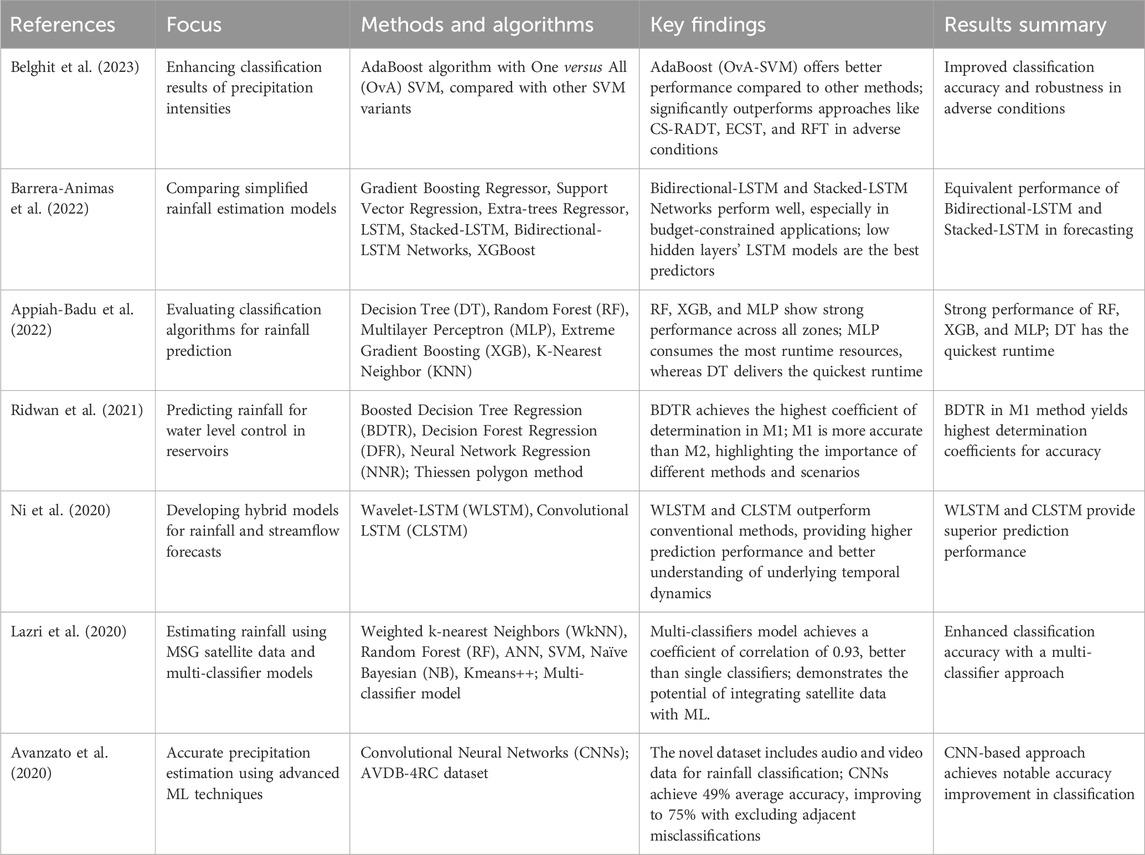
Table 1. Rainfall classification and forecasting related works summary.
This section delves into the AD-PO-Guided WOA algorithm as shown in Figure 1, which employs an adaptive dynamic technique, the puma optimizer, and a modified whale optimization algorithm. Algorithm 1 provides a depiction of the AD-PO-Guided WOA algorithm.
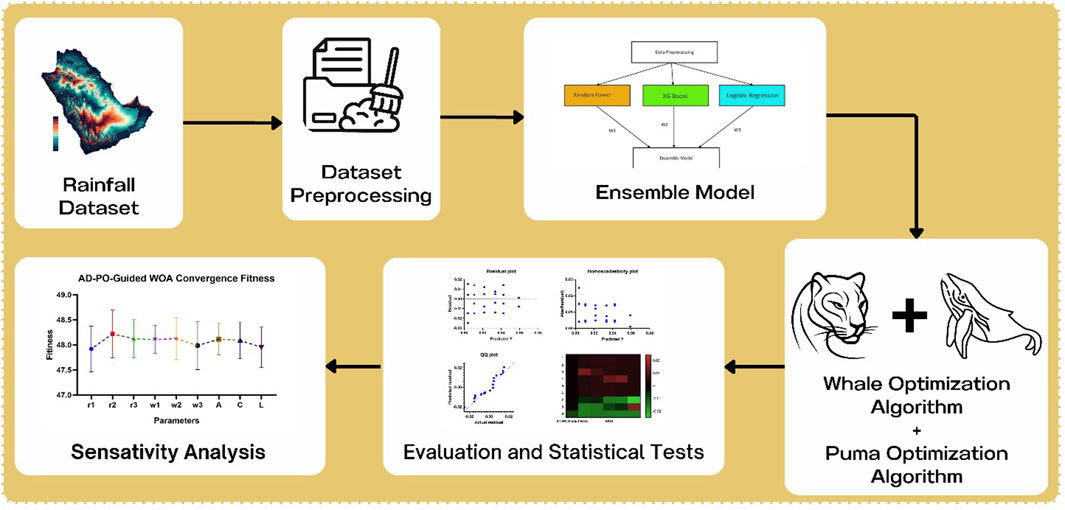
Figure 1. The proposed framework for AD-PO-guided WOA algorithm.
Following the initialization of the optimization algorithm, a fitness value is assessed for each solution within the population. The algorithm identifies the solution with the best fitness value as the best agent. Initiating the adaptive dynamic process involves segregating the population into two distinct groups. These groups are referred to as the exploitation group and the exploration group. The primary objective of individuals in the exploitation group is to converge toward the optimal or best solution, while individuals in the exploration group aim to explore the vicinity around the leaders. The update process among the population groups’ agents operates dynamically. To maintain a balance between the exploitation group and the exploration group, the optimization algorithm commences with an initial population distribution of (50/50).
The WOA algorithm demonstrates its efficacy across various optimization problems. It is widely acknowledged in the literature as one of the most powerful optimization algorithms (El-Kenawy et al., 2020). However, a potential drawback lies in its limited exploration capabilities (Mirjalili et al., 2020; Ghoneim et al., 2021). For mathematical purposes, let’s denote ‘
In Eq. (1), the term
In Eq. (2), the three random solutions are denoted as
where,
The Puma Optimizer (PO) (Abdollahzadeh et al., 2024) is a bio-inspired metaheuristic algorithm that has been created to solve optimization problems with efficiency and adaptability. Developed based on the hunting activities of pumas, the PO algorithm applies a multi-stage strategy, which includes the stages of exploration and exploitation. As shown in Figure 2 In the exploration phase, like a puma, as it tours the territory in search of possible prey, the algorithm does the random exploration of the search space in order to find new solutions. While doing so, it also avoids the local optima. In the exploitation phase, on the contrary, the algorithm emulates pumas’ hunting methods—ambushes and sprints-to improve existing solutions and exploit promising areas of the search space. Using heuristic selection algorithms and hyper-heuristic mechanisms, the PO adaptively changes its strategies based on the problem landscape and historical information to optimally balance between exploration and exploitation to converge to optimal solutions quickly.
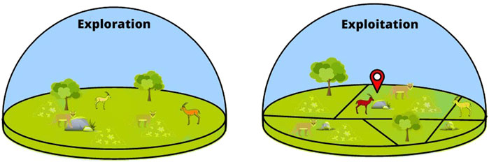
Figure 2. PO exploration and exploitation process.
Utilizing nature-inspired insights and adaptive strategies from pumas, the Puma Optimizer provides an efficient and flexible solution for optimization problems. The design of the method is multi-phase and enables the comprehensive investigation of different solution spaces and the focused extraction of attractive regions, which results in high-quality solutions being found. Due to its flexible nature and effectiveness, the PO algorithm has a powerful ability to address many optimization problems in different domains and is also, therefore, a critical tool in the sphere of computational optimization. Algorithm 1 shows the pseudo-code of the puma optimizer.
Algorithm 1.Pseudo-code of PO.
% PO setting
Inputs: The population size N and the maximum number of iterations and parameter settings
Outputs: Puma’s location and fitness potential
% initialization
Create a random population using Xi (i = 1, 2, …, N). Calculate Puma’s fitness levels.
For iter = 1: 3
Apply exploration phase
Apply exploitation phase
End
Apply Unexperienced Phase
for iter = 4: Max iteration
Apply experienced Phase
if Score Explore > Score Exploit
Apply exploration phase (Algorithm 1)
if Exploration NewBestXi Cost < Puma male Cost
Puma male = NewBestXi
end
else
Apply exploitation phase (Algorithm 2)
if Exploitation NewBestXi Cost < Puma male Cost
Puma male = NewBestXi
end
end
Update
Update Score Explore and Score Exploit by Eq. 17
end
This section provides a complexity analysis of the AD-PO-Guided WOA algorithm using Algorithm 1. By denoting the population number as
• Initializing the population
• Initialize the set of parameters
• Assess the fitness function
• Gaining the best individuals
• Update the position
• Assessing the fitness function of agents through the utilization of Guided WOA
• Assessing the fitness function of agents through the utilization of PO
• Update
• Best solution updating
• Increasing the counter iteration
The computational complexity of the AD-PO-Guided WOA algorithm can be expressed as
The effectiveness of an optimizer is gauged by evaluating the fitness function (Hassan et al., 2022), primarily reliant on the classification/regression error rate and the selected features from the input dataset. The optimal solution is determined by a set of features that minimize both the feature count and classification error rate as shown in Eq. 4. The assessment of solution quality in this study is carried out using the following equation.
where the error rate of the optimizer is denoted as
The voting classifier model is based on Adaptive Dynamic Puma Optimizer (AD-PO) and augmented with the Guided Whale Optimization Algorithm (Guided WOA) as outlined in Algorithm 2. The AD-PO-Guided WOA algorithm combines RF and XG Boost classifiers to enhance the accuracy of the ensemble. The classifiers undergo training to determine optimal weights. The AD-PO-Guided WOA algorithm is then employed to optimize these weights.
Algorithm 2.AD-PO-Guided WOA Algorithm.
Set the population
Set the parameters
Assess the fitness function
Identify the most optimal individual
while
if
for
if
if
Update the position of current search agent as
else
Select the search agents
Update
Update the position of current agent as
end if
else
Update the position of current agent as
end if
end for
Calculate the fitness function
else
Calculate the fitness function
end if
Update
Find the best individual
Set
end while
return
A Random Forest (RF) is a type of ensemble learning method that merges the predictions from numerous decision tree, aiming to enhance overall performance and resilience (Zaki et al., 2023). Random forest is constructed upon the fundamental principles of decision tree, which are basic models systematically dividing the data based on features for prediction purposes. Instead of employing all features for every split within each tree, the random forest algorithm opts to randomly choose a subset of features for each decision tree (Rodriguez-Galiano et al., 2012). This variability contributes to the creation of diverse trees. Every tree is constructed using a random sample, drawn with replacement, from the original dataset. This technique is commonly referred to as bootstrapped sampling. When dealing with a new data point, each decision tree within the forest provides a prediction for the class. The ultimate prediction is determined by the class that attains most votes across all trees (Parmar et al., 2019). The quantity of decision tree within the forest is a vital hyperparameter. Elevated numbers generally result in improved performance, reaching a stage of diminishing returns. The maximum depth hyperparameter determines the complexity of individual trees.
Extreme Gradient Boosting, commonly referred to as XG Boost stands out as a potent and effective machine learning algorithm celebrated for its exceptional performance across diverse data science applications. XG Boost falls under the ensemble learning umbrella, specifically leveraging boosting techniques (Chen et al., 2015). It amalgamates predictions from multiple weak learners, typically decision tree, to construct a resilient model. XG Boost introduces a regularization term in the objective function. This addition enhances the model’s capability to manage complexity and counteract overfitting. XG Boost sequentially builds a series of decision tree, each rectifying errors from its predecessor (Osman et al., 2021). To control individual tree complexity and prevent overfitting, the algorithm integrates L1 (LASSO) and L2 (ridge) regularization terms. The algorithm optimizes an objective function that combines a loss function, gauging model performance, and a regularization term during the training process.
The K-Nearest Neighbor (KNN) classification algorithm is a straightforward yet impactful supervised machine learning method applicable to both classification and regression tasks (Rizk et al., 2023). KNN operates based on the premise that similar instances or data points typically reside closely together in the feature space. For classification purposes, when presented with a new, unlabeled data point, KNN determines its class by examining the majority class among its K nearest neighbors. The algorithm relies on a distance metric, often Euclidean distance, to gauge the proximity between data points (Suguna and Thanushkodi, 2010). Alternative metrics like Manhattan distance can be employed depending on the specific problem. ‘K' signifies the number of nearest neighbors to consider. This pivotal hyperparameter significantly influences the model’s performance. A smaller ‘K' may yield a more responsive model, while a larger ‘K' introduces more smoothing. KNN does not explicitly construct a model with a defined decision boundary. Instead, it classifies new data points based on the consensus of their K nearest neighbors.
The Decision Tree (DT) classification algorithm stands out as a versatile and extensively utilized supervised machine learning approach, catering to both classification and regression tasks (Priyam et al., 2013). DT adopts a hierarchical structure resembling a tree. Each internal node serves as a decision point based on a feature, branches represent outcomes, and leaf nodes denote the final class or predicted value. At each decision node, the algorithm assesses a feature and makes decisions using criteria like Gini impurity or information gain. This process iterates until a specified stopping condition is met. The choice of criteria for splitting nodes is pivotal, with common measures including Gini impurity for classification tasks and mean squared error for regression tasks. The objective is to maximize homogeneity within nodes (Patel and Prajapati, 2018). DT provides a metric for feature importance, highlighting features that significantly reduce impurity or variance as more influential in decision-making. To address overfitting and the capture of noise in training data, DT undergoes pruning, involving the removal of branches that contribute little predictive power, fostering a more generalized model (Li and Belford, 2002). A key strength of DT lies in its interpretability. The resulting tree structure offers a clear understanding of the decision-making process. DT exhibits flexibility in handling both categorical and numerical data, employing distinct splitting strategies for each data type.
These methodologies aim to leverage the unique strengths of various individual base models in building a predictive model. This concept can be implemented through diverse means, with notable strategies encompassing the resampling of the training set, the exploration of alternative prediction methods, or the adjustment of parameters in specific predictive techniques. In the end, the results from each prediction are combined through an ensemble of approaches.
Forecasting models are extremely important in the prognosis of future trends and patterns from historical data. Here, we discuss four commonly used forecasting models including Baseline, autoregressive integrated moving averages (ARIMA), seasonal ARIMA (SARIMA), and long short-term memory (LSTM) networks. The Baseline model acts as a basic reference to compare with more advanced forecasting approaches. It usually implies the prediction of future values through the mean or median interpolation of historical data. Although too primitive, the Baseline model is used to measure the power of more sophisticated models and can occasionally give surprisingly accurate predictions to stable time series data. ARIMA is a widely used time series forecasting model appreciated for its flexibility and ability to capture temporal dependencies. ARIMA models are characterized by three components: First order autoregression (AR (1)), differencing (I (1)), and first-order moving average (MA (1)). The autocorrelation, as well as the partial autocorrelation functions of the time series data, when analyzed by ARIMA models, can help identify and model the underlying patterns and seasonality, which makes ARIMA models suitable for a variety of time series forecasting (Hazarika and Gupta, 2020).
SARIMA (Seasonal ARIMA) adds an ability to ARIMA models to consider seasonal attributes in the forecasting process. SARIMA models are especially recommended for time series data that has seasonal patterns or trends, such as monthly and quarterly data. Seasonal differencing and seasonal autoregressive and moving average terms included in SARIMA models enable them to adequately reflect seasonal fluctuations present in the data and, therefore, enhance the accuracy of forecasting. LSTM networks are a type of RNNs that are later developed to model long-term dependencies in sequential data. LSTM models are good at capturing difficult temporal patterns and nonlinear relationships in time series data, which makes them especially suitable for time series forecasting tasks. Utilizing a chain of connected memory cells, LSTM models can essentially learn and store patterns across longer time spans, thus providing precise forecasts despite the presence of noisy or erratic data. Each forecasting model has its unique advantages and features that make it feasible for different forecasting problems and data types. It is important to know the characteristics and limitations of each model to choose the best approach for a certain forecasting situation.
In this section, the materials and methods employed in two distinct scenarios of manipulation and tendencies are outlined. In a classification scenario, the technique that is used to classify data or groups defined by a set of criteria is explained. This is the step where you will be concerned with the selection of data mining algorithms, feature engineering techniques and performance evaluation metrics. Moreover, in the scenario of forecasting, a list of forecasting models will be applied, in addition to data preprocessing and metrics to check forecast accuracy. The aim is to give particulars about the materials and methods simultaneously for the group’s classification and forecasting by providing the full description of the research methodology applied in this study.
The dataset used in this paper is available at (Classification Scenario, 2024). This dataset encompasses the cumulative precipitation (in millimeters) recorded by PME MET (Presidency of Meteorology and Environment) stations in Saudi Arabia, provided by the General Authority for Statistics. The data spans from 2009 to 2019 for up-to-date information relevant to advancing research in energy economics. The dataset attributes include region, which indicates the region in Saudi Arabia where the meteorological station is located; station, which specifies the meteorological station within the region; total rainfall, which is observed in millimeters for each month of the year, rainfall intensity: that is a quantitative measure of the amount of rainfall, usually in millimeters or inches. This could be provided as a single value or broken down into intervals (light, moderate, heavy, etc.); duration is the length of time over which rainfall occurs, expressed in minutes, hours, or days. Rainfall type: is the classification of rainfall into categories, such as rainy or not rainy, and rainfall distribution represents the information about how rainfall is distributed over a specific period, including whether it is continuous or intermittent.
The dataset includes detailed attributes relevant for classification purposes:
• Total Rainfall (mm): Observed in millimeters for each month of the year, indicating the cumulative precipitation recorded by each station.
• Wind Speed: The average wind speed recorded during the observation period, which can influence rainfall patterns.
• Humidity: The average humidity level recorded, which is a critical factor in precipitation formation.
• RainTomorrow: A binary indicator (Yes/No) signifying whether it rained the next day, used for predicting future rainfall events.
• Month: The specific month of the year when the data was recorded, helping to identify seasonal patterns.
Data preprocessing plays a pivotal role in the machine learning and metaheuristic process, encompassing activities like cleaning, transforming, and integrating data to prepare it for analysis (Khafaga Doaa et al., 2022). The primary objective of data preprocessing is to enhance the quality of the data and tailor it to meet the requirements of the data mining task at hand. Data preprocessing, integral to the data preparation phase, encompasses various processing activities applied to raw data to ready it for subsequent processing steps (Alkhammash et al., 2022). Historically, it has served as a crucial initial stage in the data mining process. In more contemporary contexts, the methods of data preprocessing have evolved to cater to the training of machine learning, Artificial Intelligence (AI) and metaheuristic algorithms, as well as for executing inferences based on them. Real-world data is frequently disorderly, generated, processed, and stored by diverse individuals, business procedures, and applications (Tarek et al., 2023). Consequently, a dataset might lack specific fields, exhibit manual input inaccuracies, or include duplicate data, as well as variations in names denoting the same entity (Khafaga D. et al., 2022). While humans can typically recognize and address these issues in the data used for business operations, data employed to train machine learning, deep learning and metaheuristic algorithms necessitates automated preprocessing (Alkhammash et al., 2023).
The role played by the total rainfall and accompanied humidity in Weather phenomena and patterns of precipitation is undeniable. Figure 3 shows the Correlation heat map of the original dataset to visualize the patterns between different variables. This is shown in the figure below. Correlation heatmaps are a means of visualizing the degree and sign of linear relationship between pairs of variables, whereby warmer colors indicate stronger positive correlations and cooler colors stand for stronger negative correlations. This representation helps in finding the trends and connections in the data. In addition, it makes the feature selection process easy and provides opportunities for exploring the data aspects more deeply. Understanding the associations of various meteorological parameters and applying them to predict rainfall better helps researchers include the most significant variables and formulate classification models of higher efficiency and precision.
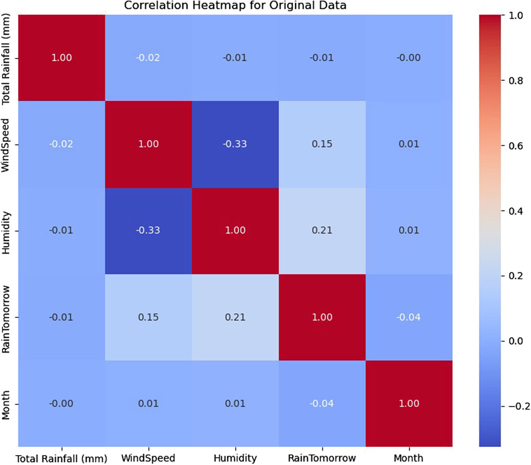
Figure 3. Correlation heatmap for original data.
Copula analysis is a statistical method used to model the dependence structure between multiple random variables. Unlike traditional correlation measures, which only capture linear relationships, copulas allow for the characterization of complex dependencies, including non-linear and tail dependencies (Benali et al., 2021). Figure 4 illustrates a 3D scatterplot correlation between humidity and the copula dataset. Copulas represent a class of statistical techniques to model the interdependencies among many variables; hence, this picture is essential for understanding the complicated associations with humidity as well as other climate factors. Researchers can then exploit this in-depth knowledge of the dynamics of humidity of this data set. The visualization concerned helps the investigators in revealing the order and behavior of the variables, which are hard to detect when only the separate individual variables are being analyzed. The wind speed could be plotted along one axis, whereas the two additional variables could be plotted along the other axes (Bahraoui et al., 2018; Petropoulos et al., 2022). Such a scatterplot gives a good snapshot of how wind speed interrelates with their other atmospheric factors.

Figure 4. 3D scatterplot of humidity in copula data.
To analyze the Climatic Research Unit (CRU) data, we utilized the CRU TS interface integrated into Google Earth. This integration facilitates renewable energy investment by creating a diversified and resilient electricity grid. The user interface (UI) provides an intuitive way to specify study areas and load the required climate data. Datasets are updated annually, and for this study, we used data spanning from 1901 to 2020, offering a century-long perspective to enrich our research.
The CRU TS site (Harris et al., 2014; CRU, 2024) is straightforward to navigate, allowing easy access to climate data. Specifically, for our analysis, we extracted data on average monthly rainfall in Mecca, Saudi Arabia, using the Google Earth Pro platform. This dataset was instrumental in training our algorithm, enabling us to develop highly efficient models for rainfall analysis and prediction.
Combining the strengths of Google Earth Pro with the CRU TS interface allowed us to explore global climate data and tailor our analysis to local conditions in Mecca. This approach ensured that our models were not only accurate but also highly relevant to the specific climatic patterns of the region.
Our analysis will be preceded by the preprocessing of the climate data that we have retrieved from the CRU TS interface within Google Earth Pro. The preprocessed data will undergo careful, meticulous processing. The most crucial task at this point is to undertake a form of tuning of the data so it can be properly processed, entailing a high degree of accuracy. First, we completed a thorough scrubbing procedure by fixing and squaring any inconsistencies, errors, or missing data. This first step was surely the most important one in terms of ensuring the correctness and reliability of the dataset, which is paramount for our following analysis. Thereby, a solid basis for our upcoming efforts will be created. Upon completing cleaning, the normalization technique was used to standardize the range of values of different variables so that they could be subjected to a fair comparison with no scale variations. In the next step, we chose the top features based on the scores of our features selection process to validate the most important variables. This helped us focus our data analysis and reduce the computation complexity without losing important data. Additionally, spatial and time aggregation methods were used to compress the dataset, making it more manageable and still capturing the complex components, broader meaning, and patterns. Another aspect that we did was careful outlier detection and removal to increase the dependability of our findings and make the model more sensible to deviations. While applying elaborate and careful data preprocessing that involves data cleaning, normalization, feature selection, spatial and temporal aggregation, and outlier detection, we achieved data/raw data refinement at the needed level on a quality, reliability, and suitability basis for subsequent analytical steps.
Figure 5 presents a detailed visualization of the CRU data, showcasing three key components: the residual, seasonality, and trend. The plot represents a term interpretation of the time series embedded in the data, bringing to light many important facts, such as trends and patterns that happen over time. The residual quantity aimed at insinuating a component of variation in the data that cannot be due to seasonal and trend-related causes is critical in the process of conditioning and identification of outliers and irregularities. Also, the seasonality component reveals reoccurring patterns or fluctuations that happen periodically (i.e., annually or monthly). Therefore, there is an ability to perceive clear trends such as annual temperature fluctuation or monthly rainfall patterns. The last part, which is the trend component, portrays the long-run trajectory or directionality of the data and therefore, one can easily identify the trend, such as temperature increase or slope decline. In other words, the whole battery of basic information provided by the CRU data allows researchers to detect hidden patterns, trends, etc. and improve their knowledge about climate variability and change.
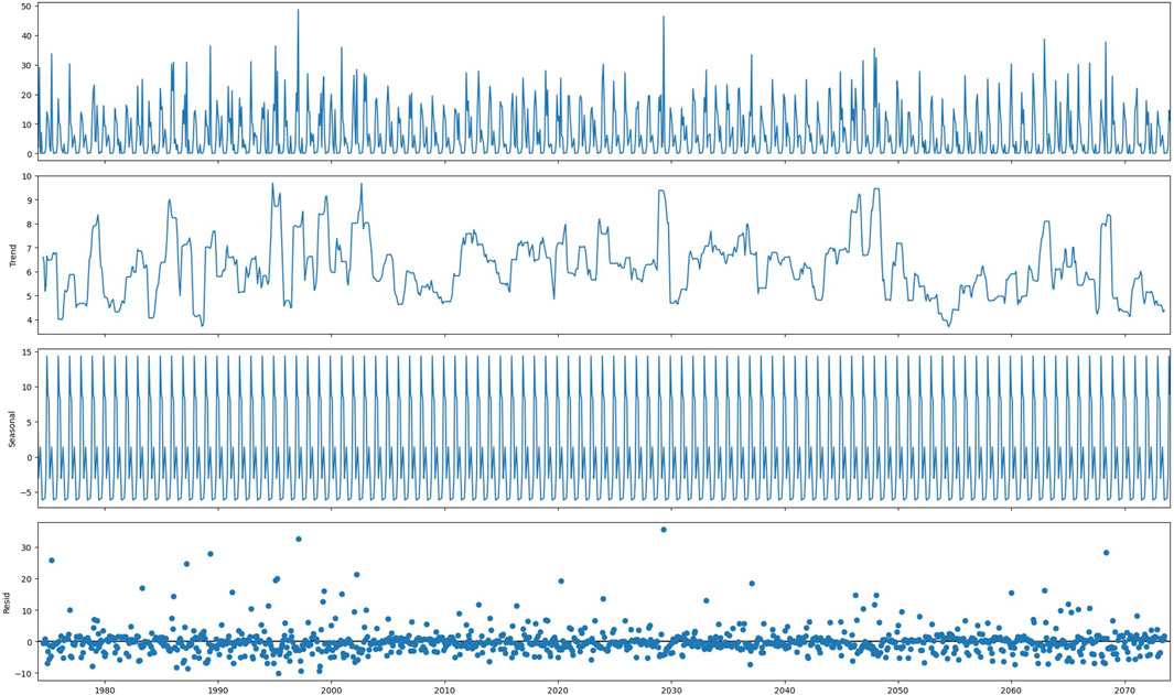
Figure 5. Residual, seasonality, and trend plot for the CRU data.
This section presents the experimental results obtained which is divided into two main categories based on classification-scenario outcomes and forecasting-scenario outcomes. In the classification scenario, different algorithms are evaluated in their ability to classify data into predefined classes. In the forecasting scenario, however, the performance of forecasting models is analyzed as to their capacity of prediction based on history of the tested data. A comprehensive analysis of the results from both scenarios provides crucial information on the effectiveness of the methodologies proposed in this work and their impact on real-life situations. By conducting an in-depth analysis of the experimental results, this research aims to find some useful implications about the strengths and limitations of the classification algorithms and forecasting models, which would help move forward the data-driven analysis and prediction.
In the classification scenario, several machine learning algorithms were assessed for their effectiveness in categorizing data into pre-assigned classes using defined criteria. The experiments were carried out with different classification methods. Detailed results of these experiments, which include metrics like accuracy, precision, recall, and F1-score, were presented and discussed. Also, the strengths and weaknesses of each classification algorithm were described, and any interesting findings or matters learned from the experiments were outlined.
The aim idea is to assess the effectiveness of the suggested voting optimizer, specifically the AD-PO-Guided WOA algorithm, in enhancing the classification accuracy of rainfall. To substantiate the superiority of the proposed algorithms statistically, Wilcoxon’s rank-sum test and descriptive statistics are conducted. The dataset is randomly divided into training (80%), and testing (20%) sets for experimentation. The initial experiment displays the outcomes for RF, XGBoost, KNN, and DT employed as individual classifiers, as outlined in Table 2. The classifier performances are delineated across data preprocessing. Table 2 highlights that the RF, and XG Boost classifiers achieved the highest accuracy, sensitivity, specificity, PPV, NPV, and F-score. The outcomes for comparing the proposed voting algorithm against other voting algorithms utilizing PSO, AD-PO-Guided WOA, WOA, Grey Wolf Optimization (GWO), and Genetic Algorithm (GA) are presented in Table 3. The results indicate that the AD-PO-Guided WOA algorithm, with an accuracy of 0.95993, surpasses the performance of PSO (accuracy = 0.94,642), voting Guided WOA (accuracy = 0.93829), voting WOA (accuracy = 0.92637), GWO (accuracy = 0.91476), and GA (accuracy = 0.90,793). The AD-PO-Guided WOA algorithm gives competitive results with sensitivity of (0.9842519), specificity of (0.86956521), PPV of (0.92592592), NPV of (0.970873786), and F-score of (0.954198) compared to other voting algorithms.
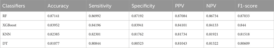
Table 2. Performance of the outcomes from single classifiers.
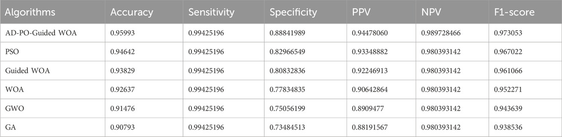
Table 3. Comparing the proposed algorithm with other voting algorithms.
Table 4 provides a comprehensive overview of the descriptive statistics for the showcased optimizing ensemble algorithm in comparison to alternative algorithms. The analysis using Wilcoxon’s rank-sum test (Breidablik et al., 2020; Khadartsev et al., 2021), as outlined in Table 5, aims to discern any noteworthy differences in the results among the models. A p-value below 0.05 signifies substantial superiority. The findings not only highlight the superior performance of the AD-PO-Guided WOA algorithm but also emphasize the statistical significance of the algorithm itself.
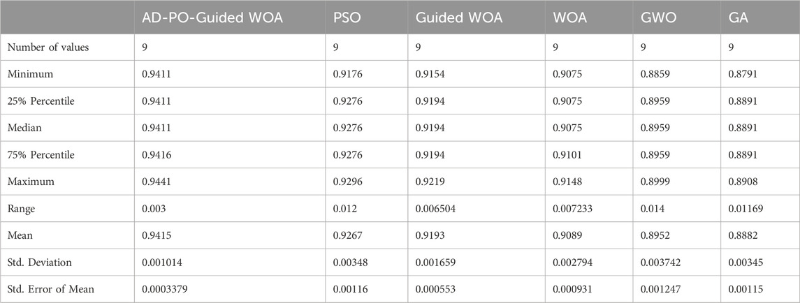
Table 4. The proposed algorithm descriptive analysis versus another voting algorithms.
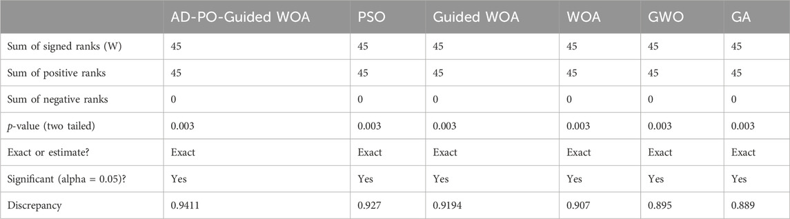
Table 5. The Wilcoxon signed rank test findings for the proposed algorithm in contrast to alternative algorithms for rainfall classification.
Figure 6 illustrates the AD-PO-Guided WOA algorithm, based on the objective function, in comparison with various other algorithms.
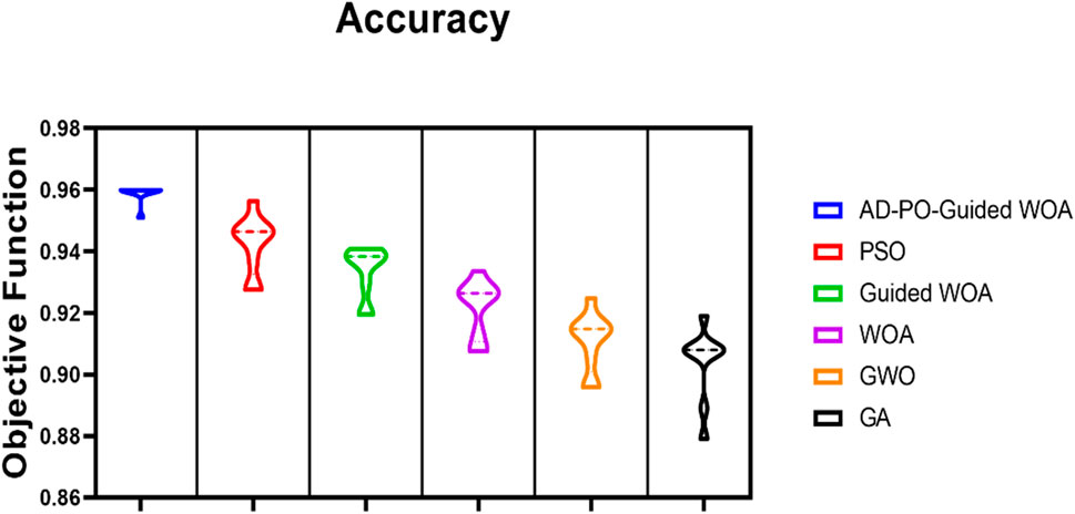
Figure 6. The AD-PO-Guided WOA algorithm accuracy is based on the objective function compared to different algorithms.
In the forecasting scenario, predictive accuracy was checked about various forecasting models in the prediction of future trends or outcomes from utilized historical data. The experiments were performed using different forecasting methods, including ARIMA, seasonal ARIMA (SARIMA), and LSTM networks. The findings of these experiments, which include mean absolute error, root mean squared error, and other related measures, were further elaborated and discussed. In addition, the performance of each of the forecasting models was compared, and the factors influencing their predictive accuracy were examined.
The results of the comparison of the forecast models are presented in Table 6, in which baseline, ARIMA, SARIMA, LSTM, and AD-PO-Guided WOA-LSTM are included. The table contains some performance measures such as MSE, RMSE, MAE, MBE, r,
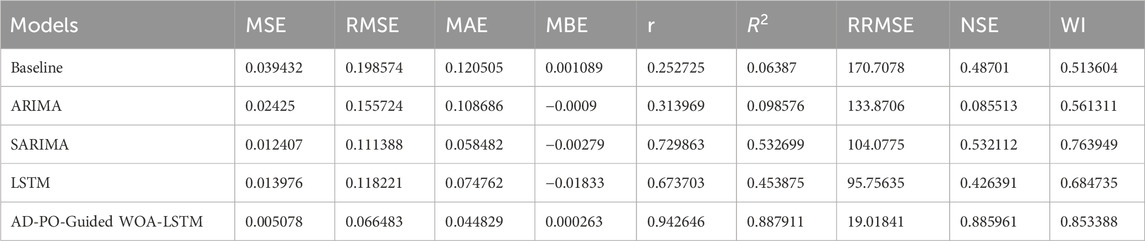
Table 6. Compression of forecasting results.
Figure 7 demonstrates the residual plot of the model and, hence, hints at the deviations between expected and observed values. Residuals are an index to measure the difference between the true values and the values predicted by the model. The residual plot is a powerful tool for the model assessment that shows if data contain any regression pattern, which indicates its predictive power. In the case of an ideal scenario, the residuals should be just scattered around zero, and that proves that the model does not have any bias and its prediction is compelling and precise. However, the residuals’ memory may suggest that our model might be lacking some important features or may not include all the features of the data. By these test plots, model makers can know how good the model is and where the smoothing is done in order to improve.
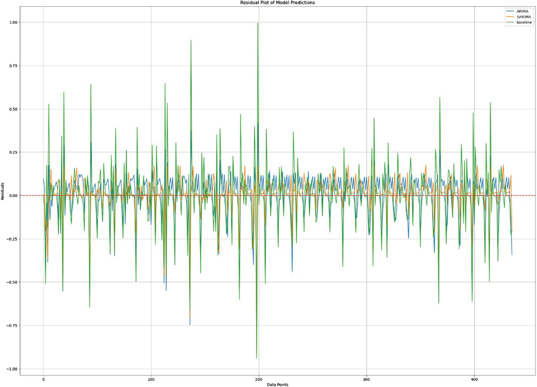
Figure 7. Residual plot of model predictions.
Figure 8 displays the forecasting and genuine rainfall in Mecca to get a real picture of the forecasting and the measurement values. This plot demonstrates the model’s performance in terms of precision and reliability in generating forecasts of rainfall patterns in the coming years. Points or markers usually represent the historical data, and lines or curves represent the forecasts.
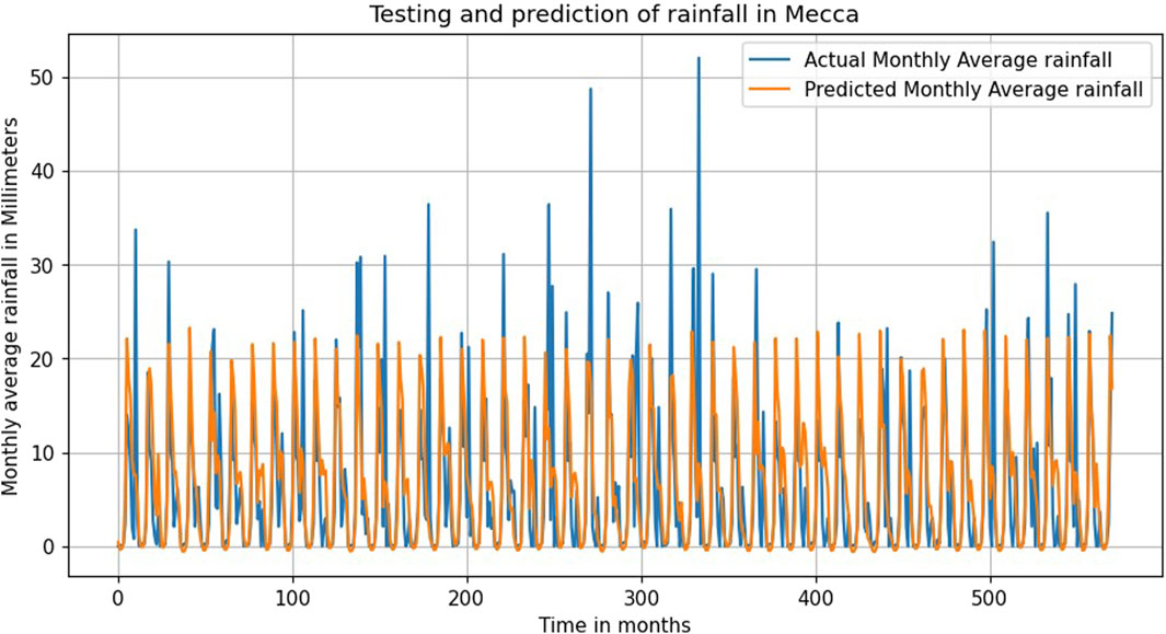
Figure 8. Testing and prediction of rainfall in mecca.
Figure 9 represents the simulation and forecasting of LSTM rainfall in Mecca through the graphical explanations of the model, as the performance is delivered by the Long Short-Term Memory (LSTM) model on predicting the trends of rainfall. This kind of graphic is mostly preferred to display the Rainfall values for both observed and LSTM model forecast predictions so that a direct comparison between the two can be easily made. Obtained values become data points or markers, whereas the predicted values, which are more likely to be represented as a line or curve, are shown as a continuous line or curve.
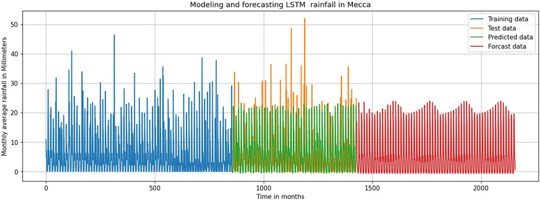
Figure 9. Modeling and forecasting LSTM rainfall in Mecca.
Figure 10 represents a heatmap comparing the AD-PO-Guided WOA-LSTM model with others and gives visual insights into their performances varying by different metrics. The heatmap is an effective tool to track performance patterns and trends as the color gradient is used to ascertain varying levels of model performance across all the measures. Figure 11 displays a parallel plot representing how the AD-PO-Guided WOA-LSTM model beats the other models. A peculiarity of this plot is the ability to conduct a detailed comparative study of several models simultaneously with respect to several performance criteria concurrently. Every line represents a different type of model, and the plots on the axes represent their performance on each metric, therefore enabling us to make quick comparisons and spot the areas of strength and weakness. Figure 12 depicts a radar plot that shows the performance metrics of the AD-PO Guided WOA-LSTM model alongside the other models.
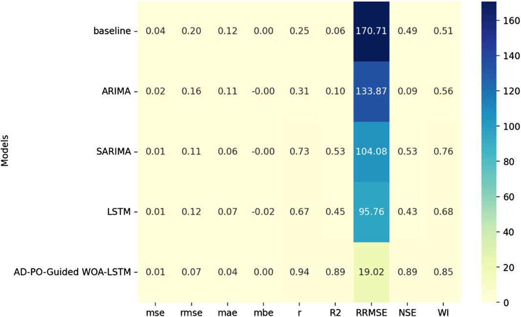
Figure 10. Heatmap Compression of AD-PO-Guided WOA-LSTM and other Models.
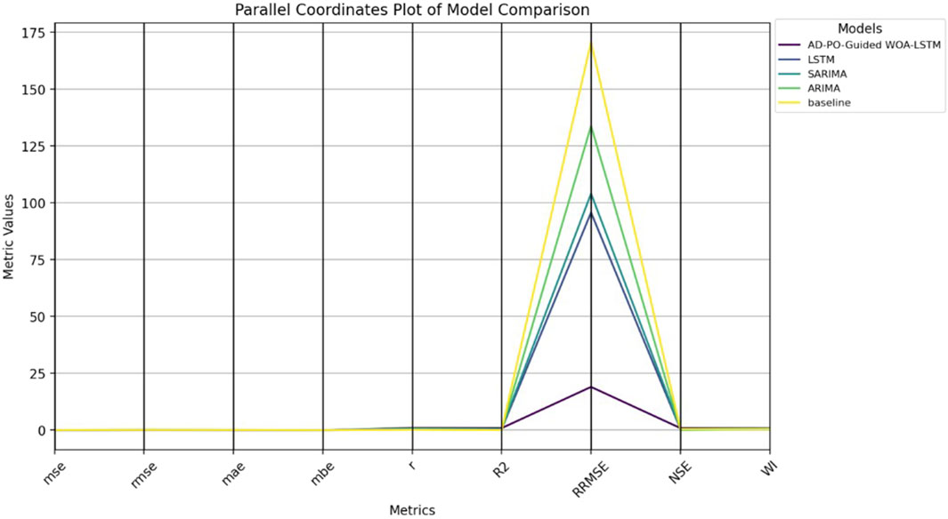
Figure 11. Parallel Coordinates Plot of Model Comparison of AD-PO-Guided WOA-LSTM and other Models.

Figure 12. Radar Plot of Performance Metrics of Model Comparison of AD-PO-Guided WOA-LSTM and other Models.
The convergence time (Pal et al., 2020; Chen et al., 2021) results for different parameter values of the AD-PO-Guided WOA algorithm are presented in Table 7. Through the exploration of various parameter combinations, researchers can determine the best settings that minimize the convergence time and yet maintain acceptable performance. This table contains useful information on the relationship between the parameter settings and the convergence time, thus contributing to the optimization of the algorithm performance.
• Parameter Sensitivity: Parameters like
• Optimal Settings: Optimal settings for minimizing convergence time are
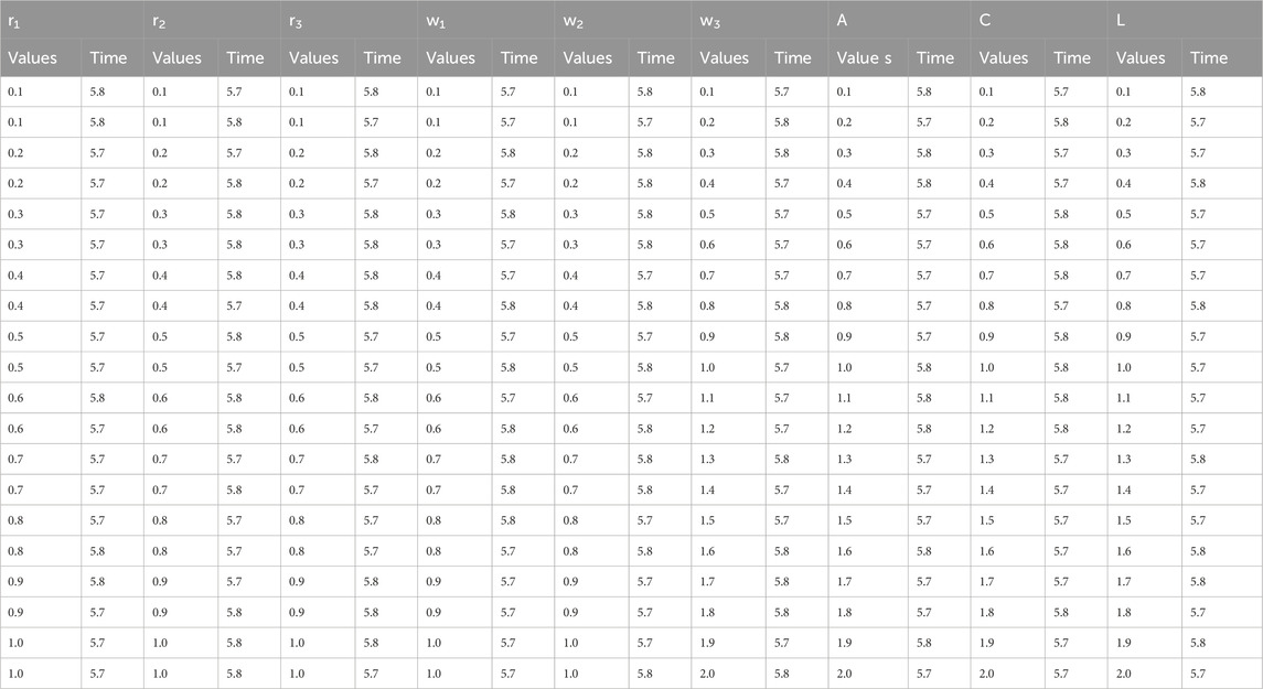
Table 7. Convergence time results for different values of AD-PO-guided WOA’s parameters.
Table 8 provides a statistical analysis of the convergence time results, listing measures of minimum, maximum, mean, standard deviation, and confidence intervals. This work gives a more detailed insight into the distribution and variation of convergence times under various parameter settings. One of the most important tasks of statistical metrics is to provide researchers with indications of the regularity and stability of such estimates that allow making adequate decisions in the optimization of the algorithms.
• Consistency: The mean convergence time is 5.072 s with a standard deviation of 0.9194 s.
• Confidence Interval: The 95% confidence interval ranges from 4.642 to 5.502 s, indicating reliable estimates.
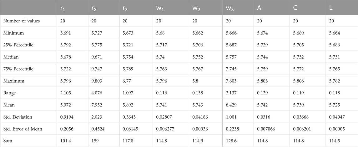
Table 8. Statistical analysis for the convergence time results for different values of AD-PO-guided WOA’s parameters.
In Table 9, an ANOVA test (Djaafari et al., 2022) is used to determine whether the differences in convergence times based on changes in the parameter values are significant. This type of statistical analysis aids in ascertaining if some parameter setting is significantly delaying the convergence time. With the analysis of ANOVA results, the researchers can easily see the influential parameters.
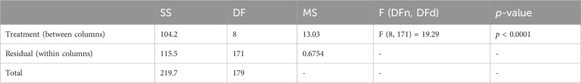
Table 9. ANOVA test for the Convergence Time Results for Different Values of AD-PO-Guided WOA’s Parameters.
Table 10 conducts a one-sample t-test (Abualigah and Ali, 2020; Muhammed Al-Kassab, 2022; Vankelecom et al., 2024) to compare convergence times to a theoretical mean of zero. This statistical analysis examines the statistical significance and size of differences in observed and anticipated convergence times. Through t-tests, the reliability of estimates of convergence time can be tested under different parameter settings and causes of variability or bias in the optimization process can be identified.
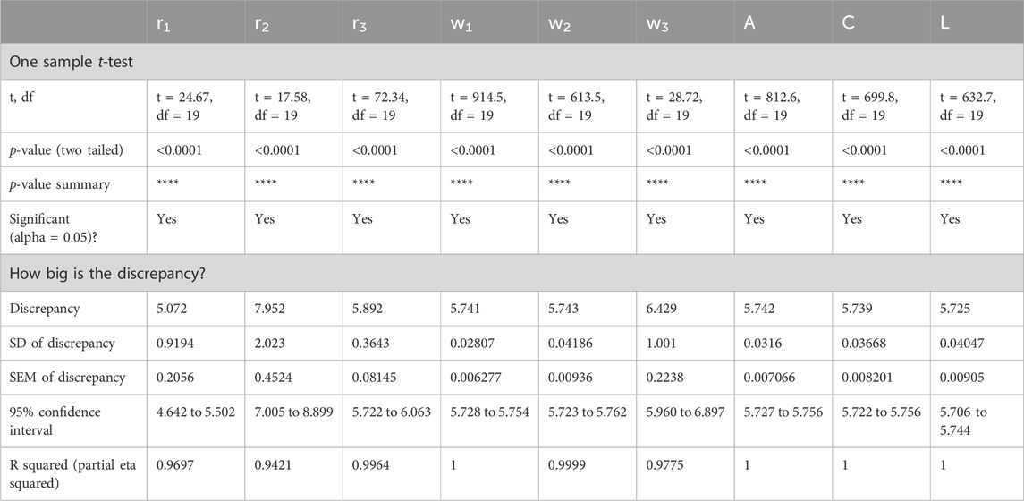
Table 10. One Sample t-test for the Convergence Time Results for Different Values of AD-PO-Guided WOA’s Parameters.
Minimization results are encapsulated in Table 11 for the AD-PO-Guided WOA algorithm at different parameter values. Analogy-based comparison and parameter-based comparison among different parameter combinations of the researchers to give the effectiveness of the algorithm in minimizing objective functions or fitness values. This table provides important information on the relationship between parameter settings and the level of depreciation achieved that helps in directing additional optimization attempts.
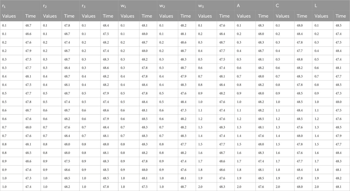
Table 11. Minimization results for different values of AD-PO-guided WOA’s parameters.
Table 12 provides a statistical summary of minimization results, comprising minimum, maximum, mean, standard deviation, and confidence intervals. This analysis gives an overall view of the distribution and variation of minimization outcomes under various parameter settings. Through these statistical measures, the consistency and dependability of minimization estimates can be evaluated, thus enabling well-informed decision-making in algorithm optimization.
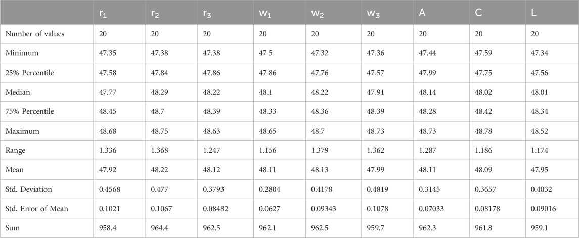
Table 12. Statistical analysis for the minimization results for different values of AD-PO-guided WOA’s parameters.
Table 13 performs an ANOVA test to assess whether the differences in minimization outcomes are statistically significant due to variations in parameter values. This statistical analysis is endorsed to identify which parameter settings have an important influence on the level of minimization reached. Relating to the ANOVA results, the researchers can prioritize the efforts of optimization of parameters that influence the algorithm’s effect in the minimization of the objective functions or fitness values.
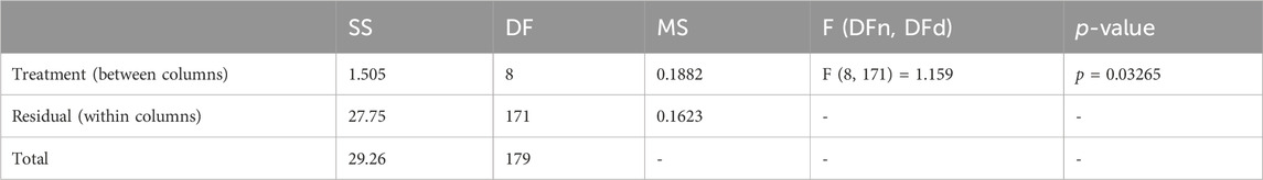
Table 13. ANOVA table for the Minimization Results for Different Values of AD-PO-Guided WOA’s Parameters.
Table 14 conducts one-sample t-tests to compare minimization outcomes with a theoretical mean of zero. This statistical analysis tests the statistical significance and the size of the differences between observed and expected minimization levels. Through conducting t-tests for each parameter setting, researchers can check the reliability of minimization estimates and also recognize potential sources of variability or bias in the optimization process. These results help in a better understanding of the performance of the algorithm and support the optimization efforts in the future.
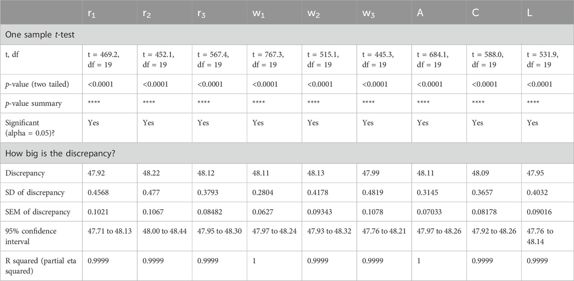
Table 14. One sample t-test for the Minimization Results for Different Values of AD-PO-Guided WOA’s Parameters.
Sensitivity analysis confirms the robustness of the AD-PO-Guided WOA algorithm. Optimal parameter tuning ensures quick convergence and effective minimization, highlighting the importance of sensitivity analysis in optimizing algorithm performance.
This current study will further highlight the combined feature of the Adaptive Dynamic Puma Optimizer (AD-PO) and Guided Whale Optimization Algorithm to investigate the performance of the optimized model proposed for the classification and forecasting of rainfall. The performance of the algorithm has been further evaluated in comparison with several existing documented methods present in the literature.
In the classification task, our algorithm of AD-PO-Guided WOA achieved excellent accuracy of 95.99%, significantly outperforming traditional classifiers like Random Forest (RF; 87.14%), Extreme Gradient Boosting (XGBoost; 83.95%), K-Nearest Neighbor (KNN; 82.38%), and Decision Tree (DT; 81.08%). The statistical significance of our algorithm’s performance was further proved by Wilcoxon’s rank-sum test to have a significant improvement over the others, holding a p-value of <0.05.
Conclusively, the MSE of the AD-PO-guided WOA-LSTM model in rainfall prediction was noticeably improved at 0.005078 compared to the baselines of ARIMA, at 0.02425, SARIMA, at 0.012407, and standard LSTM, at 0.013976. This corroborates a high predictive accuracy of our integrated method.
It is to be compared with some of the existing works like the AdaBoost algorithm with One versus All (OvA) SVM by Belghit et al., 2023, and several Neural Networks architectures by Barrera-Animas et al., 2022 which, apart from offering better accuracy satisfactorily, show far more robustness and reliability in conditions that constantly change. The intensive sensitivity studies and the results of Wilcoxon’s rank-sum test further confirm this inherent variability in the rainfall data. In general, the proposed AD-PO-Guided WOA algorithm enhanced the classification and forecasting accuracy of the rainfall, being useful for environmental and resource management applications. The improvement of the applicability of the model may also be increased in future work by incorporating more meteorological variables and broadening the geographical area using more rainfall gauge data.
Rainfall classification entails the systematic categorization and examination of different types of rainfall based on factors such as intensity, duration, distribution, and the associated meteorological conditions. Understanding these rainfall patterns and classifications is crucial across a spectrum of applications, including agriculture, water resource management, weather forecasting, and climate studies. The analysis of diverse aspects of rainfall aids in making well-informed decisions in areas like agricultural planning, efficient water resource utilization, precise weather predictions, and a deeper comprehension of climate-related phenomena. The potential of machine learning and metaheuristic algorithms becomes evident in their capacity to effectively address and overcome the challenges associated with rainfall classification. The paper introduces a novel algorithm named Adaptive Dynamic Puma Optimizer (AD-PO), which has been enhanced with the integration of the Guided Whale Optimization Algorithm (Guided WOA) for the specific purpose of rainfall classification. In the methodology, the dataset undergoes training using five distinct classifiers: Random Forest (RF), Extreme Gradient Boosting (XG Boost), K-Nearest Neighbor (KNN), and Decision Tree (DT). Subsequently, the proposed voting ensemble, the AD-PO-Guided WOA algorithm, consolidates predictions from these classifiers, employing a voting mechanism to select the predominant class. The effectiveness of the suggested AD-PO-Guided WOA algorithm is validated through a comparative analysis with other commonly utilized optimization algorithms documented in recent literature. Notably, the proposed voting algorithm exhibits superior performance metrics, achieving an accuracy of 94.11%, surpassing other voting classifiers. To validate the robustness of the proposed algorithms, rigorous assessments are conducted using statistical tests, including the Wilcoxon rank-sum test, along with detailed descriptive statistics.
For the future work in the context of rainfall classification and algorithmic advancement, there exist numerous pathways for prospective research and enhancements:
1. Optimization Refinement: Further refining the parameters of the proposed AD-PO-Guided WOA algorithm is imperative for enhancing its overall efficacy. Exploring additional metaheuristic techniques or amalgamating diverse algorithms has the potential to expedite convergence and augment classification accuracy.
2. Incorporation of Novel Features: Enriching the algorithm’s capabilities by integrating novel meteorological features or alternative data sources is a promising avenue. Adapting the algorithm to evolving meteorological conditions, especially in the context of climate change, is essential for its continued relevance.
3. Real-Time Adaptation: Adapting the algorithm for real-time applications, particularly in domains with time-sensitive requirements like weather forecasting, is paramount. This necessitates optimizing the algorithm for efficiency and scalability to handle substantial datasets and provide timely predictions.
4. Comprehensive Robustness Testing: Undertaking thorough robustness testing across various conditions, including extreme weather events and diverse geographical regions, is pivotal. Such testing offers insights into the algorithm’s reliability and generalizability, ensuring its applicability in diverse real-world scenarios.
5. Enhanced Explainability and Interpretability: The development of methodologies to interpret and elucidate the decision-making process of the algorithm is advantageous, especially in applications where transparency and interpretability are crucial. A clear understanding of the algorithm’s reasoning behind specific classifications can foster trust and facilitate broader adoption.
6. Diversification into Other Domains: Investigating the adaptability of the AD-PO-Guided WOA algorithm beyond rainfall classification is worthwhile. Evaluating its performance in various fields such as environmental monitoring, ecological studies, or any domain with analogous classification challenges can uncover its versatility.
7. Collaboration with Subject Matter Experts: Engaging in collaborations with experts in meteorology, hydrology, and related domains can offer valuable insights and domain-specific knowledge. Integrating this expertise into the algorithm’s development process can contribute to the creation of more accurate and contextually relevant models.
8. Regular Benchmarking against Leading Models: Consistently benchmarking the algorithm against the latest state-of-the-art models is vital for assessing its competitiveness. Staying abreast of advancements in machine learning and optimization techniques will serve as a guide for future enhancements.
The original contributions presented in the study are included in the article/Supplementary material, further inquiries can be directed to the corresponding authors.
E-SE-K: Writing–original draft, Writing–review and editing. AA: Writing–original draft, Writing–review and editing. ME: Writing–original draft, Writing–review and editing. AI: Writing–original draft, Writing–review and editing.
The author(s) declare financial support was received for the research, authorship, and/or publication of this article. Princess Nourah bint Abdulrahman University Researchers Supporting Project number (PNURSP2024R308), Princess Nourah bint Abdulrahman University, Riyadh, Saudi Arabia.
The authors declare that the research was conducted in the absence of any commercial or financial relationships that could be construed as a potential conflict of interest.
All claims expressed in this article are solely those of the authors and do not necessarily represent those of their affiliated organizations, or those of the publisher, the editors and the reviewers. Any product that may be evaluated in this article, or claim that may be made by its manufacturer, is not guaranteed or endorsed by the publisher.
Abdollahzadeh, B., Khodadadi, N., Barshandeh, S., Trojovský, P., Soleimanian Gharehchopogh, F., El-kenawy, E.-S. M., et al. (2024). Puma optimizer (PO): a novel metaheuristic optimization algorithm and its application in machine learning. January: Cluster Computing.
Abualigah, L., and Ali, D. (2020). A comprehensive survey of the grasshopper optimization algorithm: results, variants, and applications. Neural Comput. Appl. 32 (19), 15533–15556. doi:10.1007/s00521-020-04789-8
Alkhammash, E. H., Assiri, S. A., Nemenqani, D. M., Althaqafi, R. M., Hadjouni, M., Saeed, F., et al. (2023). Application of machine learning to predict COVID-19 spread via an optimized BPSO model. Biomimetics 8 (6), 457. doi:10.3390/biomimetics8060457
Alkhammash, E. H., Hadjouni, M., and Elshewey, A. M. (2022). A hybrid ensemble stacking model for gender voice recognition approach. Electronics 11 (11), 1750. doi:10.3390/electronics11111750
Appiah-Badu, N. K. A., Missah, Y. M., Amekudzi, L. K., Ussiph, N., Frimpong, T., and Ahene, E. (2022). Rainfall prediction using machine learning algorithms for the various ecological zones of Ghana. IEEE Access 10, 5069–5082. doi:10.1109/access.2021.3139312
Avanzato, R., Beritelli, F., Raspanti, A., and Russo, M. (2020). Assessment of multimodal rainfall classification systems based on an audio/video dataset. Int. J. Adv. Sci. Eng. Inf. Technol. 10, 1163–1168. doi:10.18517/ijaseit.10.3.12130
Bahraoui, Z., Bahraoui, F., and Bahraoui, M. (2018). Modeling wind energy using copula. Open Access Libr. J. 5, 1–14. doi:10.4236/oalib.1104984
Barrera-Animas, A. Y., Oyedele, L. O., Bilal, M., Akinosho, T. D., Delgado, J. M. D., and Akanbi, L. A. (2022). Rainfall prediction: a comparative analysis of modern machine learning algorithms for time-series forecasting. Mach. Learn. Appl. 7, 100204. doi:10.1016/j.mlwa.2021.100204
Belghit, A., Lazri, M., Ouallouche, F., Labadi, K., and Ameur, S. (2023). Optimization of One versus All-SVM using AdaBoost algorithm for rainfall classification and estimation from multispectral MSG data. Adv. Space Res. 71, 946–963. doi:10.1016/j.asr.2022.08.075
Benali, F., Bodénès, D., Labroche, N., and de Runz, C. (2021). MTCopula: synthetic complex data generation using copula. Int. Workshop Data Warehous. OLAP.
Breidablik, H. J., Lysebo, D. E., Johannessen, L., Skare, Å., Andersen, J. R., and Kleiven, O. (2020). Effects of hand disinfection with alcohol hand rub, ozonized water, or soap and water: time for reconsideration? J. Hosp. Infect. 105 (2), 213–215. doi:10.1016/j.jhin.2020.03.014
Chen, M., Vincent Poor, H., Saad, W., and Cui, S. (2021). Convergence time optimization for federated learning over wireless networks. IEEE Trans. Wirel. Commun. 20 (4), 2457–2471. doi:10.1109/twc.2020.3042530
Chen, T., He, T., Benesty, M., Khotilovich, V., Tang, Y., Cho, H., et al. (2015). Xgboost: extreme gradient boosting. R. package version 0 1 (4), 1–4.
Classification Scenario (2024). GitHub. Available at: https://github.com/SayedKenawy/Rainfall-Final-Project.
Cru, T. S. (2024). Version 4.02 google earth interface. CRU TS V. 4.02 Google Earth Interface. Available at: https://crudata.uea.ac.uk/cru/data/hrg/cru_ts_4.02/ge/(Accessed January 3, 2024).
Djaafari, A., Ibrahim, A., Bailek, N., Bouchouicha, K., Hassan, M. A., Kuriqi, A., et al. (2022). Hourly predictions of direct normal irradiation using an innovative hybrid LSTM model for concentrating solar power projects in hyper-arid regions. Energy Rep. 8 (November), 15548–15562. doi:10.1016/j.egyr.2022.10.402
El-Kenawy, E. S. M., Ibrahim, A., Mirjalili, S., Eid, M. M., and Hussein, S. E. (2020). Novel feature selection and voting classifier algorithms for COVID-19 classification in CT images. IEEE access 8, 179317–179335. doi:10.1109/access.2020.3028012
Ghoneim, S. S., Farrag, T. A., Rashed, A. A., El-Kenawy, E. S. M., and Ibrahim, A. (2021). Adaptive dynamic meta-heuristics for feature selection and classification in diagnostic accuracy of transformer faults. Ieee Access 9, 78324–78340. doi:10.1109/access.2021.3083593
Harris, I., Jones, P. D., Osborn, T. J., and Lister, D. H. (2014). Updated high-resolution grids of monthly climatic observations - the CRU TS3.10 Dataset. Int. J. Climatol. 34, 623–642. doi:10.1002/joc.3711
Hassan, M. A., Bailek, N., Bouchouicha, K., Ibrahim, A., Jamil, B., Kuriqi, A., et al. (2022). Evaluation of energy extraction of PV systems affected by environmental factors under real outdoor conditions. Theor. Appl. Climatol. 150, 715–729. doi:10.1007/s00704-022-04166-6
Hazarika, B. B., and Gupta, D. (2020). Modelling and forecasting of COVID-19 spread using wavelet-coupled random vector functional link networks. Appl. Soft Comput. 96, 106626. doi:10.1016/j.asoc.2020.106626
Jeong, C. H., and Yi, M. Y. (2023). Correcting rainfall forecasts of a numerical weather prediction model using generative adversarial networks. J. Supercomput. 79 (2), 1289–1317. doi:10.1007/s11227-022-04686-y
Khadartsev, A. A., Eskov, V. V., Pyatin, V. F., and Filatov, M. A. (2021). The use of tremorography for the assessment of motor functions. Biomed. Eng. 54 (6), 388–392. doi:10.1007/s10527-021-10046-6
Khafaga, D., Alhussan, A., El-kenawy, E.-S., Ibrahim, A., Said, H., El-Mashad, S., et al. (2022a). Improved prediction of metamaterial antenna bandwidth using adaptive optimization of LSTM. Comput. Mater. Continua 73 (1), 865–881. doi:10.32604/cmc.2022.028550
Khafaga, D., Alhussan, A., El-kenawy, E.-S., Takieldeen, A., Hassan, T., Hegazy, E., et al. (2022b). Meta-heuristics for feature selection and classification in diagnostic breast cancer. CMC 73, 749–765. doi:10.32604/cmc.2022.029605
Lazri, M., Labadi, K., Brucker, J. M., and Ameur, S. (2020). Improving satellite rainfall estimation from MSG data in Northern Algeria by using a multi-classifier model based on machine learning. J. Hydrology 584, 124705. doi:10.1016/j.jhydrol.2020.124705
Li, R. H., and Belford, G. G. (2002). “Instability of decision tree classification algorithms,” in Proceedings of the eighth ACM SIGKDD international conference on Knowledge discovery and data mining, 570–575.
Mirjalili, S., Mirjalili, S. M., Saremi, S., and Mirjalili, S. (2020). Whale optimization algorithm: theory, literature review, and application in designing photonic crystal filters. Nature-inspired Optim. Theor. literature Rev. Appl., 219–238. doi:10.1007/978-3-030-12127-3_13
Muhammed Al-Kassab, M. (2022). The use of one sample T-test in the real data. J. Adv. Math. 21, 134–138. doi:10.24297/jam.v21i.9279
Nazir, M. S., Alturise, F., Alshmrany, S., Nazir, H. M. J., Bilal, M., Abdalla, A. N., et al. (2020). Wind generation forecasting methods and proliferation of artificial neural network: a review of five years research trend. Sustainability 12 (9), 3778. doi:10.3390/su12093778
Ni, L., Wang, D., Singh, V. P., Wu, J., Wang, Y., Tao, Y., et al. (2020). Streamflow and rainfall forecasting by two long short-term memory-based models. J. Hydrology 583, 124296. doi:10.1016/j.jhydrol.2019.124296
Osman, A. I. A., Ahmed, A. N., Chow, M. F., Huang, Y. F., and El-Shafie, A. (2021). Extreme gradient boosting (Xgboost) model to predict the groundwater levels in Selangor Malaysia. Ain Shams Eng. J. 12 (2), 1545–1556. doi:10.1016/j.asej.2020.11.011
Pal, A. K., Kamal, S., Krishna Nagar, S., Bandyopadhyay, B., and Fridman, L. (2020). Design of controllers with arbitrary convergence time. Automatica 112 (February), 108710. doi:10.1016/j.automatica.2019.108710
Parmar, A., Katariya, R., and Patel, V. (2019). “A review on random forest: an ensemble classifier,” in International conference on intelligent data communication technologies and internet of things (ICICI) 2018 (Springer International Publishing), 758–763.
Patel, H. H., and Prajapati, P. (2018). Study and analysis of decision tree based classification algorithms. Int. J. Comput. Sci. Eng. 6 (10), 74–78. doi:10.26438/ijcse/v6i10.7478
Petropoulos, F., Apiletti, D., Assimakopoulos, V., Babai, M. Z., Barrow, D. K., Ben Taieb, S., et al. (2022). Forecasting: theory and practice. Int. J. Forecast. 38 (3), 705–871. doi:10.1016/j.ijforecast.2021.11.001
Praveen, B., Talukdar, S., Mahato, S., Mondal, J., Sharma, P., Islam, A. R. M. T., et al. (2020). Analyzing trend and forecasting of rainfall changes in India using non-parametrical and machine learning approaches. Sci. Rep. 10 (1), 10342. doi:10.1038/s41598-020-67228-7
Priyam, A., Abhijeeta, G. R., Rathee, A., and Srivastava, S. (2013). Comparative analysis of decision tree classification algorithms. Int. J. Curr. Eng. Technol. 3 (2), 334–337.
Raval, M., Sivashanmugam, P., Pham, V., Gohel, H., Kaushik, A., and Wan, Y. (2021). Automated predictive analytics tool for rainfall forecasting. Sci. Rep. 11 (1), 17704. doi:10.1038/s41598-021-95735-8
Ridwan, W. M., Sapitang, M., Aziz, A., Kushiar, K. F., Ahmed, A. N., and El-Shafie, A. (2021). Rainfall forecasting model using machine learning methods: case study Terengganu, Malaysia. Ain Shams Eng. J. 12, 1651–1663. doi:10.1016/j.asej.2020.09.011
Rizk, F. H., Arkhstan, S., Zaki, A. M., Kandel, M. A., and Towfek, S. K. (2023). Integrated CNN and waterwheel plant algorithm for enhanced global traffic detection. J. Artif. Intell. Metaheuristics 6, 36–45. doi:10.54216/jaim.060204
Rodriguez-Galiano, V. F., Ghimire, B., Rogan, J., Chica-Olmo, M., and Rigol-Sanchez, J. P. (2012). An assessment of the effectiveness of a random forest classifier for land-cover classification. ISPRS J. photogrammetry remote Sens. 67, 93–104. doi:10.1016/j.isprsjprs.2011.11.002
Saha, A., Singh, K. N., Ray, M., and Rathod, S. (2020). A hybrid spatio-temporal modelling: an application to space-time rainfall forecasting. Theor. Appl. Climatol. 142, 1271–1282. doi:10.1007/s00704-020-03374-2
Samee, N., El-Kenawy, E.-S., Atteia, G., Jamjoom, M., Ibrahim, A., Abdelhamid, A., et al. (2022). Metaheuristic optimization through deep learning classification of COVID-19 in chest X-ray images. CMC 73, 4193–4210. doi:10.32604/cmc.2022.031147
Suguna, N., and Thanushkodi, K. (2010). An improved k-nearest neighbor classification using genetic algorithm. Int. J. Comput. Sci. Issues 7 (2), 18–21.
Tarek, Z., Shams, M. Y., Elshewey, A. M., El-kenawy, E. S. M., Ibrahim, A., Abdelhamid, A. A., et al. (2023). Wind power prediction based on machine learning and deep learning models. Comput. Mater. Continua 75 (1), 715–732. doi:10.32604/cmc.2023.032533
Vankelecom, L., Loeys, T., and Moerkerke, B. (2024). How to safely reassess variability and adapt sample size? A primer for the independent samples t test. Adv. Methods Pract. Psychol. Sci. 7 (1), 25152459231212128. doi:10.1177/25152459231212128
Keywords: environmental issues, rainfall, guided whale optimization algorithm, adaptive dynamic puma optimizer, voting ensemble, forecasting, classification
Citation: Elkenawy E-SM, Alhussan AA, Eid MM and Ibrahim A (2024) Rainfall classification and forecasting based on a novel voting adaptive dynamic optimization algorithm. Front. Environ. Sci. 12:1417664. doi: 10.3389/fenvs.2024.1417664
Received: 15 April 2024; Accepted: 06 June 2024;
Published: 26 June 2024.
Edited by:
Linlin Xu, University of Waterloo, CanadaReviewed by:
Barenya Bikash Hazarika, Assam Down Town University, IndiaCopyright © 2024 Elkenawy, Alhussan, Eid and Ibrahim. This is an open-access article distributed under the terms of the Creative Commons Attribution License (CC BY). The use, distribution or reproduction in other forums is permitted, provided the original author(s) and the copyright owner(s) are credited and that the original publication in this journal is cited, in accordance with accepted academic practice. No use, distribution or reproduction is permitted which does not comply with these terms.
*Correspondence: El-Sayed M. Elkenawy, c2tlbmF3eUBpZWVlLm9yZw==; Amel Ali Alhussan, YWFhbGh1c3NhbkBwbnUuZWR1LnNh
Disclaimer: All claims expressed in this article are solely those of the authors and do not necessarily represent those of their affiliated organizations, or those of the publisher, the editors and the reviewers. Any product that may be evaluated in this article or claim that may be made by its manufacturer is not guaranteed or endorsed by the publisher.
Research integrity at Frontiers
Learn more about the work of our research integrity team to safeguard the quality of each article we publish.