Fast dynamic prediction of consequences of heavy gas leakage accidents based on machine learning

The field of emergency risk management in chemical parks has been characterized by a lack of fast, precise and dynamic prediction methods. The application of computational fluid dynamics (CFD) models, which offer the potential for dynamic and precise prediction, has been hindered by high computational costs. Therefore, taking liquid benzene as a case study, this paper combined machine learning (ML) algorithms with a CFD-based precise prediction model, to develop an ML model for fast dynamic prediction of heavy gas leakage consequences in chemical parks. Employing the CFD data as the input, the prediction models were developed using ML algorithms, refined with Bayesian optimization for parameter tuning. This study utilized PHOENICS software to establish a dynamic prediction model for the diffusion of liquid benzene leakage, validated by Burro nine experiment data. Comparative analyses of models based on five ML algorithms were conducted to evaluate the reliability of their predictions using both CFD standard and noisy data. The results indicated that temperature had the most significant effect on the consequences of the leakage accidents among four key factors (wind speed, temperature, leakage aperture and atmospheric stability), followed by wind speed. These factors served as input variables for ML model training. Among the models evaluated, the eXtreme Gradient Boosting (XGBoost) model showed superior performance, irrespective of the presence of noise in the data. An XGBoost-based fast prediction model was ultimately developed for predicting the consequences of liquid benzene leakage. A case analysis was conducted to validate the feasibility of the model prediction. The relative errors between the predicted and actual values of the model for acute exposure guideline level-1 (AEGL-1), AEGL-2, and AEGL-3 distances were 2.70%, 2.58%, and 0.23%, respectively. Furthermore, the XGBoost model completed the prediction in only 0.218 s, a stark contrast to the hours necessitated by the CFD model, thus offering substantial computational time savings while maintaining high accuracy levels. This paper introduces an ML model for fast dynamic prediction of heavy gas leakage, enabling chemical parks to make more timely and accurate decisions in emergency risk management.

1 Introduction

Recent years have witnessed a marked increase in safety accidents globally, leading to significant loss of life and property damage, and severely impacting the chemical industry (Kang et al., 2017). These accidents are primarily attributed to shortcomings in risk management techniques, such as insufficient monitoring systems and emergency response capabilities, hindering effective risk detection and management (Liu and Li, 2013). In response, government regulations are escalating their safety management requirements for enterprises, with a particular focus on enhancing emergency response technologies in the chemical industry. Consequently, the advancement and integration of information technology, the Internet of Things, big data, and artificial intelligence (AI) are facilitating the development of smart chemical parks (Li et al., 2017). The application of modern technologies for early warnings and precise prediction of potential risks becomes imperative (Wang et al., 2017; Chai et al., 2023), which is essential for fostering the establishment and growth of smart chemical parks (Kang et al., 2017).

Model-driven methods, including the SLAB, AFTOX, ALOHA, and PHAST models, have long been prevalent for analyzing the consequences of heavy gas leakage accidents (Zhang et al., 2007). Multiple studies (Li et al., 2019; Terzioglu and Iskender, 2021; Barjoee et al., 2022; Cheng et al., 2022) have used these models to determine the impact ranges of different hazardous accidents. While these models are computationally convenient and time efficient, their reliance on static assumptions limits their application in the dynamic environment of smart chemical parks. More recent advancements have seen the application of models using the MATLAB language (Bu et al., 2022; Liu and Wang, 2022) and computational fluid dynamics (CFD) software (Wu et al., 2024; Zhou et al., 2024), which offer refined simulations of leakage diffusion by providing time-specific concentration distributions. Nevertheless, the complexity and extensive computational time of these numerical models (Wang et al., 2019) limit their application in emergency response scenarios (Pan and Jiang, 2004). Therefore, there is a crucial need for a prediction model that can combine dynamic simulation capabilities with fast response to fulfill the real-time prediction requirements in smart parks.

Data-driven methods, encompassing both statistical and machine learning (ML) models, offer robust data processing and learning capabilities for predicting pollutant concentrations (Zhu L. et al., 2023; Fu et al., 2023). These methods excel in identifying statistical patterns and providing fast and efficient predictions. While data-driven methods analyze data to predict trends from historical patterns, their assumption of linear relationships often fails to capture the complex, nonlinear dynamics present in environmental data (Arsic et al., 2020; Lu et al., 2020), leading to less accurate predictions (Zhang et al., 2018). In contrast, Ahmed et al. (2020) demonstrated that ML models were better suited to handle the complex characteristics of pollutant data, such as nonlinearity, periodicity, and seasonality. Fang et al. (2019) compared a multilayer perceptron (MLP) model with a linear regression model using meteorological observations, PM_2.5 concentrations, and air quality index (AQI), finding the MLP model to be more accurate. Furthermore, ensemble learning (EL) has also been extensively investigated for predicting pollutant concentrations. Wang et al. (2021) analyzed pollutant emission data and meteorological observations, including wind speed, direction, temperature, and atmospheric pressure. They compared the effectiveness of various ML algorithms—MLP, Decision Tree (DT), Support Vector Machine (SVM), eXtreme Gradient Boosting (XGBoost), Light Gradient Boosting Machine (LightGBM), and Stacking—in predicting the impact of air pollution in the park. Based on the prediction performance of different algorithms, the more stable Stacking model, noted for its stability, was ultimately selected to ensure reliable prediction support for enterprises. Further, Zhu J. Y. et al. (2023) examined models for ground-level ozone concentration prediction using LightGBM, Random Forest (RF), SVM and Recurrent Neural Network (RNN) algorithms, leveraging pollutant concentrations and meteorological observations. The LightGBM model outperformed its counterparts, with R² of 0.92. These studies underscore the importance of diverse input data, including environmental, satellite remote sensing, and time-series data, as well as meteorological variables such as temperature, wind speed, direction, and humidity. Finally, a variety of mainstream algorithms, such as MLP, DT, RF, XGBoost, and LightGBM, were used to construct and compare prediction models (Kang et al., 2020; Chen et al., 2022). Currently, scholars worldwide have focused on employing data-driven methods in AQI studies to predict pollutant concentrations (Ma et al., 2022; Peng et al., 2023). However, the application of these techniques for predicting the risks associated with accidents remains less explored, primarily due to the reliance of pollutant concentration predictions on extensive monitoring data, in contrast to the limited data for accident risk prediction.

To improve risk prediction and overcome the challenges of not having easy access to observational data, some researchers (So et al., 2010; Wang et al., 2015; Qiu et al., 2017) initially trained ML models using real-time monitoring data to predict concentrations of hazardous gas leakage. However, due to considerable measurement inaccuracies, these predictions proved suboptimal. Currently, a methodology that integrates model-driven and data-driven methods has been employed for predicting pollutant concentrations. This method employs the CFD model to generate extensive input datasets. Ni et al. (2020) utilized simulation data from Fluent software to develop a deep learning-based model that accurately predicted the diffusion concentrations of toxic heavy gas. Jiao et al. (2021) constructed a quantitative consequence prediction model based on a toxic diffusion database derived from PHAST software simulations. RF, XGBoost and Deep Neural Network (DNN) algorithms were implemented and compared to identify the best performance method for model construction. Wang et al. (2023) formulated a leakage model for liquid ammonia storage tanks using PHAST software, considering factors such as atmospheric stability, wind speed, and leakage aperture. Six models were compared, including linear regression, K-Nearest Neighbor (KNN), AdaBoost, DT, RF, and XGBoost. The emergency response model of liquid ammonia leakage was ultimately developed based on the XGBoost algorithm. Additionally, some researchers (Wang et al., 2015; Qiu et al., 2018) employed artificial neural networks trained on the PHAST model and utilized particle swarm optimization (PSO) algorithms to predict the diffusion of hazardous gases. These methods were investigated with the aim of overcoming the prevailing challenges of achieving both high accuracy and prediction efficiency simultaneously. Despite these advancements, existing risk prediction research has certain deficiencies. Specifically, the dynamic process of hazardous chemical evaporation is often disregarded. Therefore, in this study, the CFD model was used to develop a dynamic model for heavy gas leakage diffusion and to evaluate the impact of various factors on accident consequences. Furthermore, while standard data from numerical simulations are commonly used, real-world data typically contain noise (Li X. et al., 2021; Liu et al., 2023), challenging the accuracy of ML-based prediction models when working with such data. The reliability of ML prediction models in handling noisy data remains an area requiring further investigation. Five algorithms—MLP, DT, RF, XGBoost, LightGBM—were selected to develop prediction models, which were systematically evaluated for their performance using both CFD standard and noisy data. Additionally, the prediction time of these models was compared to provide faster and more accurate gas diffusion prediction with the CFD model. The objective of these advancements is to enhance environmental risk management and mitigation efforts.

Section 2 of this paper introduces the scenario and simulation scheme for a heavy gas leakage accident, the selected ML algorithms and the modelling process, and confirms the reliability of the CFD model in simulating heavy gas leakage. Section 3 analyzes the influencing factors, correlation between variables and diffusion mechanism of the consequences of the leakage accidents. It evaluates the ML models based on standard data and noisy data respectively, and identifies the most effective model for predictive analysis. Section 4 summarizes the research and the shortcomings of this study.

2 Materials and methods

2.1 Heavy gas leakage scenarios and simulation schemes

2.1.1 Characteristics and hazardous of benzene

Benzene at ambient temperature is a colorless and transparent fluid characterized by a density of approximately 880 kg/m³. The saturated vapor pressure of liquid benzene demonstrates variation across different temperatures (Figure 1). Prolonged or high levels of exposure to liquid benzene can adversely affect health. A leakage resulting in the inhalation of benzene vapor can lead to symptoms such as headache, dizziness, drowsiness, causing severe neurological and liver damage, and being potentially fatal. Therefore, this paper aims to investigate the phenomenon of benzene leakage by developing a prediction model for the concentration and diffusion of heavy gas leakage.

Figure 1

Figure 1. The saturated vapor pressure of liquid benzene varies with temperature.

2.1.2 Classification of hazardous distances

The standard concentrations of Acute Exposure Guideline Levels (AEGLs), established by the US National Advisory Committee (NAC), were utilized to determine hazardous distances. AEGLs apply to the adverse effects associated with short-duration and sudden-onset chemical leakages (Zhao and Chen, 2014). AEGLs are categorized into three levels: AEGL-1, AEGL-2 and AEGL-3. Each level corresponds to a specific level of acute toxicity. Under these standards, AEGL-1, AEGL-2 and AEGL-3 thresholds, corresponding to the 10-min liquid benzene leakage, are 420 mg/m³, 6,500 mg/m³ and 31,000 mg/m³, respectively. The concentration limits associated with specific injury symptoms are outlined in Table 1.

Table 1

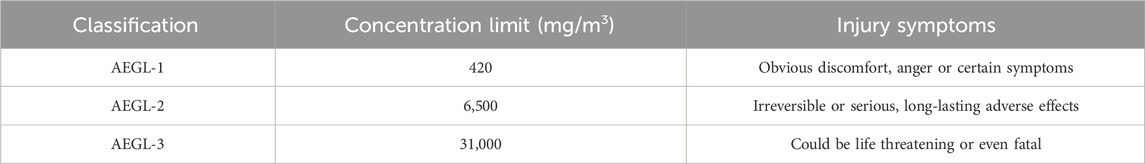
Table 1. AEGLs for the 10-min leakage of liquid benzene.

2.1.3 Assumptions for accident scenario

This study examined an accident scenario involving a liquid benzene storage tank located within a chemical park. The tank, characterized by its horizontal orientation and a capacity of 135 m³, was maintained under ambient temperature and pressure conditions. The tank suffered a rupture due to the impact of an external object, forming a circular breach approximately 0.5 m above the ground, encircled by a 35 m radius cofferdam. Additionally, the internal and external factors that influence tank leakage are crucial to the study of gas leakage diffusion. Zhu et al. (2009) and Sun and Guo (2010) have discussed the significant effects of wind speed and atmospheric stability on gas diffusion. A summary of the current status of domestic and international research on leakage diffusion has been provided, and it has been demonstrated that leakage aperture, temperature and wind speed were important factors affecting gas diffusion (Zhou et al., 2012). Furthermore, Wang et al. (2023) constructed a liquid ammonia leakage prediction model based on environmental factors such as atmospheric stability, wind speed, and leakage aperture. Therefore, a range of values was selected for four factors: leakage aperture, wind speed, temperature, and atmospheric stability. These values are presented in Supplementary Table S2. The apertures considered were 100 mm 150 mm and 200 mm; wind speed ranged from 1 m/s to 6 m/s in 1 m/s increments. Temperatures were set at 20°C, 25°C, 30°C, 40°C and 50°C. Atmospheric stabilities were categorized as unstable, neutral and stable. The duration of leakage was set at 10 min. In total, 270 different scenarios were simulated, with the fundamental parameters of the leakage tank detailed in Supplementary Table S3.

The leakage rate of liquid benzene after a leakage is calculated using the Bernoulli Eq. 1 (Fu, 2008):

$Q_L=C_{d}A\rho \sqrt{\frac{2\left(P-P_0\right)}{\rho }+2gh}(1)$

where $Q_L$ represents the rate of liquid leakage, kg/s. $C_d$, the liquid leakage coefficient, is taken as 0.65. $A$ denotes the area of rupture, m². $\rho$ signifies the density of the liquid, kg/m³. $P$ and $P_0$ are the internal and ambient pressures, respectively, Pa. $g$ represents the gravity acceleration at 9.81 m/s². $h$ indicates the height of the liquid level above the rupture, m. Given that liquid benzene was stored at ambient conditions, where both the storage and ambient temperatures remained below its boiling point, flash and heat evaporation processes were precluded. This scenario led to the formation of a liquid pool on the ground. The subsequent evaporation of this pool was primarily driven by the air movement over its surface, and the mass evaporation rate is thus calculated as:

$Q_v=\alpha p\frac{M}{R{T}_0}{u}^{\frac{\left(2-n\right)}{\left(2+n\right)}}{r}^{\frac{\left(4+n\right)}{\left(2+n\right)}}(2)$

where $Q_v$ denotes the mass evaporation rate, kg/s. $\alpha$ and $n$ represent the atmospheric stability coefficients. $p$ specifies the vapor pressure at the surface of the liquid, Pa. $M$ is the molar mass of the chemical, kg/mol. $R$ stands for the gas constant, J/(mol·k). $T_0$ indicates the ambient temperature, K. $u$ refers to the ambient wind speed, m/s. $r$ is the radius of the liquid pool, m. The rate of mass evaporation varied dynamically with the radius of the liquid pool. In cases of the continuous leakage, the dynamics radius of the liquid pool, $r\left(t\right)$, as a function of time $t$, adhered to the following Eq. 3 (Nielsen et al., 1995). Ultimately, a CFD-based dynamic diffusion model of liquid benzene leakage has been developed. This model calculated the radius of the liquid pool and the corresponding evaporation rate per second throughout the 10-min leakage period under various environmental conditions.

$r\left(t\right)={\left(\frac{t}{\sqrt[3]{\frac{9\pi \rho }{32g{Q}_L}}}\right)}^{\frac{3}{4}}(3)$

2.2 Machine learning (ML) algorithms

2.2.1 Introduction to ML algorithms

(1) Multi-layer perceptron (MLP)

The Multi-Layer Perceptron (MLP), a form of feed-forward neural network, encompasses two main processes: forward and back propagation (Ehteram et al., 2022). During forward propagation, the input data is processed through the layers of network, guided by weights and biases, to generate the predicted output of the model layer by layer. Conversely, back propagation adjusts these parameters via gradient descent by computing the gradient of the loss function with respect to the weights and biases, thus refining predictions to more closely match the true values.

(2) Decision tree (DT)

The Decision Tree (DT), a tree-based methodology, can effectively capture nonlinear relationships and clearly illustrate the decision-making process of each feature within a structured tree format. Nonetheless, the DT model exhibits a high sensitivity to noisy data, which can be mitigated by employing a Random Forest model, which mitigates the impact of noise (Yu et al., 2019).

(3) Random Forest (RF)

The Random Forest (RF) model enhances efficacy and robustness by integrating multiple DTs into a strong evaluator. It operates by having each decision tree independently predict on the input data, with the final prediction being derived through a method of weighted averaging or voting, as represented by the Eq. 4 Breiman (2001):

$g\left(x\right)=f\left(x\right)+f_1\left(x\right)+f_2\left(x\right)+\cdots +f_n\left(x\right)(4)$

where $g\left(x\right)$ represents the aggregate prediction from each simple decision tree $f\left(x\right)$. In constructing each decision tree, the RF model mitigates noise and overfits by employing bootstrap sampling, which means drawing from the training set with replacement (Wu and Zhao, 2013).

(4) eXtreme gradient boosting (XGBoost)

The eXtreme Gradient Boosting (XGBoost) model represents an advanced implementation of gradient boosting algorithms and stands as a noteworthy component in the EL models, playing a pivotal role in ensemble learning (EL) models due to its efficacy in capturing complex and nonlinear interactions (Chen and Guestrin, 2016). The core of the XGBoost model is a gradient boosting framework that sequentially constructs an ensemble of weak learners, typically decision trees, to minimize a differentiable loss function. What sets XGBoost apart is its efficient handling of sparse data and missing values, an aspect crucial for robustness in real-world data applications. It incorporates a sparsity-aware algorithm for handling missing data and employs a weighted quantile sketch for efficient approximate tree learning. To enhance generalization and mitigate overfitting, the XGBoost model integrates specific regularization mechanisms, including L1 (Lasso regression) and L2 (Ridge regression) penalties. These regularization terms add a penalization component to the objective function, effectively controlling the complexity of the model. The main formulas for the XGBoost model are as follows Eqs 5–7:

$Objective\left(\mathrm{\Theta }\right)={\sum }_{i=1}^n\left(y_i,{\widehat{y}}_i\right)+{\sum }_{k=1}^K\mathrm{\Omega }\left(f_k\right)(5)$

$l\left(y_i,{\widehat{y}}_i\right)={\left(y_i-{\widehat{y}}_i\right)}^2(6)$

$\mathrm{\Omega }\left(f_k\right)=\gamma T_k+\frac{1}{2}\alpha {\displaystyle \sum _{j=1}^{T_k}}\left|w_{kj}\right|+\frac{1}{2}\lambda {\displaystyle \sum _{j=1}^{T_k}}{w}_{kj}^2(7)$

In formula (5), the first term, ${\sum }_{i=1}^n\left(y_i,{\widehat{y}}_i\right)$ aggregates the losses computed over all $n$ samples, where $l\left(y_i,{\widehat{y}}_i\right)$ measures the discrepancy between the predicted ${\widehat{y}}_i$ and the actual $y_i$ values, which is defined here as the square of the residuals. The second term, ${\displaystyle {\sum }_{k=1}^K}\mathrm{\Omega }\left(f_k\right)$, is the sum of regularization terms for $K$ weak learners, typically decision trees, to control the complexity of the model. The term $\gamma T_k$ adds a penalty proportional to the number of leaf nodes $T_k$ in the tree $k$, with $\gamma$ serving as a non-negative regularization parameter. This term restricts tree growth and aids in mitigating overfitting by penalizing excessive complexity. The expression $\frac{1}{2}\alpha {\displaystyle {\sum }_{j=1}^{T_k}}\left|w_{kj}\right|$ denotes the L1 regularization (Lasso), which imposes a penalty on the absolute values of the leaf weights $w_{kj}$. This promotes sparsity in the leaf weights, potentially reducing some to zero, thereby facilitating feature selection within the trees. Meanwhile, $\frac{1}{2}\lambda {\displaystyle {\sum }_{j=1}^{T_k}}{w}_{kj}^2$ signifies the L2 regularization on the leaf weights $w_{kj}$ of the tree, with $\lambda$ serving as the regularization coefficient.

(5) Light Gradient Boosting Machine (LightGBM)

The Light Gradient Boosting Machine (LightGBM) model, also an ML algorithm based on gradient boosting trees (Zhu J. Y. et al., 2023), employs an innovative histogram-based learning method that not only reduces computational complexity but also significantly enhances training efficiency on large datasets (Gao et al., 2020). By iteratively learning from gradient boosting trees, the LightGBM model consistently improves model performance, exhibiting robust generalization capabilities and effectiveness, particularly in addressing regression problems (Li Z. et al., 2021; Wei et al., 2021).

2.2.2 Data pre-processing and model setting

The typical workflow for applying ML models encompasses several critical steps (Bruha, 2000): data collection, data preprocessing, feature correlation analysis, parameter tuning, model training and validation.

This study generated various accident scenario hypotheses using the CFD model, with the CFD simulation data serving as the training datasets. For the accident scenario outlined in section 2.1.3, the CFD model was employed to simulate 270 different working conditions. This simulation generated concentration data at various downwind distances at 10-s intervals, culminating in a total of 515,160 datasets. The variables included in the analysis were time, leakage aperture, wind speed, temperature, atmospheric stability and downwind distance, with the concentration outcome (C1) serving as the target variable. These variables were normalized using Z-Score standardization. Atmospheric stability, a categorical variable, was converted into a numerical format using One-Hot encoding. Pearson correlation coefficient, designed by the letter ‘$P_c$’, was employed to quantify the linear relationships between the variables. The correlation coefficient between each pair of variables was calculated using the following formula (8) (Shaik et al., 2024). To assess the model performance, a subset featuring specific conditions—200 mm leakage aperture, 6 m/s wind speed, 50°C temperature, and stable atmospheric stability—was selected for validation. The remaining data was divided into an 80% training set and a 20% testing set. Moreover, Bayesian optimization and 10-fold cross-validation were applied for parameter tuning and model training. Table 2 displays the hyperparameter range domains for each model and the optimization results achieved by the algorithm.

$P_c=\frac{{\sum }_{i=1}^n\left(x_i-\overline{x}\right)\left(y_i-\overline{y}\right)}{\sqrt{{\sum }_{i=1}^n{\left(x_i-\overline{x}\right)}^2{\sum }_{i=1}^n{\left(y_i-\overline{y}\right)}^2}}(8)$

where $P_c$ is the correlation coefficient. $x_i$ and $y_i$ denote the values of the two variables. $\overline{x}$ and $\overline{y}$ represent the means of the two variables. $n$ signifies the number of samples.

Table 2

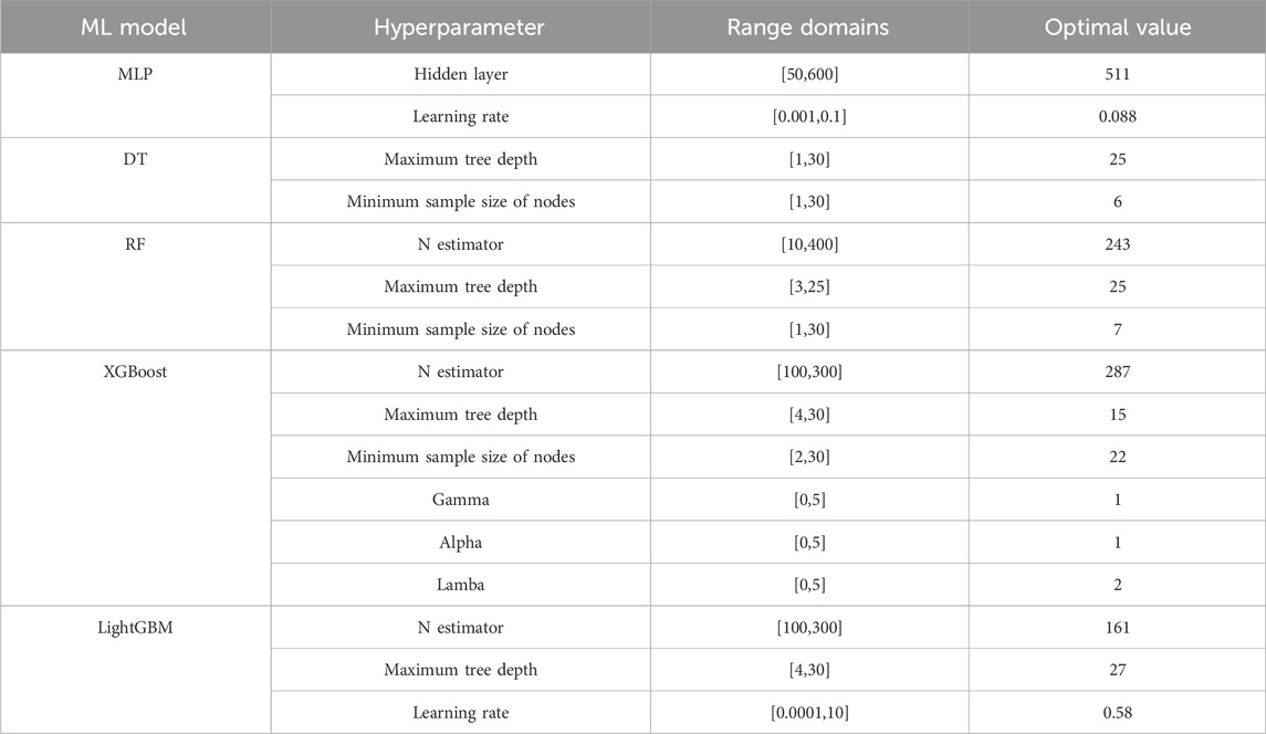
Table 2. Hyperparameter range domains of each model and results using Bayesian optimization.

To assess prediction accuracy for diffusion concentration within the ML algorithms, this study employed four principal metrics: the root mean square error (RMSE), mean absolute error (MAE), coefficient of determination (R²) and index of agreement (IOA). The formulas are as follows Eqs 9–12 (Shaik et al., 2022; Shaik et al., 2023; Shaik et al., 2024):

$RMSE=\sqrt{\frac{1}{n}{\displaystyle \sum _{i=1}^n}{\left(P_i-M_i\right)}^2}(9)$

$MAE=\frac{100\%}{n}{\displaystyle \sum _{i=1}^n}\left|\frac{P_i-M_i}{M_i}\right|(10)$

$R^2=1-\frac{{\displaystyle {\sum }_{i=1}^n}{\left(M_i-P_i\right)}^2}{{\displaystyle {\sum }_{i=1}^n}{\left(M_i-\overline{M_i}\right)}^2}(11)$

$IOA=1-\frac{{\displaystyle {\sum }_{i=1}^n}{\left(M_i-P_i\right)}^2}{{\displaystyle {\sum }_{i=1}^n}\left((\right|P_i-\overline{P_i}\left|+\right.|{\left.\left.M_i-\overline{M_i}\right|\right)}^2}(12)$

where $P_i$ represents the value predicted by the ML model. $M_i$ denotes the value simulated by the CFD model. $\overline{P_i}$ and $\overline{M_i}$ correspond to the mean of ML predicted values and CFD simulated values, respectively, with $n$ signifying the sample size.

2.3 CFD modelling and model validation

2.3.1 Selection of validation dataset

Before providing accurate sample data for ML models, it is necessary to validate the reliability of the CFD model in simulating the diffusion of heavy gas leakage. The purpose of this study is to validate the efficacy of the PHOENICS software in simulating heavy gas leakage, specifically through the application of the renowned Burro series experiments. These experiments took place in a circular water tank, measuring 58 m in diameter and 1 m in depth, where the liquefied natural gas (LNG) was released at a temperature of −164°C (Koopman et al., 1982). The significant temperature difference between the released LNG and surrounding environment facilitated the rapid vaporization of LNG, resulting in the formation of a cold and heavy gas cloud, approximately 1.5 times heavier than air (Yu et al., 2018). Methane concentrations were measured using sensors located at distances of 58 m, 140 m, 400 m and 800 m downwind from the release point. The initial conditions of the Burro series experiments are comprehensively outlined in Supplementary Table S4.

2.3.2 CFD modelling

(1) Physical model and governing equations

In this study, the computational domain was defined as 1,000 m × 300 m × 50 m. To enhance grid structure efficiency and minimize computational time, the domain was segmented into 200 × 100 × 25 using a gradient grid. The mesh independence analysis ensured that the CFD data remained consistent as the mesh size varied, as detailed in the Supplementary Text S1. Figure 2 illustrates the configuration of the detailed domain and grid setup within the CFD model. These modeling parameters were meticulously chosen to accurately simulate the heavy gas leakage scenario, laying a robust groundwork for subsequent analysis.

Figure 2

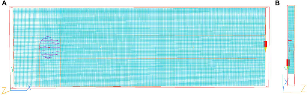
Figure 2. The configuration of the CFD model, focusing on: (A) model setting on the X-Z plane and (B) model setting on the Y-Z plane.

In this study, the Core module of the PHOENICS 6.0 software was used as the simulation platform. The turbulence model chosen was the widely used standard k-ε model within PHOENICS, with the specific equations given by Eqs 13, 14:

$\frac{\partial \left(\rho k\right)}{\partial t}+\frac{\partial \left(\rho u_{j}k\right)}{\partial x_j}=\frac{\partial }{\partial x_j}\left[\left(\mu +\frac{{\mu }_t}{{\sigma }_k}\right)\frac{\partial k}{\partial x_j}\right]+P_k-\rho \epsilon (13)$

$\frac{\partial \left(\rho \epsilon \right)}{\partial t}+\frac{\partial \left(\rho u_j\epsilon \right)}{\partial x_j}=\frac{\partial }{\partial x_j}\left[\left(\mu +\frac{{\mu }_t}{{\sigma }_{\epsilon }}\right)\frac{\partial \epsilon }{\partial x_j}\right]+{C_{1\epsilon }\frac{\epsilon }{k}P}_k-C_{2\epsilon }\rho \frac{{\epsilon }^2}{k}(14)$

where ${\mu }_t$ denotes the turbulent viscosity, kg/(m·s). $u_j$ indicates the velocity component in the $j$-direction, m/s, and $x_j$ corresponds to the spatial coordinate in that direction, m. $\mu$ is the molecular viscosity, kg/(m·s). ${\sigma }_k$ and ${\sigma }_{\epsilon }$ are the Prandtl numbers associated with turbulence kinetic energy $k$ and dissipation rate $\epsilon$, respectively, with their values set at ${\sigma }_k$ = 1.0 and ${\sigma }_{\epsilon }$ = 1.3. $P_k$ is the turbulence kinetic energy production term generated by the mean velocity gradient, m²/s³. $C_{1\epsilon }$ and $C_{2\epsilon }$ represent empirical constants taken as 1.44 and 1.92, respectively.

(2) Physical Properties

In the Properties section, set the ambient temperature to 35.4°C and the atmospheric pressure to 101,325 Pa. The Inverse Linear option was selected for the density setting to configure the density of the methane-air mixture, thereby accurately simulating the settling process of heavy gas, incorporating the impact of gravity was vital. Additionally, activate the gravity option Density Difference and set the gravitational acceleration to −9.81 m/s² in the Z direction.

(3) Boundary condition settings

The inlet boundary conditions of the model utilized the Wind property to define wind speed and direction. The index method ensured an accurate representation of the vertical gradient change in wind speed (Li and Tian, 2011). Given that the Burro series experiments were conducted in an open area without obvious obstacles, the effective roughness height in this study was set at 0.0002 m, and the wind profile index was chosen as 0.16.

(4) Inlet settings

A series of Inlet objects were selected to simulate the evaporation rates from the liquid pool. The leakage scenario was simplified to model the complete evaporation of LNG from a 58 m diameter liquid pool. The evaporation rate was approximated as the leakage rate, with the Mass Flow of the Inlet object set to 24.2 m³/min. Additionally, the solver variable C1 was added into the Models section, assigning a value of 1.0. The results of C1 were extracted after the completion of simulation and converted to the concentration of methane (CH₄) using calculation formula (15):

$C_{{CH}_4}=C1\times {\rho }_a\times {10}^6(15)$

where $C_{{CH}_4}$ represents the concentration of CH₄, mg/m³.

2.3.3 CFD simulation validation

The Burro nine experiment was selected to evaluate the accuracy of the CFD model in simulating the diffusion of heavy gas leakage. Figure 3 illustrates the concentration distribution of the gas cloud at T = 80 s for the Burro nine experiment across two planes. Figure 3A shows the Y-Z plane at a distance of 140 m downwind, where the observed gas cloud extended approximately 60 m to the left and 28 m to the right. Conversely, the CFD simulation showed an extension of about 48 m on both sides, revealing a minor discrepancy between the simulated and observed spreads. This discrepancy is likely due to a deviation between the actual and simulated wind directions, as well as the uneven terrain at 140 m. This uneven terrain could account for the slightly elevated height of the gas cloud on the northern side compared to the southern side. Figure 3B illustrates to the X-Y plane at a height of Z = 1 m, where the simulated range of CFD is slightly narrower than the actual observed diffusion range. The violent phase change reaction occurring near the leakage source affected the concentration sensor at 57 m, resulting in a discontinuity in the 5% concentration contour. Zhang et al. (2015) used the FEM3 and CFD models to validate the Burro nine experiment, simulating the gas cloud extent on the Y-Z plane at a downwind distance of 140 m to be 53 m and 75 m, respectively. The farthest distances by the CFD model for volume concentrations of 5%, 2%, and 1% on the X-Y plane were about 190 m, 368 m, and 500 m. Figures 3A,B demonstrate that the gas cloud extent simulated by the CFD model adopted in this paper is reasonable. Additionally, the simulated diffusion ranges being narrower than observed could also be attributed to the instability of the wind speed. Despite these differences, the overall diffusion ranges of the gas cloud were consistent with the actual experimental results, accurately reflecting the diffusion dynamics of the heavy gas leakage.

Figure 3

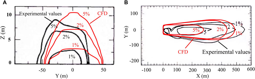
Figure 3. Distribution of methane concentrations across various planes during the Burro nine experiment: (A) the distribution on the Y-Z plane at a distance of 140 m downwind at T = 80 s, and (B) the distribution on the X-Y plane at a height of 1 m, also at T = 80 s.

It specifically depicts the methane concentration over time at a distance of 140 m downwind in Figure 4A, with the observed peak concentration reaching 9.6%. The CFD simulation peaking at 9.62%, resulted in a minimal relative error of 0.2%. While at a distance of 400 m downwind, the observed maximum concentration was 3.96%, compared to the CFD simulation’s maximum value of 3.23%, leading to a relative error of 18.43% (Figure 4B). Sun and Guo (2010) used the DEGADIS model to validate the Burro nine experiment, and the relative errors of the simulation concentrations at downwind distances of 140 m and 400 m were 44.7% and 16.49%, respectively. Sun et al. (2013) simulated the maximum concentrations at different downwind distances of the Burro eight experiment using the Fluent software, with an average relative error of 19.62%. This demonstrates that the CFD model utilized in this study effectively enhanced the precision of concentration prediction, maintaining relative errors within permissible limits. Therefore, the CFD model is considered to accurately capture the trends of the observed methane concentrations, although temporal variations are present. Such variations may arise from the inconsistent evaporation rates of LNG leakage and the dynamics size of the evaporating liquid pool, which, if assumed constant in the model, will introduce validation uncertainties. Figures 4C,D reveal that the simulated heights of the air clouds with varying concentrations at a distance of 400 m downwind slightly exceeded the actual measurements, yet their lateral extents remained broadly consistent. The overall trend alignment and acceptable error margins confirm the CFD simulation’s efficacy for subsequent research.

Figure 4

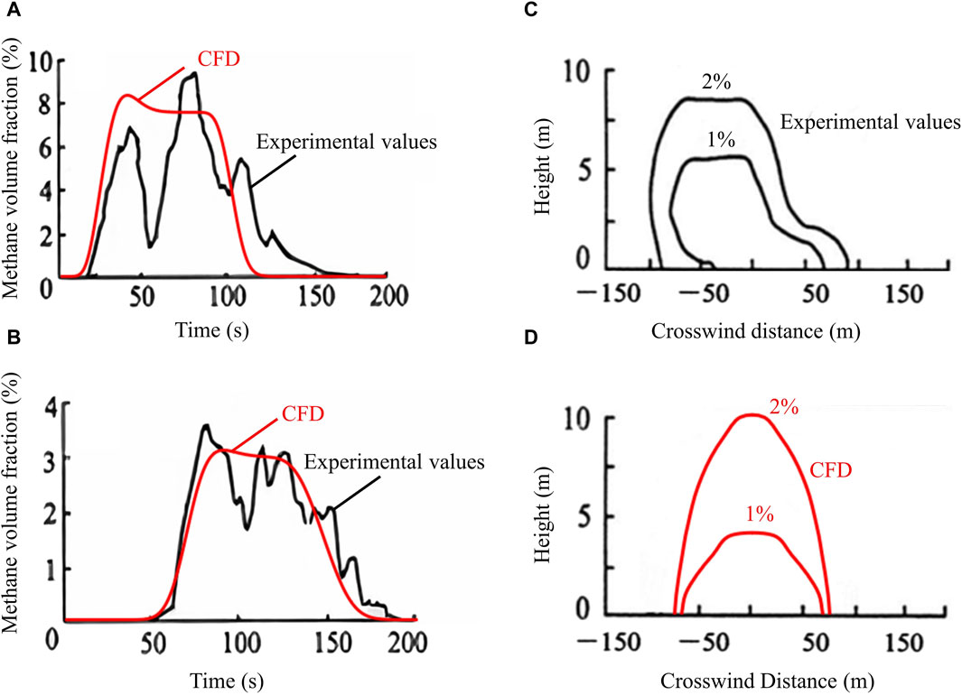
Figure 4. Methane concentration values at different downwind distances for the Burro nine experiment. (A) and (B) are plots of methane concentration values with time at 140 m and 400 m downwind distance, respectively. (C) and (D) are the concentration distributions of experimental and CFD simulated values at T = 120 s and downwind distance of 400 m, respectively.

3 Results and discussion

3.1 Analysis of factors affecting benzene leakage accidents consequences

3.1.1 Dynamic characteristics of liquid pool radius and evaporation rate

Upon the leakage of benzene, its high boiling point resulted in the formation of a liquid pool on the ground. The evaporation of the liquid pool was facilitated by the airflow over the pool surface, with both the radius of the pool and the evaporation rate changing dynamically. Before exploring the impacts of various factors on the diffusion distances of benzene, this study initially analyzed the influences of four factors on the dynamic changes of the radius and evaporation rate of the liquid pool. The results are presented in Figure 5, which displays the dynamic changes of the liquid pool radius and evaporation rate under different wind speeds, temperatures, leakage apertures and atmospheric stabilities, labelled A-L respectively.

Figure 5

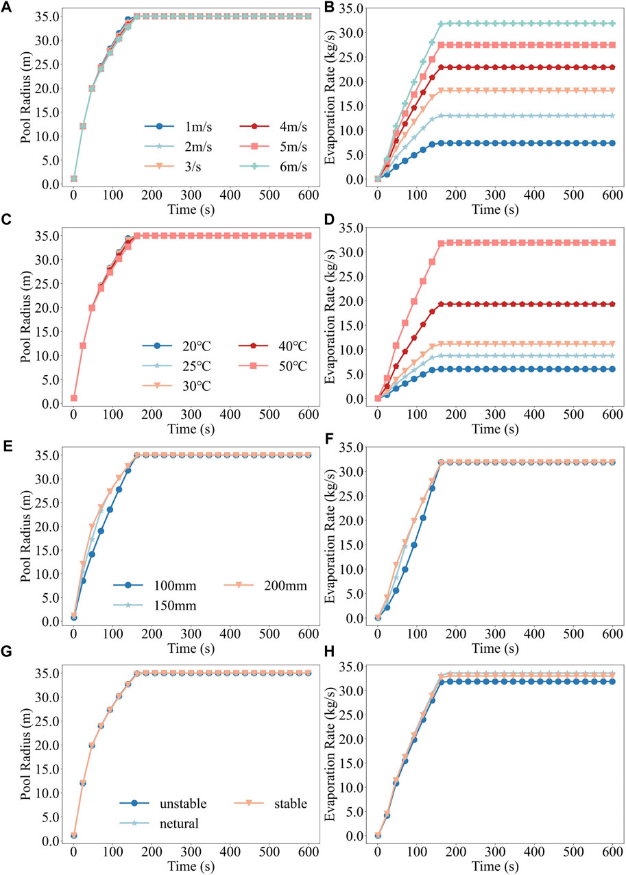
Figure 5. Variation patterns of liquid pool radius and evaporation rate with time under different scenarios, where (A) and (B), (C) and (D), (E) and (F), and (G) and (H) denote the dynamic changes of liquid pool radius and evaporation rate under different wind speeds, temperatures, leakage apertures, and atmospheric stabilities, respectively.

An increase in wind speed from 1 m/s to 6 m/s extended the duration required for the liquid pool to achieve its maximum radius from 145 s to 163 s, currently elevating the evaporation rate from 7.36 kg/s to 31.88 kg/s (Figures 5A,B). This indicates that higher wind speeds not only delay the attainment of the maximum radius of the liquid pool but also substantially enhance the evaporation rate. Such an increase accelerates the volatility and diffusion rate of benzene, thereby enlarging the potential hazardous ranges. Furthermore, a temperature increase from 20°C to 50°C similarly impacted these dynamics, lengthening the time to reach the maximum radius from 144 s to 163 s, while elevating the evaporation rate from 6.03 kg/s to 31.88 kg/s (Figures 5C,D). The rise in temperature not only accelerated the evaporation rate but also slowed down the growth rate of the radius of the liquid pool, prolonging the time to reach its maximum. Variations in the leakage aperture slightly adjusted the time for the liquid pool to achieve its maximum radius from 159 s to 163 s. The evaporation rate attained a consistent peak of 31.88 kg/s at different apertures (Figures 5E,F), indicating a minimal effect of the leakage aperture on the growth of the radius and evaporation rate. Under disparate conditions of atmospheric stability, the radius reached its zenith between 163 s and 165 s, with the lowest evaporation rate under unstable conditions at 31.88 kg/s, and slightly higher under stable and neutral conditions at 33.62 kg/s and 33 kg/s, respectively (Figures 5G,H). Atmospheric stability exerts a minor influence on liquid pool expansion and evaporation rate, as indicated by the coefficients $\alpha$ and $n$ in formula (2). Subsequent research will investigate the effects of these factors on the distribution of concentrations and hazardous distances, providing scientific support for effective risk management and emergency preparedness.

A comprehensive analysis indicated that temperature was the primary factor influencing the growth of the evaporation rate. The impact of wind speed on the radius growth was negligible but significantly enhanced evaporation rate. The impact of leakage aperture and atmospheric stability was insignificant. Related studies (Galeev et al., 2013; Hu et al., 2024) have also emphasized the important role of environmental factors in chemical leakage accidents, in particular the significant effect of wind speed and temperature on the consequences of leakage.

3.1.2 Dynamic characteristics of concentration distribution

To explore the dynamic characteristics of concentration distribution, a specific scenario was chosen for detailed analysis: liquid benzene leakage under stable atmospheric conditions, featuring a 200 mm aperture, a wind speed of 6 m/s and a temperature of 50°C. This study methodically examined the changes in concentration distribution within the hazardous distances for various AEGLs at 150 s, 300 s, 450 s, and 600 s. Figure 6 illustrates the concentration distribution at different times, where A-D, E-H, and I-N correspond to AEGL-1, AEGL-2, and AEGL-3 distances, respectively.

Figure 6

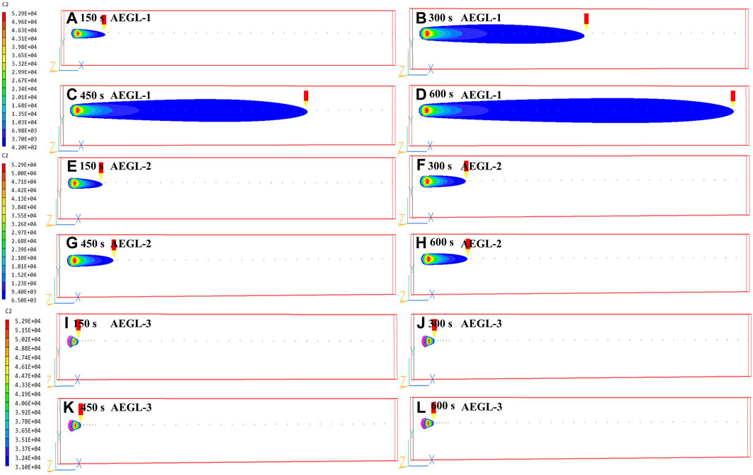
Figure 6. Hazardous ranges corresponding to AEGL-1 (A–D), AEGL-2 (E–H), and AEGL-3 (I–L) at different time (T = 150 s, 300 s, 450 s, 600 s).

Initially, at 150 s, the hazardous range of AEGL-1 was predominantly near the leakage source (Figure 6A). By 600 s, the concentration range had spread to 2780.20 m, revealing a significant downwind stretch while the lateral enlargement of the plume remained comparatively limited (Figure 6D). Compared to AEGL-1, the diffusion rate and the hazardous range of AEGL-2 were markedly reduced. Notably, at 300 and 390 s, the maximum AEGL-2 distance exhibited minimal change, suggesting a plateau in the diffusion speed and expansion range once a certain concentration was reached (Figure 6F). Beyond 300 s, both the downwind distance and plume width remained relatively stable, leading to a more homogeneous distribution of concentration (Figures 6G,H). The diffusion speed and range of AEGL-3 showed an even more pronounced reduction (Figure 6I–L). By 270 s, the hazardous range reached a steady state at 74.27 m, highlighting the restricted diffusion range for high-concentration benzene over a brief period. The lateral expansion of the plume was notably constrained, primarily due to the dominance of wind speed over turbulent mixing, facilitating predominantly downwind diffusion. Consequently, wind speed emerges as a critical determinant in the plume diffusion process, determining the velocity of downwind diffusion (Gong et al., 2023). Meanwhile, initial release conditions, such as leakage rate and temperature, along with local turbulence, play collective roles in shaping the plume width and diffusion uniformity.

3.1.3 Dynamic characteristics of hazardous ranges

In the case of liquid benzene leakage, the hazardous consequences were evaluated using AEGLs distances. The mechanism of the change of AEGLs distances under the four main factors was analyzed by altering the environmental conditions, with the findings illustrated in Figure 7. Notably, the AEGL-1 and AEGL-2 distances increased significantly as temperature rose. The trend for the AEGL-3 distance was only exhibited at higher temperatures. This phenomenon may be attributed to the fact that an increase in temperature elevated the saturated vapor pressure of benzene, thereby expediting the evaporation rate and diffusion process (Yu et al., 2021). Furthermore, for AEGL-3, the concentration value (31,000 mg/m³) represented a high concentration that may be life-threatening following exposure. In this study, it was observed that the distances of AEGL-3 were only present under higher temperatures and were relatively short. This suggested that elevated temperatures may facilitate rapid evaporation of benzene, yet may also facilitate its rapid diffusion and dilution, resulting in rapidly declining concentrations at a distance from the leakage source (Zhou et al., 2024).

Figure 7

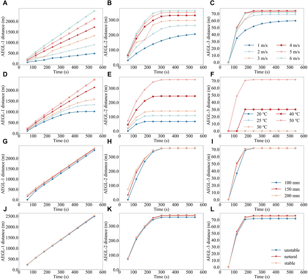
Figure 7. Effects of different factors on the variation of AEGLs distances. (A–C), (D–F), (G–I), and (J–L) indicate the effects of different wind speed, temperature, leakage aperture, and atmospheric stabilities on the AEGL-1, AEGL-2, and AEGL-3 distances, respectively.

Wind speed significantly influenced the diffusion ranges of benzene, with wind speed increasing from 1 m/s to 6 m/s, the AEGL-1, AEGL-2, and AEGL-3 distances exhibiting different growth trends. The increase in diffusion distances was attributed to the turbulent mixing effect at higher wind speeds. However, the extent of this increase was limited, particularly as the AEGL-2 and AEGL-3 distances stabilized more quickly at higher wind speeds. The AEGL-3 distance initially rose with an increase in wind speed until it stabilized approximately 200 s. The maximum distance of 73.93 m was reached at a wind speed of 4 m/s, after which it slightly decreased with further increases in wind speed. Before reaching a steady state in concentration distribution, wind speed primarily served as a mechanism for transporting the cloud over longer distances within the same time frame. Upon reaching a steady state, wind speed facilitated dilution in addition to transportation (Zhou et al., 2021). An increase in wind speed not only enhanced the dilution effect but also accelerated the diffusion speed, thereby narrowing the hazardous range. The impacts of leakage aperture and atmospheric stability on the hazardous distance were minimal. An incremental rise in the AEGL-1 distance was observed with the enlargement of leakage aperture, whereas the AEGL-2 and AEGL-3 distances exhibited negligible changes. Furthermore, the AEGL-1, AEGL-2, and AEGL-3 distances showed no significant variance under different atmospheric stabilities, indicating that over longer periods, atmospheric stability exerted minimal influence on diffusion distances.

3.2 Correlation analysis

Pearson correlation analysis was employed to evaluate the linear relationship between the CFD-simulated methane concentration (C1) and various characteristic variables, including time, leakage aperture, wind speed, temperature, atmospheric stability, and downwind distance. The corresponding results are depicted in Figure 8. Specifically, wind speed and downwind distance were negatively correlated with C1, with correlation coefficients of −0.01 and −0.48, indicating that an increase in wind speed and greater downwind distance resulted in reduced methane concentrations, respectively. Conversely, positive correlations were identified between C1 and variables including time, leakage aperture, temperature, and atmospheric stability, with coefficients of 0.16, 0.01, 0.20, and 0.02, respectively. The strong positive correlation between C1 and time and temperature indicated that higher concentrations were associated with longer leakage time and higher temperature. These findings reveal that there exists a significant but relatively weak correlation between C1 and the characteristic variables, and a nonlinear relationship among the characteristic variables. Given the complexity of the atmospheric diffusion mechanism, which involves nonlinear and dynamic processes affected by various factors, traditional linear models are not the optimal choice. Therefore, it is recommended that a nonlinear model be adopted for a more accurate representation of the complex variable interactions and effects. Furthermore, an analysis of the diffusion mechanism was conducted to robustly support the correlation between the variables, as detailed in the Supplementary Text S2.

Figure 8

Figure 8. Correlation coefficients between characteristic variables and between characteristic variables and the target variable (C1), "×" indicates that the correlation did not pass the significance test at the significance level α = 0.05.

3.3 Feasibility analysis of ML algorithms using CFD standard data

3.3.1 Model performance evaluation

To evaluate the performance of the five ML models on CFD standard data, various evaluation metrics were calculated, as depicted in Figure 9. Figure 9A reveals that R² for the training set among these models varied from 0.962 to 0.999, and IOA varied from 0.990 to 0.999. Notably, R² and IOA of the XGBoost and LightGBM models were both 0.999, indicating nearly-perfect prediction accuracy. In terms of RMSE, the XGBoost model outperformed other models with a score of 181.669 mg/m³, closely followed by the LightGBM model, which scored 204.089 mg/m³. Additionally, these models also exhibited outstanding MAE, with the XGBoost model at 85.742 mg/m³ and the LightGBM model at 108.414 mg/m³, underscoring the exceptional predictive performance of the XGBoost model.

Figure 9

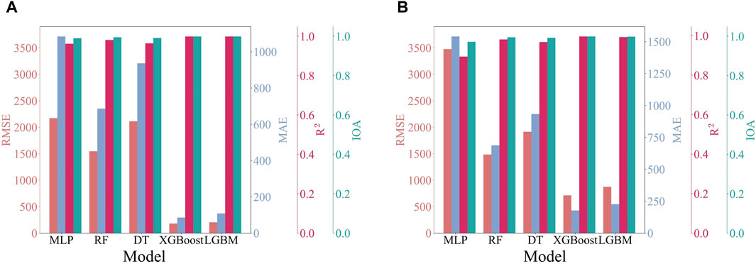
Figure 9. Performance evaluation of predictions based on MLP, RF, DT, XGBoost, and LightGBM models for standard (A) training data and (B) testing data.

On the testing set, both the XGBoost and LightGBM models exhibited strong correlations with R² of 0.996 and 0.993, and IOA of 0.999 and 0.998, respectively (Figure 9B). In contrast, despite the MLP and RF models exhibiting high R² on the training set (0.962 and 0.964, respectively) and acceptable R² on the testing set (0.894 and 0.968), their higher RMSE and MAE suggested a significantly lower prediction accuracy compared to the XGBoost and LightGBM models. The DT model performed well on the training set, with RMSE of 1546.323 mg/m³. Nonetheless, its accuracy decreased on the testing set, with RMSE and MAE of 1483.873 mg/m³ and 686.351 mg/m³, respectively, and slightly lower R² and IOA. This analysis indicates that the MLP and DT models may not be optimal for low-dimensional sample data. However, ensemble models such as the XGBoost and LightGBM models can effectively mitigate the risks of overfitting by integrating multiple simple models, thereby ensuring improved accuracy of concentration prediction.

In the field of environmental science, numerous studies (Li J. et al., 2021; Zang et al., 2021; Xu et al., 2022) have employed a range of ML algorithms to construct prediction models for air pollutant concentrations, with R² primarily falling within the range of 0.68–0.88. In comparison, our models demonstrated a significant improvement in prediction accuracy. Moreover, in the field of risk assessment of accident consequences, related studies (Ni et al., 2020; Wang et al., 2023) have demonstrated the performance of ML models based on CFD simulation data, where R² of the models was higher than 0.90. The ML models constructed on the basis of idealized CFD data in our study, in particular the XGBoost model, not only matched but even outperformed these performance ranges reported by these studies. These results demonstrated the effectiveness of the XGBoost model in terms of prediction accuracy, and illustrated the capacity of the model to process complex and high-dimensional data. The findings suggested the potential applicability of the model in the field of environmental sciences.

3.3.2 Effects of model predictions on concentration accuracy

To further assess the accuracy of various models in predicting concentrations, a validation analysis was performed under a stable atmosphere scenario, characterized by a 200 mm leakage aperture, a wind speed of 6 m/s, and a temperature of 50°C. Concentrations at different distances were compared, with the results presented in Figure 10. This figure demonstrates that the MLP model was unable to accurately predict concentration distributions and trends at both near and distant distances, leading to unsatisfactory outcomes. Conversely, the other models showed improved accuracy in capturing the concentration trends. Notably, from distances of 10 m–500 m, the predictive curves of these models closely aligned with the actual concentration curves, demonstrating high consistency. At a distance of 50 m, all models except the MLP model produced predictions nearly identical to the actual concentrations, with the predictive and actual curves almost overlapping, indicating their robust performance in near-distance prediction. However, the accuracy of these predictions decreased as the distance increased. Beyond 1,000 m, the MLP, DT, and RF models exhibited considerable deviations and were unable to accurately capture the actual concentration distribution and trends, highlighting their limitations in distant-distance concentration prediction. In contrast, the predictive curves of the XGBoost and LightGBM models remained closely aligned with the actual curves, demonstrating their capacity to handle large-scale and complex data effectively. Nevertheless, Figure 10C clearly shows some deviations between the predictive curve of the LightGBM model and the actual concentration curve during abrupt increases. Although the LightGBM model exhibited a slightly stable trend aligning with the actual values in high concentration ranges (Figures 10A,B), the XGBoost model adapted more quickly to near-actual values in rapidly changing concentrations (Figures 10E,H). This indicated that the XGBoost model may provide more timely decision support in dynamic prediction scenarios. Considering their performance with respect to prediction latency and accuracy in high concentration intervals, the XGBoost model outperformed the LightGBM model, corroborating the findings discussed in Section 3.3.1. These results provide a scientific framework for model selection in particular scenarios.

Figure 10

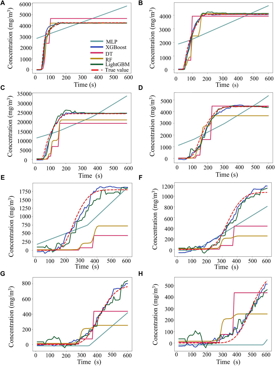
Figure 10. Comparison of model validation for concentration at different downwind distances: (A), (B), (C), (D), (E), (F), (G), and (H) correspond to the predicted versus the true values of the different models at downwind distances of 10, 50, 100, 500, 1,000, 1,500, 2000, and 2,500 m, respectively.

3.4 Evaluation of ML algorithms based on noisy data

3.4.1 Model performance evaluation

In order to more closely match real-world measured data and to evaluate the generalizability of the model, noise is often introduced into the standard data to mimic real-world variations (Li X. et al., 2021). Therefore, Gaussian noise was incorporated into the CFD standard data and the mean and variance of the Gaussian noise were adjusted to generate datasets with different noise levels. The performance of each model on the training and testing data was evaluated with a noise scale of 0.5, and the results of this evaluation are depicted in Figure 11.

Figure 11

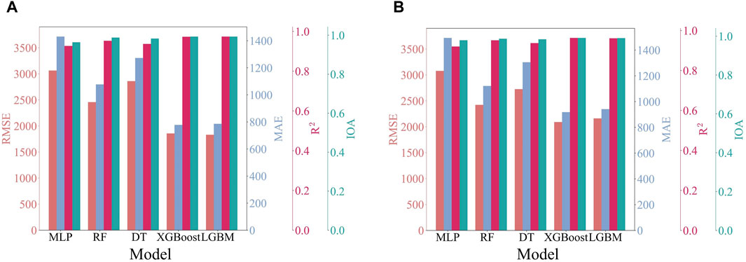
Figure 11. Performance evaluation of predictions based on MLP, RF, DT, XGBoost, and LightGBM models for noisy (A) training data and (B) testing data.

Figure 11 shows that the MLP model achieved RMSE and MAE of 3062.884 mg/m³ and 1430.555 mg/m³ on the training set, and 3078.269 mg/m³ and 1494.641 mg/m³ on the testing set, respectively. Although the DT and RF models performed slightly better in terms of RMSE and MAE, they still exhibited significant sensitivity to the presence of noise. In comparison, both the XGBoost and LightGBM models demonstrated exceptional performance across all evaluation metrics, with the lowest RMSE and MAE. RMSE for the XGBoost and LightGBM models on the training data were 1856.175 mg/m³ and 1831.244 mg/m³, respectively, while MAE were 778.301 mg/m³ and 785.941 mg/m³, respectively. R² was 0.973 for the XGBoost model and 0.974 for the LightGBM model, with both models achieving IOA of 0.993. The difference in performance between the two models was minimal, with the LightGBM model slightly outperforming in terms of predictive accuracy. On the testing data, RMSE for the XGBoost and LightGBM models were 2091.083 mg/m³ and 2162.072 mg/m³, with MAE were 918.705 mg/m³ and 41.887 mg/m³, respectively. R² was 0.963 and 0.961, and IOA was 0.991 and 0.990, respectively. Here, the performance of the XGBoost model was more pronounced. Overall, both models demonstrated high robustness in processing and predicting noisy data, which is vital for the effective operation of ML algorithms in diverse real-world situations. Nevertheless, the XGBoost model displayed an advantage in predictive accuracy and stability.

Previous studies (Ni et al., 2020; Wang et al., 2023) have typically constructed ML prediction models based on idealized data from CFD simulations. However, in real-world environments, real data frequently contain noise due to monitoring equipment failures and measurement errors. This study sought to assess the reliability of the predictive performance of ML models based on noisy data by adding noise to the data to reflect the real-world situation, and enhance the robustness and generalization of the models. The results demonstrated that the XGBoost model exhibited excellent predictive performance despite the presence of noise.

3.4.2 Effects of model predictions on concentration accuracy

A comparative analysis of concentration predictions at various distances from the source was performed using noisy data, with the results illustrated in Figure 12. The analysis clearly indicated that as the downwind distance increases, the difference between the predictions of the models and the noise values also increased, indicating a higher level of uncertainty in the prediction. At near distances, the’ predictions of all models were closer to the actual values. However, at distant distances, the prediction curves become more volatile, with the MLP model’s predictions deviating significantly from the true values. The MLP model was ineffective in predicting noisy data. The DT and RF models, while providing predictions closer to the true values, did not accurately reflect the overall trends. Conversely, the XGBoost and LightGBM models demonstrated exceptional predictive performance, accurately capturing changes in concentration trends at both near and distant distances. This evidence reinforces the notion that ensemble models, especially the XGBoost and LightGBM models, exhibit strong generalization capabilities and robustness in both standard and noisy data, excelling in predicting concentration distributions and trends effectively. Overall, the inherent features of ensemble models, such as model averaging, robustness, and overfitting prevention, contribute to their effectiveness in making reliable predictions within noisy environments (Cong et al., 2023). These attributes render ensemble models indispensable tools for addressing the complexity and uncertainty inherent in real-world data.

Figure 12

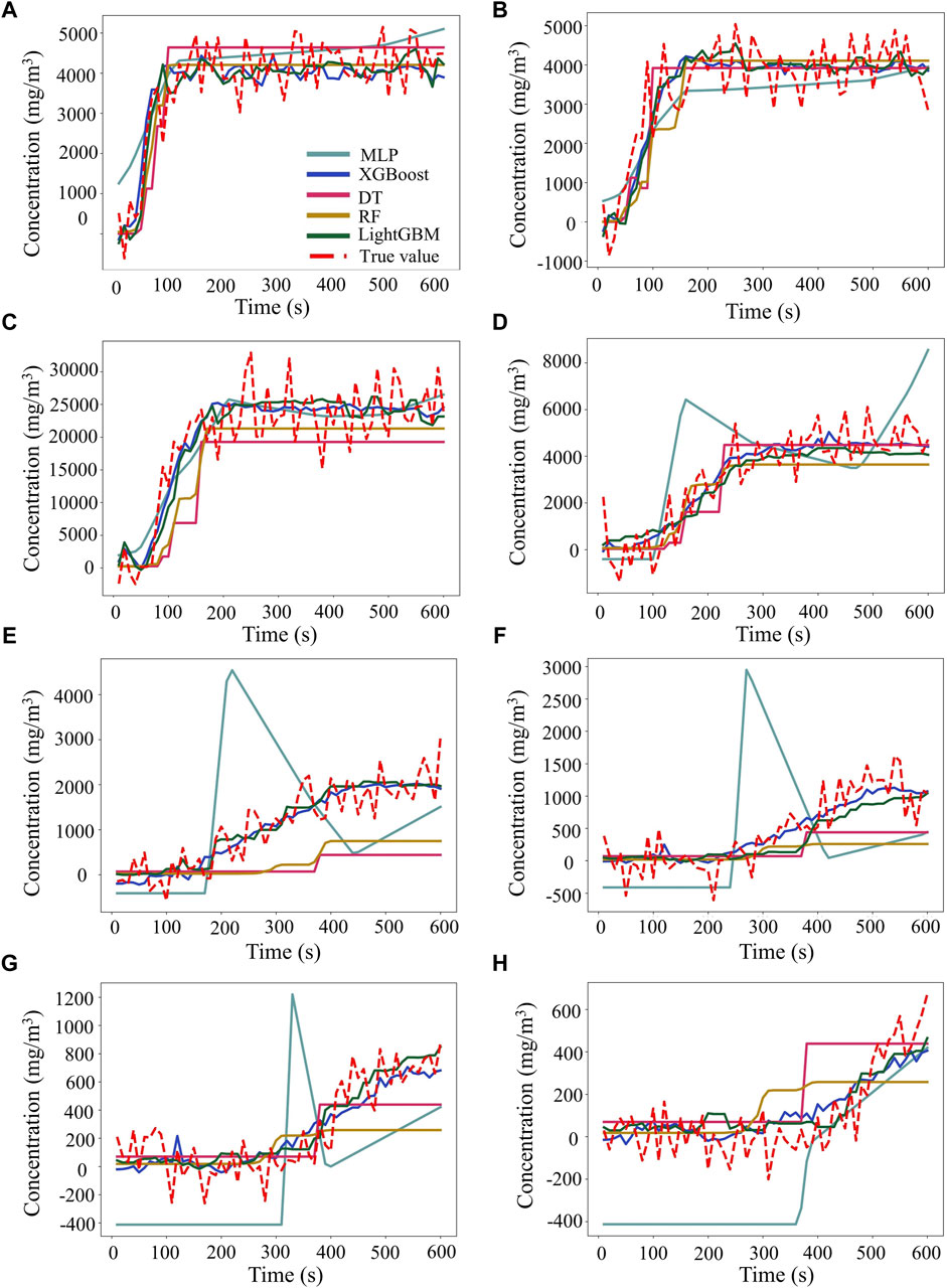
Figure 12. The comparison of model validation for concentrations at different downwind distances: (A), (B), (C), (D), (E), (F), (G), (H) correspond to the predicted values versus the true values of the different models at downwind distances of 10, 50, 100, 500, 1,000, 1,500, 2000, 2,500 m, respectively.

3.4.3 Analysis of predictive application using the XGBoost model

In emergency rescue operations, accurately predicting the temporal distribution of hazardous chemical concentration over time and the corresponding hazardous distances for concentration limits is essential for devising the effective emergency response strategies. This study evaluated the efficiency of the XGBoost model in predicting the diffusion of liquid benzene leakage following a leakage from a tank with a 200 mm aperture under conditions of a 6 m/s wind speed, a 50°C temperature, and stable atmospheric conditions. The aim is to replicate an industrial scenario with specific environmental parameters. The comparison between CFD simulation results and hazardous distance predictions from the XGBoost model, as presented in Figure 13, underscores the exceptional ability of the model in accurately predicting benzene concentration levels and determining hazardous distances. Specifically, the XGBoost model demonstrates the capacity to accurately predict concentrations at different distances, whether near the leakage source or at distant distances. Notably, Figure 13A confirms the accuracy of the model in matching saturation concentrations, whereas Figures 13B,C indicate a minor temporal delay in the model’s predictions compared to the actual values, suggesting a negligible hysteresis effect without compromising overall accuracy. Moreover, the model demonstrated exceptional alignment with real-world distances for AEGL-1, AEGL-2, and AEGL-3, with minimal relative errors. Specifically, it predicted distances of 2705.1 m, 378.4 m, and 74.44 m against the true distances of 2780.2 m, 368.9 m, and 74.27 m, achieving relative errors of 2.70%, 2.58%, and 0.23%, respectively. Compared to the CFD model, the enhanced efficacy and speed exhibited by the XGBoost model indicate that ML algorithms may significantly improve the real-time emergency response capabilities, potentially reducing the risks these accidents pose to humans and the environment. In addition, the XGBoost model exhibited a markedly superior predictive efficiency compared to the CFD model, resulting in significant savings in computational costs. The model took only 0.218 s to output the prediction results when running on a computer with an AMD Ralon R7 6800H CPU and 32G of RAM, while the CFD model took about 3 h to complete a simulation on a computer with an 11th Gen Intel^® Core (TM) i5-11400H CPU and 8G of RAM for this leakage scenario. It should be noted that the simulation time may vary depending on the specific leakage scenario under consideration. Obviously, using ML algorithms can significantly improve the prediction efficiency and meet the current demand for dynamic, accurate and fast predictions in smart parks.

Figure 13

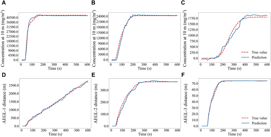
Figure 13. Comparison of predicted and true values of concentrations at various downwind distances and hazardous distances based on the XGBoost model, (A), (B), and (C) correspond to downwind distances of 10, 100, and 1,000 m, respectively. (D), (E), and (F) correspond to AEGL-1, AEGL-2, and AEGL-3 distances, respectively.

The precise prediction of hazardous distances is crucial for assessing the consequences of leakage accidents and for immediate emergency response measures. The investigation of XGBoost models that not only provide accurate predictions but also maintain prediction efficiency has enabled the fast provision of prediction ranges for emergency response. It is recommended that further development and integration of ML techniques for the prediction and management of hazardous situation be a priority in industrial safety and environmental protection strategies.

4 Conclusion

This study examined the consequences of chemical leakage accidents by simulating Burro series experiments using the CFD (PHOENICS version 6.0) model. The simulations were benchmarked against Burro nine data, revealing a strong correlation between the simulated and observed concentrations within acceptable discrepancies, thereby affirming the efficacy of the CFD model in simulating the heavy gas leakage diffusion. Using liquid benzene as an example, a CFD-based dynamic model was developed to analyze the consequences of heavy gas leakage diffusion, examining the impacts of wind speed, temperature, leakage aperture, and atmospheric stability. The analysis underscored the pivotal roles of wind speed and temperature in influencing the distribution patterns of liquid benzene concentrations and AEGLs distances over extended periods. In contrast, leakage aperture and atmospheric stability minimally affected the hazardous distances. Furthermore, five ML models were developed using CFD standard and noisy data. The performance assessment revealed that the XGBoost model surpassed the other models for concentration simulation, demonstrating resilience to noise interference. Consequently, a fast prediction model for the dynamic diffusion of heavy gas leakage based on the XGBoost model was established. This model’s precision was confirmed by comparing actual and predicted concentrations at various downwind distances and hazardous distances. The relative errors between the actual values and predictions of AEGL-1, AEGL-2, and AEGL-3 distances were 2.70%, 2.58%, and 0.23%, respectively. More importantly, the XGBoost model demonstrated exceptional efficiency, generating predictions in only 0.218 s, significantly faster than the CFD model. This efficiency, coupled with reduced computational demands, positioned ML algorithms as vital tools for dynamic and precise emergency response planning in smart parks, highlighting their potential in enhancing future response strategies.

However, it is essential to acknowledge the uncertainties and limitations inherent in our study. The reliance on data-driven models, particularly the opaque nature of ML algorithms, introduces uncertainties in understanding dynamic mechanisms. Additionally, despite utilizing CFD outputs augmented with Gaussian noise, it still differs from actual leakage scenarios. Furthermore, the applicability of our model is confined to open-space leakage incidents, omitting the influence of complex terrains and various underlying surface types on predictive accuracy. The efficacy of the XGBoost model in handling complex terrains or enclosed spaces necessitates further investigation. This opens up new avenues for our future research in this field. Future directions include incorporating real observational data, employing sophisticated data assimilation techniques for improved precision, and expanding the model to encompass a wider array of factors and scenarios.

Data availability statement

The original contributions presented in the study are included in the article/Supplementary Material, further inquiries can be directed to the corresponding author.

Author contributions

CF: Writing–original draft, Writing–review and editing. HG: Writing–review and editing. YZ: Writing–review and editing. WM: Writing–review and editing. QY: Writing–review and editing.

Funding

The author(s) declare that no financial support was received for the research, authorship, and/or publication of this article. The author(s) declare that no financial support was received for the research, authorship, and/or publication of this article.

Acknowledgments

We really appreciate the editors and reviewers for their meaningful comments for improving our manuscript.

Conflict of interest

The authors declare that the research was conducted in the absence of any commercial or financial relationships that could be construed as a potential conflict of interest.

Publisher’s note

All claims expressed in this article are solely those of the authors and do not necessarily represent those of their affiliated organizations, or those of the publisher, the editors and the reviewers. Any product that may be evaluated in this article, or claim that may be made by its manufacturer, is not guaranteed or endorsed by the publisher.

Supplementary material

The Supplementary Material for this article can be found online at: https://www.frontiersin.org/articles/10.3389/fenvs.2024.1409072/full#supplementary-material

References

Ahmed, S., Adnan, M., Janssens, D., and Wets, G. (2020). A Route to School Informational Intervention for Air Pollution Exposure Reduction. Sustain. Cities Soc. 53, 101965. doi:10.1016/j.scs.2019.101965

CrossRef Full Text | Google Scholar

Arsic, M., Mihajlović, I., Nikolić, D., Živković, Ž., and Panić, M. (2020). Prediction of Ozone Concentration in Ambient Air Using multilinear Regression and the Artificial Neural Networks Methods. Ozone Sci. Eng. 42, 79–88. doi:10.1080/01919512.2019.1598844

CrossRef Full Text | Google Scholar

Barjoee, S. S., Elmi, M. R., Varaoon, V. T., Keykhosravi, S. S., and Karimi, F. (2022). Hazards of Toluene Storage Tanks in a Petrochemical Plant: Modeling Effects, Consequence Analysis, and Comparison of Two Modeling Programs. Environ. Sci. Pollut. Res. Int. 29, 4587–4615. doi:10.1007/s11356-021-15864-5

PubMed Abstract | CrossRef Full Text | Google Scholar

Breiman, L. (2001). Random Forests. Mach. Learn. 45, 5–32. doi:10.1023/a:1010933404324

CrossRef Full Text | Google Scholar

Bruha, I. (2000). From Machine Learning to Knowledge Discovery: Survey of Preprocessing and Postprocessing. Intell. Data Anal. 4, 363–374. doi:10.3233/ida-2000-43-413

CrossRef Full Text | Google Scholar

Bu, F. X., Liu, Y., Chen, S., Wu, J., Guan, B., Zhang, N., et al. (2022). Real scenario analysis of buried natural gas pipeline leakage based on soil-atmosphere coupling. Int. J. Press. Vessels Pip. 199, 104713. doi:10.1016/j.ijpvp.2022.104713

CrossRef Full Text | Google Scholar

Chai, H., Jin, X., Xu, C., and Xia, C. (2023). Review of Machine Learning-based 5G for Industrial Internet of Things. Inf. Control 52, 257–276. doi:10.13976/j.cnki.xk.2023.2574

CrossRef Full Text | Google Scholar

Chen, J., Mu, F., Zhang, Y., Tian, T., and Wang, J. (2022). Comparative Analysis of Hourly PM_(2.5) Prediction Based on Multiple Machine Learning Models. J Nanjing For. Univ. 46, 152–160. doi:10.12302/j.issn.1000-2006.202106023

CrossRef Full Text | Google Scholar

Chen, T., and Guestrin, C. (2016). “XGBoost: A Scalable Tree Boosting System,” in Proceedings of the 22nd Acm Sigkdd International Conference on Knowledge Discovery and Data Mining. San Francisco, California, USA: Association for Computing Machinery, 785–794.

Google Scholar

Cheng, C., Xia, T., and Pang, Q. (2022). Simulation Study on Consequences of Ethylene Oxide Storage Tank Leakage Accidents in Summer and Winter. Saf. Environ. Eng. 29, 156–162. doi:10.13578/j.cnki.issn.1671-1556.20211463

CrossRef Full Text | Google Scholar

Cong, J., Cheng, P., and Zhao, Z. (2023). The Integrated Forecasting Model of Stock Index Based on CEEMD-CNN-LSTM. Syst. Eng. 41, 104–116.

Google Scholar

Ehteram, M., Panahi, F., Ahmed, A. N., Huang, Y. F., Kumar, P., and Elshafie, A. (2022). Predicting Evaporation with Optimized Artificial Neural Network Using Multi-Objective Salp Swarm Algorithm. Environ. Sci. Pollut. Res. Int. 29, 10675–10701. doi:10.1007/s11356-021-16301-3

PubMed Abstract | CrossRef Full Text | Google Scholar

Fang, X., Duan, H., Hu, M., and Cai, J. (2019). The Seasonal Differential Effects of Meteorological Parameters on Atmospheric Pollutants and the Prediction Model Comparison: A Case Study of Shenzhen. Environ. Pollut. Control 41, 541–546. doi:10.15985/j.cnki.1001-3865.2019.05.009

CrossRef Full Text | Google Scholar

Fu, L. I. (2008). Bernoulli’s Equation for Compressible Flow. Coll. Phys. 27, 15. doi:10.3969/j.issn.1000-0712.2008.08.005

CrossRef Full Text | Google Scholar

Fu, W.-X., Huang, L., Ding, J. H., Qin, M. M., Yu, X. N., Xie, F. J., et al. (2023). Elucidating the Impacts of Meteorology and Emission Changes on Concentrations of Major Air Pollutants in Major Cities in the Yangtze River Delta Region Using a Machine Learning De-weather Method. Environ. Sci. 44, 5879–5888. doi:10.13227/j.hjkx.202301119

CrossRef Full Text | Google Scholar

Galeev, A. D., Salin, A., and Ponikarov, S. (2013). Consequence Analysis of Aqueous Ammonia Spill Using Computational Fluid Dynamics. J. Loss Prev. Process Ind. 26, 628–638. doi:10.1016/j.jlp.2012.12.006

CrossRef Full Text | Google Scholar

Gao, M., Zhang, Y., Zhang, R., Huang, Z., Huang, L., Li, F., et al. (2020). Air Quality Prediction Approach Based on Integrating Forecasting Dataset. J. Shandong Univ. Eng. Sci. 50, 91–99. doi:10.6040/j.issn.1672-3961.0.2019.404

CrossRef Full Text | Google Scholar

Gong, H. X., Wang, Y. Y., Wang, G. Y., Gao, Y. Q., Li, G., and Kuang, Z. X. (2023). Quantifying the spatial representativeness of carbon flux footprints of a grassland ecosystem in the semi-arid region. J. Geophy. Res. Atmosph. 128. doi:10.1029/2022JD038269

CrossRef Full Text | Google Scholar

Hu, X. M., Su, M., Chen, X., Wang, Y., Yu, S., and Zhao, Y. (2024). Numerical Study on Leakage Dispersion Pattern and Hazardous Area of Ammonia Storage Tanks. Energy Technol. 12, 2301067. doi:10.1002/ente.202301067

CrossRef Full Text | Google Scholar

Jiao, Z. R., Ji, C., Sun, Y., Hong, Y., and Wang, Q. (2021). Deep Learning Based Quantitative Property-Consequence Relationship (QPCR) Models For Toxic Dispersion Prediction. Process Saf. Environ. Prot. 152, 352–360. doi:10.1016/j.psep.2021.06.019

CrossRef Full Text | Google Scholar

Kang, D., Liu, L., and Ji, H. (2017). Construction of Intelligent Emergency Rescue Platform for Chemical Industry Park. Chem. Ind. Eng. Prog. 36, 1544–1549. doi:10.16085/j.issn.1000-6613.2017.04.051

CrossRef Full Text | Google Scholar

Kang, J., Huang, L., Zhang, C., Zeng, Z., and Yao, S. (2020). Hourly PM2.5 Prediction and Its Comparative Analysis Under Multi-Machine Learning Model. China Environ. Sci. 40, 1895–1905. doi:10.3969/j.issn.1000-6923.2020.05.005

CrossRef Full Text | Google Scholar

Koopman, R. P., Cederwall, R., Ermak, D., Goldwire, H., Hogan, W., McClure, J., et al. (1982). Analysis of Burro Series 40-m3 LNG Spill Experiments. J. Hazard. Mater. 6, 43–83. doi:10.1016/0304-3894(82)80034-4

CrossRef Full Text | Google Scholar

Li, H., Shi, Y., Xiong, M., and Li, C. (2019). Study on Impact of Leakage of Toxic and Hazardous Gases on Habitability of Main Control Room Based on ALOHA. Nucl. Power Eng. 40, 126–130. doi:10.13832/j.jnpe.2019.01.0126

CrossRef Full Text | Google Scholar

Li, J., Wei, P., Dai, X., Zhao, S., Zhang, B., Lu, L., et al. (2021a). Optimization of Numerical Simulation in Xi’an Based on Machine Learning Methods. Res. Environ. Sci. 34, 872–881.

Google Scholar

Li, P., and Tian, J. (2011). Characteristics of Surface Layer Wind Speed Profiles over Different Underlying Surfaces. Resour. Sci. 33, 2005–2010.

Google Scholar

Li, X., Jiang, Z., Shan, C., Liu, C., and He, C. (2017). Intelligent Approach for Analyzing Surveillance Videos in Urban Emergency Management. Comput. Eng. Appl. 53, 154–160. doi:10.3778/j.issn.1002-8331.1606-0382

CrossRef Full Text | Google Scholar

Li, X., Li, T., and Ma, J. (2021b). Soft Prediction of Coal-mine Gas Concentration through the Mixture of Gaussian Processes Under the Noisy Input Prediction Strategy. J. Signal. P 37, 2031–2040. doi:10.16798/j.issn.1003-0530.2021.11.003

CrossRef Full Text | Google Scholar

Li, Z., Liang, X., Jin, Y., Zhang, H., and Ou, Y. (2021c). A Comparative Study on Edictive Effect of PM2.5 in Beijing Based on Tree Models. Environ. Eng. 39, 106–113. doi:10.13205/j.hjgc.202106016

CrossRef Full Text | Google Scholar

Liu, J., and Li, L. (2013). Substances of Very High Concern: Challenge to Risk Management System, Capability and Fundamental Research of Chemicals in China. Chin. Sci. Bull. 58, 2643–2650. doi:10.1360/972013-231

CrossRef Full Text | Google Scholar

Liu, X., Wang, Z., Ouyang, J., and Yang, T. (2023). A Quantitative Noise Method to Evaluate Machine Learning Algorithm on Multi-Fidelity Data. J. Chin. Ceram. Soc. 51, 405–410. doi:10.14062/j.issn.0454-5648.20220811

CrossRef Full Text | Google Scholar

Liu, Y. C., and Wang, J. (2022). Numerical Simulation Analysis of Fire Hazard from Leakage and Diffusion of Vinyl Chloride in Different Atmospheric Environments. Fire-Basel 5, 36. doi:10.3390/fire5020036

CrossRef Full Text | Google Scholar

Lu, H., et al. (2020). Adjusting PM_(2.5) Prediction of the Numerical Air Quality Forecast Model Based on Machine Learning Methods in Chengyu Region. Acta Sci. Circumstantiae 40, 4419–4431. doi:10.13671/j.hjkxxb.2020.0317

CrossRef Full Text | Google Scholar

Ma, Z. W., Dey, S., Christopher, S., Liu, R., Bi, J., Balyan, P., et al. (2022). A Review of Statistical Methods Used for Developing Large-Scale and Long-Term PM2.5 Models from Satellite Data. Remote Sens. Environ. 269, 112827. doi:10.1016/j.rse.2021.112827

CrossRef Full Text | Google Scholar

Ni, J., Yang, H., Yao, J., Li, Z., and Qin, P. (2020). Toxic Gas Dispersion Prediction For Point Source Emission Using Deep Learning Method. Hum. Ecol. Risk Assess. 26, 557–570. doi:10.1080/10807039.2018.1526632

CrossRef Full Text | Google Scholar

Nielsen, F., Olsen, E., and Fredenslund, A. (1995). Prediction of Isothermal Evaporation Rates of Pure Volatile Organic-Compounds in Occupational Environments-A Theoretical Approach Based on Laminar Bouundary-Layer Theory. Ann. Occup. Hyg. 39, 497–511. doi:10.1016/0003-4878(95)00032-a

CrossRef Full Text | Google Scholar

Pan, X., and Jiang, J. (2004). Real-Time Environment Risk Analysis for Accident Release of Hazardous Materials Around Tank Area. Acta Sci. Circumstantiae 24, 539–544. doi:10.3321/j.issn:0253-2468.2004.03.030

CrossRef Full Text | Google Scholar

Peng, H., Zhou, Y., Hu, X., Zhang, L., Peng, Y., and Cai, X. (2023). A PM (2.5) Prediction Model Based on Deep Learning and Random Forest. Natl. Remote Sens. Bull. 27, 430–440. doi:10.11834/jrs.20210504

CrossRef Full Text | Google Scholar

Qiu, S. H., Chen, B., Wang, R., Zhu, Z., Wang, Y., and Qiu, X. (2017). Estimating Contaminant Source in Chemical Industry Park Using UAV-Based Monitoring Platform, Artificial Neural Network and Atmospheric Dispersion Simulation. Rsc Adv. 7, 39726–39738. doi:10.1039/c7ra05637k

CrossRef Full Text | Google Scholar

Qiu, S. H., Chen, B., Wang, R., Zhu, Z., Wang, Y., and Qiu, X. (2018). Atmospheric Dispersion Prediction and Source Estimation of Hazardous Gas Using Artificial Neural Network, Particle Swarm Optimization and Expectation Maximization. Atmos. Environ. 178, 158–163. doi:10.1016/j.atmosenv.2018.01.056

CrossRef Full Text | Google Scholar

Shaik, N. B., Benjapolakul, W., Pedapati, S. R., Bingi, K., Thien Le, N., Asdornwised, W., et al. (2022). Recurrent Neural Network-Based Model for Estimating the Life Condition of a Dry Gas Pipeline. Process Saf. Environ. Prot. 164, 639–650. doi:10.1016/j.psep.2022.06.047

CrossRef Full Text | Google Scholar

Shaik, N. B., Pedapati, S. R., Othman, A. R., and Dzubir, F. A. B. A. (2023). “A Case Study to Predict Structural Health of a Gasoline Pipeline Using ANN and GPR Approaches,” in ICPER 2020. Singapore: Springer Nature Singapore, 611–624.

CrossRef Full Text | Google Scholar

Shaik, N. B., Jongkittinarukorn, K., Benjapolakul, W., and Bingi, K. (2024). A Novel Neural Network-Based Framework to Estimate Oil and Gas Pipelines Life with Missing Input Parameters. Sci. Rep. 14, 4511. doi:10.1038/s41598-024-54964-3

PubMed Abstract | CrossRef Full Text | Google Scholar

So, W., Koo, J., Shin, D., and Yoon, E. S. (2010). The Estimation of Hazardous Gas Release Rate Using Optical Sensor and Neural Network. 20th Eur. Symposium Comput. Aided Process Eng. 28, 199–204. doi:10.1016/s1570-7946(10)28034-3

CrossRef Full Text | Google Scholar

Sun, B., and Guo, K. (2010). Safety Exclusive Distance of LNG Dense Gas Dispersion and Its Influencing Factors. Nat. Gas. Ind. 30, 110–113. doi:10.3787/j.issn.1000-0976.2010.07.029

CrossRef Full Text | Google Scholar

Sun, B., Utikar, R. P., Pareek, V. K., and Guo, K. (2013). Computational Fluid Dynamics Analysis of Liquefied Natural Gas Dispersion for Risk Assessment Strategies. J. Loss Prev. Process Ind. 26, 117–128. doi:10.1016/j.jlp.2012.10.002

CrossRef Full Text | Google Scholar

Terzioglu, L., and Iskender, H. (2021). Modeling the Consequences of Gas Leakage and Explosion Fire in Liquefied Petroleum Gas Storage Tank in Istanbul Technical University, Maslak Campus. Process Saf. Prog. 40, 319–326. doi:10.1002/prs.12263

CrossRef Full Text | Google Scholar

Wang, B., Chen, B., and Zhao, J. (2015). The Real-Time Estimation of Hazardous Gas Dispersion by the Integration of Gas Detectors, Neural Network and Gas Dispersion Models. J. Hazard. Mater. 300, 433–442. doi:10.1016/j.jhazmat.2015.07.028

PubMed Abstract | CrossRef Full Text | Google Scholar

Wang, B., Qian, F., and Zhong, W. (2019). Wind Field Reconstruction for the Dispersion Modeling of Accidental Chemical Spills on Complex Geometry. Chin. J. Chem. Eng. 27, 2712–2724. doi:10.1016/j.cjche.2019.02.029

CrossRef Full Text | Google Scholar

Wang, H., Yang, W., Huang, W., and Li, H. (2023). Research On XGBoost Prediction Method for Emergency Rescue Area of Liquid Ammonia Leakage. J. Saf. Environ. 23, 1482–1489. doi:10.13637/j.issn.1009-6094.2022.2546

CrossRef Full Text | Google Scholar

Wang, L., Kang, H., and Xu, K. (2017). Intelligent Park Power System Management Platform Based on Big Data. Chin. J. Power Sources 41, 1637–1639. doi:10.3969/j.issn.1002-087X.2017.11.041

CrossRef Full Text | Google Scholar

Wang, X., Yu, X., and Wang, T. (2021). Air Pollution Impact Prediction of Chemical Industry Park Based on Ensemble Learning Strategy. Oper. Res. Manage. Sci. 30, 127–134. doi:10.12005/orms.2021.0360

CrossRef Full Text | Google Scholar

Wei, J., Li, Z., Pinker, R. T., Wang, J., Sun, L., Xue, W., et al. (2021). Himawari-8-Derived Diurnal Variations in Ground-Level PM2.5 Pollution Across China Using The Fast Space-Time Light Gradient Boosting Machine (LightGBM). Atmos. Chem. Phys. 21, 7863–7880. doi:10.5194/acp-21-7863-2021

CrossRef Full Text | Google Scholar

Wu, J., and Zhao, P. (2013). A Missing Values Filling Algorithm Based on Random Forest for Non-Linear Noisy Datasets. Comput. Appl. Softw. 30, 51–53. doi:10.3969/j.issn.1000-386x.2013.07.015

CrossRef Full Text | Google Scholar

Wu, L. W., Qiao, L., Fan, J., Wen, J., Zhang, Y., and Jar, B. (2024). Investigation on Natural Gas Leakage and Diffusion Characteristics Based on CFD. Gas. Sci. Eng. 123, 205238. doi:10.1016/j.jgsce.2024.205238

CrossRef Full Text | Google Scholar

Xu, F., Li, J., Chu, X., and Man, Y. (2022). Simulation of Daily PM_(2.5) Based on MODIS Data and Multi-Machine Learning Method. China Environ. Sci. 42, 2523–2529. doi:10.3969/j.issn.1000-6923.2022.06.005

CrossRef Full Text | Google Scholar

Yu, C., Liu, R., Luo, T., Zhang, J., Qu, S., Bi, M., et al. (2018). Numerical Simulation of Heavy Gas Dispersion. Cryogenics, 45–51. doi:10.3969/j.issn.1000-6516.2018.03.010

CrossRef Full Text | Google Scholar

Yu, D., Li, J., and Luo, Y. (2019). Application of Random Forests and Decision Trees in the Prognosis of Upper Gastrointestinal Bleeding in Patients with Liver Cirrhosis. Chin. J. Health Stat. 36, 162–166.

Google Scholar

Yu, H., Pu, L., Gao, Q., Sun, R., and Dai, M. (2021). Numerical Study on the Influence of Environmental Factors on the Diffusion Process of Liquid Oxygen Leakage. J. Xi’an Jiaot. Univ. 55, 119–129. doi:10.7652/xjtuxb202108015

CrossRef Full Text | Google Scholar

Zang, Z., Guo, Y., Jiang, Y., Zuo, C., Shi, W., et al. (2021). Tree-Based Ensemble Deep Learning Model for Spatiotemporal Surface Ozone (O3) Prediction and Interpretation. Int. J. Appl. Earth Obs. 103, 102516. doi:10.1016/j.jag.2021.102516

CrossRef Full Text | Google Scholar

Zhang, J., Yu, A. N., and Lijun, W. E. I. (2007). Review on Atmospheric Dispersion Response to Chemical Models for Emergency Accidents. China Saf. Sci. J. 17, 12–17. doi:10.3969/j.issn.1003-3033.2007.06.002

CrossRef Full Text | Google Scholar

Zhang, L., Lin, J., Qiu, R., Hu, X., Zhang, H., Chen, Q., et al. (2018). Trend Analysis and Forecast of PM2.5 in Fuzhou, China Using the ARIMA Model. Ecol. Indic. 95, 702–710. doi:10.1016/j.ecolind.2018.08.032

CrossRef Full Text | Google Scholar

Zhang, X. B., Li, J., Zhu, J., and Qiu, L. (2015). Computational Fluid Dynamics Study on Liquefied Natural Gas Dispersion with Phase Change of Water. Int. J. Heat. Mass Tran. 91, 347–354. doi:10.1016/j.ijheatmasstransfer.2015.07.117

CrossRef Full Text | Google Scholar

Zhao, M., and Chen, Q. (2014). Study on Method of Regional Risk Assessment for Urban Major Hazard. J. Saf. Sci. Technol. 10, 158–164. doi:10.11731/j.issn.1673-193x.2014.09.027

CrossRef Full Text | Google Scholar

Zhou, N., Zhang, Q., Li, X., Chen, L., Liu, X., Lu, X., et al. (2021). Numerical Simulation of the Effect of Wind Speed on LNG Leakage and the Diffusion Process. J. Saf. Environ. 21, 285–294. doi:10.13637/j.issn.1009-6094.2019.0909

CrossRef Full Text | Google Scholar

Zhou, Y., Lu, Z., Tang, S., Zou, Y., and Du, C. (2012). Research Advances of Heavy Gas Dispersion. J. Saf. Environ. 12, 242–247. doi:10.3969/j.issn.1009-6094.2012.03.057

CrossRef Full Text | Google Scholar

Zhou, Z. Q., Liu, Y., Jiang, H., Bai, Z., Sun, L., Liu, J., et al. (2024). The Effects of Ambient Temperature and Atmospheric Humidity on the Diffusion Dynamics of Hydrogen Fluoride Gas Leakage Based on the Computational Fluid Dynamics Method. Toxics 12, 184. doi:10.3390/toxics12030184

PubMed Abstract | CrossRef Full Text | Google Scholar

Zhu, B., Yu, X., and Li, Y. (2009). Research on Influencing Factors in the Process of Gas Leakage and Dispersion. Chem. Eng. Oil Gas. 38, 354–358. doi:10.3969/j.issn.1007-3426.2009.04.024

CrossRef Full Text | Google Scholar

Zhu, J. Y., Feng, Y. Z., He, J., Zhang, Y. X., and Wang, J. X. (2023a). Atmospheric Ozone Concentration Prediction in Nanjing Based on LightGBM. Environ. Sci. 44, 3685–3694. doi:10.13227/j.hjkx.202208095

CrossRef Full Text | Google Scholar

Zhu, L., Dai, X., Zhang, M., Jiang, P., Mu, X., and Liu, R. (2023b). Research on the Data-Driven Model for Estimating the Near-Surface PM_(2.5) Concentration in Anhui Province Using FY-4A Remote Sensing Data. Acta Sci. Circumstantiae 43, 196–205. doi:10.13671/j.hjkxxb.2023.0169

CrossRef Full Text | Google Scholar