 Luis Valverde
 César Iván Álvarez
 Dayana Gualotuña
94% of researchers rate our articles as excellent or good
Learn more about the work of our research integrity team to safeguard the quality of each article we publish.
Find out more
ORIGINAL RESEARCH article
Front. Environ. Sci., 03 June 2024
Sec. Environmental Informatics and Remote Sensing
Volume 12 - 2024 | https://doi.org/10.3389/fenvs.2024.1408866
This article is part of the Research TopicContemporary Characterization and Modeling of Earth Processes: A Multidisciplinary ApproachView all 4 articles
The primary climatic parameter frequently scrutinized in water balance assessments for water utilization is precipitation. Given its considerable variability across locations and over time, it is imperative to rely on high-quality statistical information to facilitate accurate analyses. This study aims to refine the estimation of precipitation data by enhancing information obtained from freely accessible satellite sensors with data collected from established observation stations. Monthly precipitation data spanning from 2000 to 2015 were gathered from 24 stations. Three distinct methodologies were employed to adjust individual station data to address missing data. Consistency analysis and data refinement were conducted for stations requiring adjustments, utilizing graphical analysis and non-parametric statistical techniques. The satellite products under evaluation correspond to the IMERG v6 algorithm. Subsequently, statistical metrics were used to compare observed and estimated data. A correction coefficient was computed by aligning monthly means between observed and calculated data to mitigate random and systemic errors. The IMERG algorithm demonstrates proficiency in accounting for altitude and seasonal variations, with the adjustment significantly enhancing its performance under these conditions.
Precipitation is generally recognised as an important meteorological variable in the water cycle and the primary supply source for various water resources (Diaz et al., 2009). Therefore, analysing its behaviour in a region is indispensable. However, quantifying this task becomes complex when its spatial and temporal distribution is highly variable (Andrade, 2016).
In 1997, the Tropical Rainfall Measurement Mission (TRMM) was launched by NASA and JAXA; out of any forecast, this mission lasted 17 years until April 2015. Among the most significant achievements was the observation of rainfall rates in the tropics, the area of the planet where two-thirds of the rainfall is concentrated, and these data could be converted into three-dimensional images, allowing experts to identify the internal structure of storms (Morrow, 2015).
Overall, the TRMM produced global rainfall estimates based on remote data observations. The 3B42 algorithm provided information with a spatial resolution of 0.25° and a temporal resolution of 3 h, making it an important data set product for hydrometeorological applications, particularly in areas without observed data (Zulkafli et al., 2014).
The Global Precipitation Measurement (GPM) was launched on 27 February 2014; this satellite is the successor to the TRMM mission. The main difference is that the GPM imagery has extended the measurement range to include precipitation less than 0.5 mm/h, snowfall, and more global coverage (65° N/S, compared to the TRMM 35° N/S). This has improved the quantification of precipitation estimates, allowing better-quality products to be obtained (Hou et al., 2014).
The Integrated Multi-Satellite Retrievals algorithm of GPM version 06 (IMERG) has combined information from the GPM satellite constellation and the first precipitation estimates collected by the TRMM mission. By comparing present and past data, specialists are optimising the climatological models, making them more accurate; these data have been available since June 2000 and have a spatial resolution of 0.1° (Huffman et al., 2022).
Precipitation records are important for many applications, such as drought monitoring, floods, and crop forecasting. Surface rain gauges are the main source of direct observation of this data. Unfortunately, there is a low density of these instruments in developing countries such as ours, so the information is scarce or non-existent. Satellite products seek to mitigate these limitations, and calibration analyses with ground-based data are incorporated to improve estimates (Alvarez-Mendoza et al., 2019; Huffman et al., 2022).
In this context, the current study aims to refine satellite precipitation estimates by incorporating surface-measured data through a correction factor. This effort is geared towards acquiring information suitable for various analyses to manage and develop water resources in Ecuador’s Loja province, acknowledging the constraints posed by limited access to meteorological station data.
The present study was conducted in the province of Loja, located in the inter-Andean region of southern Ecuador. It has a surface area of 11,063 km2, between latitudes 03° 19′49″and 04° 45′00″south. Forty-five per cent of the province has a complex topography, partly due to the presence of the Andean mountain range in its upper part, while the lower part has a less rugged relief (cantons such as Macara and Zapotillo). In the highlands, especially in cantons such as Loja and Saraguro, rainfall distribution shows high spatial and temporal variability, which can be attributed to the influence of the Amazon region with which it borders. In the lowlands, there are more defined periods with rainfall concentrated in certain months of the year and prolonged periods of dry season. The temperature varies between 13°C in Saraguro in the high northern part and 24°C in the extreme southern Macara and Zapotillo (Prefectura de Loja, 2019). In addition, within the territory of the province, different hydrographic units discharge their waters to both the Pacific (Puyango-Tumbes, Catamayo-Chira, Jubones) and Atlantic (Santiago) slopes. Loja has an average annual rainfall of 950 mm, with variations ranging from 40% to 250% across its length and breadth. Due to the great variety of temperatures, its orographic characteristics and the different levels of rainfall, the region under study has a series of microclimates (Ridrensur, 2014).
Due to the availability of existing pluviometric information, the analysis period in Figure 1 corresponds to 16 years, from 2000 to 2015.
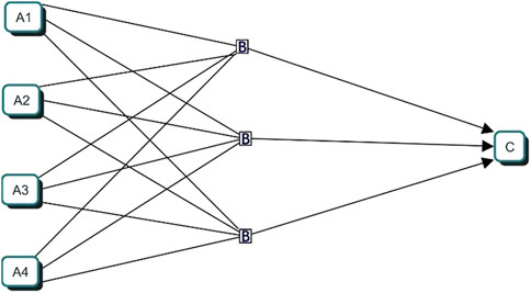
Figure 1. Proposed Neural Network Schematic.
Monthly precipitation data was collected for the period 2000–2015 from 49 stations registered by the National Institute of Meteorology and Hydrology (INAMHI), then the information was evaluated and reclassified, selecting those stations with at least 70% of the selected period; this criterion was used to have a representative number of stations for a reliable evaluation (Luna et al., 2018). In this way, the 24 stations that met this percentage of information were defined in Supplementary Table S1.
Three methodologies were used to fill in missing information, each of which was selected according to the number of data to be filled in and further characteristics as described below Figure 2.
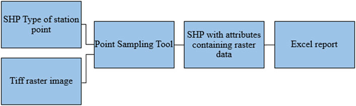
Figure 2. Scheme for the extraction of raster data.
This method constructs a linear model represented by the “x” independent variable and “y” dependent variable. When the
Where:
This method was used to fill stations with information that was missing by no more than 10% and to maintain a station with similar characteristics that could be used as a base station.
It is an average that considers the inverse of the squared distance as a weighting factor, thus distributing the contribution of each auxiliary station by weight, based on Eq. 2 (Chow et al., 1994), cited by (Toro et al., 2017).
Pm = precipitation is generated for the station to be filled in.
P1, P2, P3 = Monthly precipitation of each station in each quadrant.
D1, d2, d3 = Distance from each station to the station to be refilled.
1/d12 = The weight applies to each station concerning the station to be filled in.
This model was used to fill in the data of stations that, as in the previous case, have a base station and do not exceed 10% of missing data.
The Neural Network (NR) corresponds to a mathematical modelling technique; its structure is represented as links through which information is transmitted between neurons, which finally deliver a result by mathematical functions (Ovando et al., 2005). This model was used to fill in the stations’ data with between 10% and 30% of missing information, using three stations with similar characteristics plus the station to be filled in. The proposed model presents three layers of neurons with forward propagation of information, and the activation function is in a linear category. Its composition corresponds to A (input neurons, data from each station), B (hidden neuron layer or processing unit) and C (output layer or predicted data). In simplified form, it corresponds to a predefined set of regressions with a defined number of iterations, resulting in the prediction of the missing data, 2.
The NR was trained with the help of the Sklearn Python library, a set of routines for predictive analytics that includes classifier algorithms, regression and clustering algorithms, among others (Pedregosa et al., 2019).
Once the data from the 24 stations was complete, an exploratory graphic analysis was conducted to verify trends and changes in the time series (Carvajal and Castro, 2010). The double mass curve graph was used in this analysis, which compares the study series with a standard series resulting from the averages of the series to be analysed. If significant variations are identified in the series, i.e., there is a break in the slope, it must be adjusted. This adjustment is made using the corresponding slope ratio (Guevara, 2015), based on Eq. 3:
The accumulated series were defined in seven groups of stations, given that the climatic, hydrographic and topographic conditions are variable throughout the study area and that the stations under analysis are dispersed over it so as not to cause errors and distortions. Considering the above, the criteria for grouping were climatic similarity, altitude and hydrographic unit, Supplementary Table S2.
Hydrological processes evolve in space and time in a partially predictable and random way. Hence, these are stochastic processes. Various probabilistic distribution functions have been used to describe such behaviour. Although most hydrological models assume a normal distribution, it is necessary to test whether or not to reject the null hypothesis that the data distribution follows this type of theoretical distribution. In this study, the Kolmogorov Smirnov (K-S) test was used to validate the fit of the theoretical function. To carry out the confirmatory analysis, there are several parametric and non-parametric statistical tests; the use of one or the other depends on whether or not the theoretical assumption of normal distribution of the data is fulfilled (García et al., 2010). Parametric tests assume that the data distribution is normal and sensitive to the amount of data, skewness, and outliers. On the other hand, non-parametric tests do not require any assumption of known distribution, which indicates that they are helpful for a wide range of distributions.
Corresponding to a parametric test that relates the variances of two sets of data, these sets are the result of dividing the series to be evaluated into two groups, based on Eq. 4 and Eq. 5.
The test is rejected if F is in:
This is a non-parametric test to determine whether two samples differ in relation to their medians (Gómez, Danglot, and Vega, 2003). The overall median value is determined by combining the values of each sample, as shown in Supplementary Table S3. Then, it is determined in each sample how many higher and lower values exist concerning the overall median (Badii et al., 2012), cited by (Valencia et al., 2020).
It is a parametric test that evaluates two sets of data resulting from dividing the series to be evaluated into two groups. The test requires that the variances are not significantly different. It is rejected if T falls within the rejection region for a significance level of
This is the non-parametric alternative to comparing two independent averages via Student’s t-test. The test’s null hypothesis is that the two samples of size
Samples A and B are identified, with N and M observations. The observations are ordered as if they were a single sample and ordered ranges of values are assigned. Subsequently, the values belonging to each sample are identified, and the sums of each sample’s ranges are calculated, thus defining S, which corresponds to the sum of ranges of the most negligible value in (Badii et al., 2012) cited by (Valencia et al., 2020).
The satellite data evaluated in this work corresponds to GPM’s Integrated Multi-Satellite Retrievals algorithm in its version 06 (IMERG). The data corresponds to monthly accumulated precipitation estimates at a spatial resolution of 0.1° per pixel. To download it, you must fill out the registration form on the portal https://urs.earthdata.nasa.gov. Once registered, you can access it with your username and password. Once inside the server, in the Select Plot tab, locate the type of map to consult. In our case, it is the accumulated map; select the temporal space where you want to download the information in the Select Date Range. For the present work, it will be monthly: in Select Region, locate the area from where you want to download the information; for this work, a box was marked between the coordinates −80.5298, −5.0427 and −78.8928, −3.3838. At the bottom, in the Keyword box, we place the variable to be searched for, precipitation. Finally, all the information available on the server is displayed, and we can choose according to the user’s requirements, as it can be differentiated by units, resolution, dates, and type of algorithm or satellite.
For the present work, 187 Tiff files were obtained, one for each month and one for each year. To complete the analysis period, the months from January to May 2000 were completed with the weighted averages of the other years, as the satellite information available corresponds to June 2000. Once the raster information had been downloaded, a point-type ship of the 24 stations was produced, and the Point Sampling Tool, a tool for extracting the raster information to the ship attribute table in Supplementary Figure S3, was installed in QGIS software.
The statistical evaluation was performed for the uncorrected and corrected satellite products, and this validation was performed concerning the observed precipitation data. The statistical means used are the root mean square error (RMSE), the bias (RVB), the Nash-Sutccliffe coefficient (NS), the Pearson coefficient (R) and the coefficient of determination (R2). The RMSE quantifies the magnitude of the deviation of the simulated values from the observed values. The BVR quantifies the extent to which the simulated data overestimate or underestimate the expected value of precipitation (Shahid et al., 2021). A positive value indicates overestimating the amount of rainfall, while a negative value indicates underestimation. The NS measures how much of the variability of the observations is explained by the estimate in Supplementary Table S4. Finally, R expresses the linear dependence between observed and simulated values over time (Guachamín et al., 2019).
Satellite precipitation estimates are commonly affected by random and systematic errors (bias) (Mendez, 2016). The present work used a multiplicative correction factor through the Inter-Sectoral Impact Model Intercomparison Project (ISIMIP) method. The method preserves relative changes in monthly precipitation values. In addition to the monthly correction, the method also corrects for daily variability on the monthly mean; however, this detail is not explored in the present work as no daily scale data is being analysed.
Given the temporal and spatial variability of precipitation, the method uses a multiplicative correction factor, a function of the observed statistical series (the more data, the more optimal the C factor). To avoid discrepancies between the observed and corrected data series, the C factor has an upper limit of 10 to avoid very high corrected values. This can occur when the observed series are too short to approximate statistical parameters (Hempel et al., 2013). The following expression gives the fit of the satellite estimates, based on Eq. 9:
The following equation will adjust the daily precipitation data once the C-factor is defined, based on Eq. 10.
This correction is applied to the grid point closest to the station point. Interpolation techniques generally underestimate high-intensity rainfall and overestimate low-intensity rainfall (Bohling and Wilson, 2006).
Once the available data quality analysis has been carried out, Figure 1 defines the network of rainfall stations that will be used to evaluate satellite precipitation products.
The linear correlation method, a widely used technique, is instrumental in estimating the monthly and annual data of the study stations. However, its effectiveness relies on the presence of a nearby station, known as an auxiliary station, with consistent and observable data. This auxiliary station plays a crucial role in establishing a linear correlation and regression between the station with missing data and itself. By doing so, we can extend the record of the meteorological station based on the available information between the years 2000–2015. The more extensive the record or series of values observed in this auxiliary station, the more accurate the estimates and statistical inferences based on such data will be (Herrera et al., 2017).
The results presented in the table above show that the models fit the data. The coefficient of determination represents the percentage of variation in the response variable, which a linear model explains. In other words, there is a good correlation between the data (Toro et al., 2017), which obtained similar results when filling in missing data using the linear correlation method for the Ambi River basin.
The summary of the fit by the linear correlation method for stations with up to 10% missing data is presented in Supplementary Table S5.
This method consists of applying an average with the inverse of the squared distance that will act as a weighting factor; in addition, it is necessary to the deductive rationale based on the percentage of participation that the missing data has over the other available monthly data, in addition, the dependent meteorological variable is the value of the missing data in the station. The independent ones are the value of the variable of the auxiliary stations (Campos, 1998).
United States National Weather was applied to stations M0432 and M0142; given that there were no auxiliary base stations to apply the linear correlation method and that the data to be completed is less than 10%, this method was decided upon. In addition, station M1161 was used to apply the model after verifying the respective data based on Supplementary Table S6.
The precipitation values obtained by this method are quite stable concerning the existing statistics since, as will be analysed later in the double mass plot, both stations showed good consistency. They passed the statistical tests of confirmatory analysis.
The missing data adjustment by this methodology consisted of using three auxiliary stations plus the station to be completed. The training of the NR can be carried out considering several criteria since the meteorological precipitation data adopted were climatic similarity between stations, distance, altitude and preferably that they are within the same hydrographic system.
Supplementary Figure S4–S13 shows the results obtained for the ten stations that completed the missing data by this method. The graphs show the annual distribution of precipitation at the auxiliary stations in green, the station to be completed in red and the station with complete data in blue. It can also be seen that the annual distribution for all the auxiliary stations shows a similar trend, which is evidence that a good selection criterion was used. It can also be seen that the complete station graphically shows good results, which are corroborated by the consistency analysis.
Once the data had been completed using the methodologies described above, the double mass graph was used to detect series with certain types of systemic errors due to data collection, changes in instrumentation, etc. The results show that 20 of the 24 stations have consistent data for the period evaluated. The results show that 20 out of 24 stations present consistent data for the period evaluated in Supplementary Figure S14–S36.
Stations M0435 in Supplementary Figure S37, M0544 in Supplementary Figure S38, and M0147 in Supplementary Figure S39 present a significant break in their slope, so an adjustment is necessary. This methodology did not evaluate station M0142 as it could not be incorporated into any group because it is located in another hydrographic demarcation.
The adjustment made to stations Alamor M0435 in Supplementary Figure S37, Colaisaca M0544 in Supplementary Figure S38, and Yangana M0147 in Supplementary Figure S39 is presented in the following graph: a) corresponds to the uncorrected data, b) to the slope break, and c) corrected data.
The graphs in Supplementary Figure S40–S63 show that the slope break disappears after adjustment. In other words, the adjusted series presents a stable relationship of proportionality and consistency.
Supplementary Table S7 presents the results of the Kolmogorov-Smirnov (K-S) test, which was performed to validate the fit of the theoretical function. A significance level of 5% (p-value = 0.05) was used as the threshold for judging whether a result is statistically significant.
Null hypothesis
The results in Supplementary Table S7 indicate that for all stations, the
Supplementary Table S7 also presents the results of the confirmatory tests. The median test showed that none of the stations presented statistically significant differences concerning the value of the measure of central tendency, concluding that the subgroups formed present identical statistical properties. On the other hand, the Mann-Whitney U test shows that, for all stations, the subgroups formed have similar distributions, i.e., they are statistically equivalent in their position.
The statistical metrics between the observed and estimated data without correction show graphically that the 24 stations evaluated show a trend concerning the annual rainfall distribution. However, the observed values are higher than the simulated values. Although they show a similar trend, there is a deviation between the observed and simulated values, which is confirmed by the RMSE values that range from 34 to 157, as shown in Supplementary Table S8.
Supplementary Figure S40–S63 graphically show the annual trend of observed and estimated rainfall for the 24 stations analysed. If we look at Supplementary Table S1, where the altitude is presented, and Supplementary Figure S1, where the distribution of the analysed stations is given, it can be seen that the stations located in the lower part (example M0151; 223 m. a.s.l) of the study area present a defined distribution during the year, that means with months of high concentration and months of low or no rainfall.
This differs from the stations in the upper part (example M0432; 2,525 m. a.s.l), where precipitation variability during the year is observed.
Considering the above and observing the data in Supplementary Table S9, it must be evident that the IMERG estimated data present a better adjustment on the stations in the low zone and defined seasonality concerning the stations in the high zone and with variable seasonality, or vice versa. In other words, the altitudinal difference and the seasonal variation are not factors that condition a high or low performance of the estimates of the satellite products analysed in this work since, for both scenarios, the adjustment is similar.
One thing to consider from the results presented is that stations M0147 and M0432 are the least well-adjusted according to the statistical parameters.
Supplementary Table S9 presents the bias correction performance between observed and estimated data for the methodology proposed in this paper.
Using the correction factor obtained for each station and each month from Supplementary Table S9 significantly improves the simulated data. The data simulated by IMERG without correction present an underestimation in most stations concerning the observed data. However, once the correction is made, it is evident that the RVB tends to zero, i.e., there is a better fit between the corrected and observed data.
The training of the neural network to complete missing data, according to the results obtained, is an interesting tool that provides good results for this specific case. Studies by (Muñoz et al., 2020) show promising results in estimating meteorological data through NR. However, it should be pointed out that the training parameters of the NR are entirely different for each case. This opens up infinite possibilities and tools that can be incorporated for these types of analysis, like Supplementary Figure S4.
Part of the confirmatory analyses carried out can be seen from the results obtained in Supplementary Table S7, as well as in the studies carried out by Carvajal and Castro, after analysing the probabilistic distribution of the data, have evaluated various parametric and non-parametric tests, as well as graphical analyses, and concluded that graphical tests and confirmatory statistical analyses are essential tools in the exploratory analysis of data.
In the statistical indicators of efficiency in the results obtained in Supplementary Table S8 and as indicated by (Molnar et al., 2020) in Supplementary Table S4, the NS values for the stations evaluated range from satisfactory to good. The RVB is negative, i.e., there is an underestimation between the observed and simulated data, and the R coefficient presents values between 0.6 and 0.93, indicating a correlation between the observed and simulated values.
If we visualise Supplementary Figure S4, we can identify that these are closer to the eastern mountain range; that is, by analysing this scenario, the IMERG data present a low adjustment concerning those observed in areas close to the Amazon. The above results are similar to those obtained by (Mendez, 2016), where the IMERG products represent very well the temporal variability in a region of Chile. Also, Zulkafli compared the TRMM V6 and V7 products with data from rain gauges in the northern region of Peru and southern Ecuador, resulting in an underestimation between the estimated and observed data in the western regions of the Andes. Both of these studies are somewhat related to the present work.
It is important to emphasise that to compare results with other regional studies. It is necessary to consider the conditions under which they have been carried out, given that, as stated by (Wang and Wolff, 2012) in their study on the evaluation of TRMM products in Central Florida, these results cannot apply to other regions as there are determining factors such as the rainfall regime and the spatial and temporal scale that define the conditions of a region.
Likewise, the NS is between 0.36 and 0.89, and the Pearson coefficient is between 0.6 and 0.91. What contrasts with these results are the high RMSE values, which are between 104 and 25. These RMSE error values can be associated with the analysis level, as data are being analysed monthly. These results are also similar to those obtained by (Ramoelo et al., 2013).
Based on the data obtained in this study, we seek to make a significant contribution to water resource management and decision-making; by estimating the calculation of missing data, we seek to have more accurate hydrological modelling; this can be used in the future to predict the behaviour of water bodies, reservoir levels and the flow of water bodies such as rivers, lakes and lagoons near the study area, in order to have more accurate planning of water management and to give a better response to possible extreme weather events (Minga et al., 2018).
Estimates of precipitation data are essential for drought monitoring in the study area; with these results, there is more reliability on the amount and distribution of precipitation in order to detect early and accurately the drought conditions that may occur, thus contributing to a faster response to mitigate the impacts that are generated and may come to affect the needs of different sectors such as agriculture, industry and domestic consumption within the province of Loja (Aguirre et al., 2015).
1. In the present work, the satellite products corresponding to the IMERG V06 algorithm were evaluated using rainfall data from selected monthly scale stations for the province of Loja in southern Ecuador. Four statistical efficiency indicators were used for this evaluation: mean square error, bias, Nash-Sutccliffe coefficient and Pearson coefficient. Previously, the statistical series of observed data were analysed and adjusted.
2. The use of various methodologies for adjusting missing data allowed better adjustment of the information and, consequently, better results. This allowed a broader approach according to each situation.
3. The exploratory graphical analysis applying the double mass curve identified consistency in the statistical series of 20 of the 23 stations evaluated by this method. In addition to identifying that the series of three stations presented inconsistencies, it allowed the adjustment of these series, thus obtaining a series suitable for subsequent analyses.
4. The application of non-parametric statistical tests such as the Median and the Mann-Whitney U test helps to confirm the exploratory graphical analysis, which in turn allows us to have confidence in the statistical series to be used for further analysis.
5. The results show good performance of the uncorrected satellite products with R coefficients between 0.55 and 0.93 and NS from 0.21 to 0.66. The RVB presents underestimates between simulated and observed values and RMSE values of 157 and 24.
6. The IMERG underestimates rainfall in most of the 24 stations evaluated, except for stations M0759, M0760, M0143, M0145, and M0147, where a slight overestimation is evident in both cases without exceeding unity.
7. Applying the correction factor in general terms significantly improved the simulated data, obtaining values of R between 0.6 and 0.95, NS, 0.5 to 0.91, RVB -0.007 and 0. The high values of RSME are associated with the assessment being carried out on a monthly scale.
8. The performance of the evaluated satellite products does not vary at the altitudinal level nor the temporal level; the results show that their performance is similar in both scenarios. Suppose it has been identified that the performance is lower when approaching the Amazon region of Ecuador. In that case, this result should be corroborated with more detailed information since, in this work, only two stations were close to this region, and the data obtained from them allowed us to reach this conclusion.
9. The results show that the methodology applied for correcting the simulated data performed well; however, it is recommended that an evaluation with daily scale series be carried out to obtain better results.
The raw data supporting the conclusion of this article will be made available by the authors, without undue reservation.
LV: Writing–original draft, Software, Methodology, Investigation, Data curation. CA: Investigation, Supervision, Writing–review and editing. DG: Data curation, Writing–review and editing, Visualization.
The author(s) declare that no financial support was received for the research, authorship, and/or publication of this article. The authors declare that the funds used in this research project were their own; it does not involve an external institution or entity.
The authors declare that the research was conducted in the absence of any commercial or financial relationships that could be construed as a potential conflict of interest.
All claims expressed in this article are solely those of the authors and do not necessarily represent those of their affiliated organizations, or those of the publisher, the editors and the reviewers. Any product that may be evaluated in this article, or claim that may be made by its manufacturer, is not guaranteed or endorsed by the publisher.
The Supplementary Material for this article can be found online at: https://www.frontiersin.org/articles/10.3389/fenvs.2024.1408866/full#supplementary-material
Aguirre, N., Eguiguren, P., Maita, J., Samaniego, N., Ojeda, T., and Aguirre, Z. (2015) “Vulnerabilidad Al cambio climático en La región sur del Ecuador: potenciales impactos en los ecosistemas,” in Producción de Biomasa y Producción Hídrica. Universidad Nacional de Loja y Servicio Forestal de los Estados Unidos. Loja. Available at: https://biblioteca.uazuay.edu.ec/buscar/item/83231.
Alvarez-Mendoza, C. I., Teodoro, A. C., Torres, N., and Vivanco, V. (2019). Assessment of remote sensing data to model PM10 estimation in cities with a low number of air quality stations: a case of study in quito, Ecuador. Environments 6 (7), 85. doi:10.3390/environments6070085
Andrade, O. (2016). Evaluación de Imágenes Satelitales de Precipitación GPM (Global Precipitation Measurement) a Escala Sub-Diaria Para La Provincia Del Azuay. Available at: http://dspace.ucuenca.edu.ec/handle/123456789/24214.
Badii, M., Guillen, A., Araiza, L., Cerna, E., and Valenzuela, J. (2012). Métodos No-Paramétricos de Uso Común. Daena Int. J. Good Conscience 6 (1), 132–155.
Berlanga, V., and Rubio, M. (2012). Clasificación de Pruebas No Paramétricas. Cómo Aplicarlas. Rev. d’Innovació i Recer. En. Educ. 5, 101–113. doi:10.1344/reire2012.5.2528
Bohling, G., and Wilson, B. (2006) Statistical and geostatistical analysis of the Kansas high plains water table elevations, 2007 measurement campaign. Kansas Geological Survey. Available at: https://www.kgs.ku.edu/Hydro/Levels/2006/OFR06_20/.
Campos, D. (1998) Procesos del ciclo hidrológico. Universidad Autónoma de San Luis Potosí. Available at: https://bit.ly/3GOKZdS.
Carrera, V., Guevara, P., Tamayo, L., Balarezo, A., Narváez, C., and Morocho, D. (2016). Relleno de series anuales de datos meteorológicos mediante métodos estadísticos en la zona costera e interandina del Ecuador, y cálculo de la precipitación media. IDESIA (Chile) 34:(3), 81–90. doi:10.4067/S0718-34292016000300010
Carvajal, Y., and Castro, L. (2010). “Análisis de tendencia y homogeneidad de series climatológicas,” in Ingeniería de Recursos Naturales y Del Ambiente, 15–25. Available at: https://www.redalyc.org/articulo.oa?id=231116434002.
Chow, V.Te, Maidment, D., and Mays, L. (1994). Hidrología aplicada. Available at: https://drive.google.com/file/d/1P_PNmXkAdqTn8GihnKUWZu_YYyUt2Q3k/view.
de Loja, P. (2019) Consejo Nacional para la Igualdad de Género, Naturaleza y Cultura Internacional. Universidad Nacional de Loja, and Área de Sostenibilidad Urbana y Territorial de Tecnalia Research.
Díaz, M., Herrera, G., and Valdés, A. (2009). Un Modelo de Corregionalización Lineal Para La Estimación Espacial de La Precipitación En El Valle de La Ciudad de México, Combinando Datos de Pluviógrafos Con Imágenes de Radar Meteorológico. Ing. Hidráulica En. México 24 (3), 63–90.
García, R., González, J., and Jornet, J. M. (2010). “Pruebas No paramétricas. SPSS. Kolmogorov Smirnov,” in Grupo de Innovación Educativa (Universidad de Valencia), 1–5. Available at: http://www.uv.es/innomide/spss/SPSS/SPSS_0802A.pdf.
Gómez, M., Danglot, C., and Vega, L. (2003). Prevention of vasospasm by early operation with removal of subarachnoid blood. Rev. Mex. Pediatría 70 (2), 91–99. doi:10.1227/00006123-198203000-00001
Guachamín, W., Páez, S., and Horna, N. (2019). Evaluación de Productos IMERG V03 y TMPA V7 En La Detección de Crecidas Caso de Estudio Cuenca Del Río Cañar. Rev. Politécnica 42 (2), 31–48. doi:10.33333/rp.vol42n2.942
Guevara, E. (2015). “Métodos Para El Análisis de Variables Hidrológicas y Ambientales,” in Autoridad Nacional del Agua. Available at: https://catalogobiam.minam.gob.pe/cgi-bin/koha/opac-detail.pl?biblionumber=4011.
Hempel, S., Frieler, K., Warszawski, L., Schewe, J., and Piontek, F. (2013). A trend-preserving bias correction; the ISI-mip approach. Earth Syst. Dyn. 4 (2), 219–236. doi:10.5194/esd-4-219-2013
Herrera, C., Campos, J., and Carrillo, F. (2017). Estimación de Datos Faltantes de Precipitación Por El Método de Regresión Lineal: Caso de Estudio Cuenca Guadalupe, Baja California, México. Investig. Cienc. La Univ. Autónoma Aguascalientes 71, 34–44. doi:10.33064/iycuaa201771598
Hou, A., Ramesh, K., Neeck, S., Azarbarzin, A., Kummerow, C., Kojima, M., et al. (2014). The global precipitation measurement mission. Bull. Am. Meteorological Soc. 95, 701–722. doi:10.1175/BAMS-D-13-00164.1
Huffman, G., McCarty, W., Cosner, C., and Reed, J. (2022) MERG: integrated multi-satellite Retrievals for GPM. Available at: https://gpm.nasa.gov/data/imerg.
Huffman, G. J., and Adler, R. (2023). Algorithm theoretical basis document (ATBD) for global precipitation climatology project version 3.0 precipitation data. Greenbelt, MD 29 (2019), 1–32. Available at: https://docserver.gesdisc.eosdis.nasa.gov/public/project/MEaSUREs/GPCP/GPCP_ATBD_V3.1.pdf.
Luna, A., Ramírez, I., Sánchez, C., Conde, J., Agurto, L., and Villaseñor, D. (2018). Spatio-temporal distribution of precipitation in the Jubones River basin, Ecuador: 1975-2013. Sci. Agropecu. 9 (1), 63–70. doi:10.17268/sci.agropecu.2018.01.07
Méndez, R. (2016). Productos de Precipitación Satelital de Alta Resolución Espacial y Temporal En Zonas de Topografía Compleja. Pontif. Univ. Cat´9olica Chile. Available at: https://repositorio.uc.cl/bitstream/handle/11534/21480/RUTHARACELLYMÉNDEZRIVAS.pdf?sequence=1.
Minga, S., Gómez, M., Bâ, K. M., Balcázar, L., Manzano, L., Cuervo, A., et al. (2018). Estimation of water yield in the hydrographic basins of southern Ecuador. Hydrology Earth Syst. Sci. Discuss. 30, 1–18. doi:10.5194/hess-2018-529
Molnar, P., Battista, G., and Burlando, P. (2020). Modelling impacts of spatially variable erosion drivers on suspended sediment dynamics. Earth Surf. Dyn. 8 (3), 619–635. doi:10.5194/esurf-8-619-2020
Morrow, A. (2015). The TRMM rainfall mission comes to an end after 17 years. Available at: https://phys.org/news/2015-04-trmm-rainfall-mission-years.html.
Muñoz, W., Bedoya, O., and Rincón, M. (2020). Aplicación de Redes Neuronales Para La Reconstrucción de Series de Tiempo de Precipitación y Temperatura Utilizando Información Satelital. Rev. EIA 17 (34), 1–16. doi:10.24050/reia.v17i34.1292
Ovando, G., Bocco, M., and Sayago, S. (2005). REDES NEURONALES PARA MODELAR PREDICCIÓN DE HELADAS. Agric. Técnica 65 (1), 65–73. doi:10.4067/s0365-28072005000100007
Pedregosa, F., Varoquaux, G., Gramfort, A., Vincent, M., and Bertrand, T. (2019). Generating the blood exposome database using a comprehensive text mining and database fusion approach. Environ. Health Perspect. 127 (9), 2825–2830. doi:10.1289/EHP4713
Ramoelo, A., Skidmore, A. K., Cho, M. A., Mathieu, R., Heitkönig, I. M. A., Dudeni-Tlhone, N., et al. (2013). Non-linear partial least square regression increases the estimation accuracy of grass nitrogen and phosphorus using in situ hyperspectral and environmental data. ISPRS J. Photogrammetry Remote Sens. 82, 27–40. doi:10.1016/j.isprsjprs.2013.04.012
Shahid, M., Rahman, K.Ur, Haider, S., Gabriel, H. F., Khan, A. J., Pham, Q. B., et al. (2021). Assessing the potential and hydrological usefulness of the CHIRPS precipitation dataset over a complex topography in Pakistan. Hydrological Sci. J. 66 (11), 1664–1684. doi:10.1080/02626667.2021.1957476
Toro, A., Arteaga, R., Vázquez, M., and Ibáñez, L. (2017). Relleno de Series Diarias de Precipitación, Temperatura Mínima, Máxima de La Región Norte Del Urabá Antioqueño. Rev. Mex. Ciencias Agrícolas 6 (3), 577–588. doi:10.29312/remexca.v6i3.640
Valencia, E., Caiza, E., and Bedoya, M. (2020). Investment decisions and profitability under the financial valuation in the large industrial companies of the cotopaxi province, Ecuador. Revista Universidad Empresa 22 (39), 1–26. Available at: https://revistas.urosario.edu.co/index.php/empresa/article/view/8099/8615.
Wang, J., and Wolff, D. B. (2012). Evaluation of TRMM rain estimates using ground measurements over central Florida. J. Appl. Meteorology Climatol. 51 (5), 926–940. doi:10.1175/JAMC-D-11-080.1
Keywords: estimation, IMERG, precipitation, satellite products, water resources
Citation: Valverde L, Álvarez CI and Gualotuña D (2024) Remote sensing-based estimation of precipitation data (2000-2015) in Ecuador's Loja province. Front. Environ. Sci. 12:1408866. doi: 10.3389/fenvs.2024.1408866
Received: 28 March 2024; Accepted: 06 May 2024;
Published: 03 June 2024.
Edited by:
Srdan Kostic, Jaroslav Černi Water Institute, SerbiaReviewed by:
Muhammad Shahid, Brunel University London, United KingdomCopyright © 2024 Valverde, Álvarez and Gualotuña. This is an open-access article distributed under the terms of the Creative Commons Attribution License (CC BY). The use, distribution or reproduction in other forums is permitted, provided the original author(s) and the copyright owner(s) are credited and that the original publication in this journal is cited, in accordance with accepted academic practice. No use, distribution or reproduction is permitted which does not comply with these terms.
*Correspondence: Dayana Gualotuña, Y2FsdmFyZXptQHVwcy5lZHUuZWM=
Disclaimer: All claims expressed in this article are solely those of the authors and do not necessarily represent those of their affiliated organizations, or those of the publisher, the editors and the reviewers. Any product that may be evaluated in this article or claim that may be made by its manufacturer is not guaranteed or endorsed by the publisher.
Research integrity at Frontiers
Learn more about the work of our research integrity team to safeguard the quality of each article we publish.