Identification of optimal CMIP6 GCMs for future typical meteorological year in major cities of Indonesia using multi-criteria decision analysis

Many studies often use a single global climate model (GCM) across multiple cities to develop future Typical Meteorological Year (TMY), without emphasizing city-specific selection of GCM. The present investigation employs the Analytical Hierarchy Process (AHP) to assess city-specific GCMs for generating future TMY datasets across 29 Indonesian cities. Six GCMs from the coupled model intercomparison project phase 6 (CMIP6) were evaluated against Modern-Era Retrospective Analysis for Research Applications (MERRA-2) to assess their performance in simulating surface air temperature, precipitation, wind speed, and relative humidity. Six statistical measures were used to recognize the systematic biases. Further, AHP was applied to integrate these statistical measures to calculate the city-specific total relative error for each meteorological parameter. Results of total relative error show that TaiESM, 6-Model Ensemble (6ME), NorMM, and MPI-HR were best for simulating surface air temperature, precipitation, wind speed, and relative humidity in most cities, respectively. TMY recognizes distinctive importance among meteorological parameters. Thus, it is essential to reflect the parameter-specific importance while selecting GCMs for future TMY. Hence, AHP was reapplied on total relative errors accounting for differing weights of each meteorological parameter. Outcomes show that TaiESM, 6ME, and MPI-HR were found suitable for generating future TMY datasets in 18, 5, and 3 cities, respectively, while MPI-LR, NorLM, and NorMM were recommended for Boven Digoel, Medan, and Bengkulu cities, respectively. Using city-specific GCMs ensures precise and cost-effective future TMY generation, assisting urban planners and policymakers in designing environmentally sustainable buildings for anticipated climatic changes.

1 Introduction

Climate change is the persistent alteration of global or local climate conditions over an extended period. Alterations in climate are mainly identified by measuring the variations in meteorological factors, including temperature, precipitation, and other parameters (Gleick, 1986; Zhang et al., 2011). According to the Intergovernmental Panel on Climate Change (IPCC) fifth assessment report, from 1951 to 2012, the average global surface air temperature of the land and ocean has risen by 0.72°C (Stocker, 2014). By the end of the 21st century, it will increase to 1.8°C–4°C (Field, 2014). This report also applauds substantial greenhouse gas cuts, advocating for net zero emissions by mid-century to limit global temperature increase to under 1.5°C. As reported by various authors, urbanization is anticipated to drive a future rise in urban air temperatures (Vinayak et al., 2021; 2022; Bhanage et al., 2023a). The urbanization process also amplifies greenhouse gas (GHG) emissions, making the urban environment one of the prior concerns in the present world order (Ambade et al., 2021; Gautam et al., 2021; Thapliyal et al., 2022). These predictions of forthcoming changes in the climate bring noteworthy consideration to the research topics that highlight the paths to cut down on GHG emissions.

Buildings now contribute 33% of GHG emissions and 40% of global energy use, projected to rise by 61% by 2,100 (Santamouris, 2016; Teske et al., 2021). To restrict building energy consumption, the design of a building should pass the building energy consumption test to check whether the design of a building meets the criteria of energy savings. Building designs with accurate meteorological data, specifically Typical Meteorological Year (TMY) datasets, is essential in this testing. TMY dataset is a set of meteorological data representing the typical hourly weather conditions for a specific location over 1 year. These datasets represent local climate conditions for simulations. However, future climate changes make historical and present TMYs inadequate. Thus, creating TMYs considering future climate possibilities is vital. The most adopted approach for preparing future TMY datasets is morphing (Dias et al., 2020). The morphing method mainly relies on delta change in monthly means of the weather data to illustrate future weather; still, various studies reveal that weather variability and extreme events are not replicated by variations in monthly means (Dias et al., 2020). Apart from that, the morphing method also induces the effects of climate change independently between variables. Therefore, the most reliable methodology for constructing the future TMY dataset is to dynamically downscale the global climate models (GCMs). Compared to the morphing technique in a dynamical downscaling of GCMs, it captures a more detailed representation of physical processes, including atmospheric dynamics, land-surface interactions, and local feedback mechanisms, contributing to a more accurate representation of future climate conditions.

The GCMs are numerical models that simulate the global climate’s preceding, contemporary, and forthcoming conditions (Alizadeh, 2022). The sixth coupled model intercomparison project (CMIP6) provides a climatic dataset from more than 30 GCMs developed by various organizations. It is necessary to assess the proficiency of these GCMs in replicating essential climate variables by comparing their outputs with observed or reanalysis data. Depending upon several factors, such as parameterization schemes, grid size, representation of the earth system, and initial and boundary conditions, each GCM exhibits different uncertainties. However, using the climatic data by integrating all the GCMs may not always be suitable. The use of many models leads to increased ambiguities due to low simulation accuracy and process algorithms of ensemble members. Therefore, to generate the future TMY from individual GCMs, it is vital to compare each GCM or to identify the relative performance of each GCM based on different criteria that suit the TMY generation approach.

In recent years, numerous studies have explored the intricacies of climatic features in various regions, aiming to predict future climate scenarios. These investigations involve a meticulous evaluation of GCMs against observed or reanalysis data. For example, over Indian subcontinent, the exceptional performance of an ensemble comprising KIOST-ESM, MRI-ESM2-0, MIROC6, NESM3, and CanESM5 for maximum temperature and E3SM-1-0, NESM3, CanESM5, GFDL-CM4, INM-CM5-0, and CMCC-ESM2 for minimum temperature has been reported (Rahman and Pekkat, 2024). In the case of Indonesia, the superiority of the multi-model ensemble in simulating extreme precipitation events was noted (Kurniadi et al., 2023). A recent research over Guatemala located in central American region noted that MRI-ESM-2.0 and IPSL-CM6A-LR GCMs as the top performer for simulating surface air temperature and precipitation (Rivera, 2023). Research carried out in 2023, evaluated the performance 27 GCMs derived from CMIP6 over Southeast Asian territory, identified TaiESM as a most exceptional performer (Pimonsree et al., 2023).

While these studies primarily aimed to assess the GCMs’ proficiency in capturing large-scale spatial and temporal climate patterns, including regional temperature trends and precipitation variability, it is essential to emphasize that when evaluating GCMs for constructing future TMY data, a more focus on the local-scale characteristics of the climate becomes imperative. Thus, it is crucial to recognize that the approach adopted for regional-scale model evaluations may not necessarily be suitable for the meticulous preparation of future TMY datasets.

In past, numerous studies have been conducted to prepare the future TMY dataset from the GCMs (Haase et al., 2011; Nik, 2016; Huld et al., 2018; Troup et al., 2019; Yuan et al., 2022). However, to generate the future TMY, the criteria used to select GCMs differ in different studies. In 2011, after statistical evaluation of surface air temperature and precipitation acquired from six GCMs, Chan (2011) utilized the MIROC6-2-Med to simulate future TMY data over the entire Hongkong region. In 2022, Doutreloup et al. (2022) generated the future TMY dataset over Belgium using three climate models, namely, BCC-CSM2-M, MPI-ESM 1.2, and MIROC6. Jiang et al. (2019) used the HadCM3 data to generate the future TMY over eight different cities of the globe. Ji Wei Zhou (2022) used the Coordinated Regional Downscaling Experiment to estimate the future reference years over different Canadian cities. Bass et al. (2018) created a TMY dataset for Maricopa, Arizona, using six GCMs without evaluating their performance. Similarly, Manapragada et al. (2022) used the Canadian Earth System Model to generate future TMY data over Delhi, India without comparing different GCMs.

However, there are some limitations to these studies especially while selecting the GCMs for the development of future TMY dataset. First, some of the above studies have used a unique GCM to develop the future TMY dataset over different cities. But, some studies recently have shown that the performance of GCMs in simulating the different meteorological variables and phenomena varies concerning the cities (Bhanage et al., 2023b; VR, 2023). Second, many of the above-mentioned studies do not evaluate the performance of GCMs before adopting them for the development of future TMY dataset. Evaluating the performance of GCMs helps identify their strengths and weaknesses, allowing for the selection of models that better capture the local climate variability, which is essential for TMY dataset generation (Fildes and Kourentzes, 2011; McSweeney et al., 2015; Ruane and McDermid, 2017; Chowdhury and Behera, 2019) Third, in creating TMY data, it is imperative to recognize that different meteorological parameters have varying levels of importance. Yet, the studies mentioned above did not consider the respective significance of these parameters while selecting an appropriate GCM for future TMY development.

To overcome these limitations, the principal objective of this study is to develop a new framework for identifying GCMs tailored to the local climatic characteristics of each of Indonesia’s 29 cities to generate future TMY datasets. This study’s distinctive feature lies in its pioneering method for GCM selection, as it recognizes the diverse levels of significance attributed to individual meteorological and statistical parameters. Therefore, while identifying the city-wise optimal GCMs for preparing future TMY data, according to the author’s knowledge, this study will be a pioneering effort that considers the AHP-based multi-criteria decision analysis (MCDA) approach to incorporate and aggregate the subjective judgments associated with various meteorological and statistical parameters that allow a more transparent decision process.

The paper is structured into six distinct sections. The first section explores the research problem’s context, underscoring its significance, and outlines the study’s objectives. The second section offers comprehensive information about the study area. The third section delves into the research design and methodology employed in the study. The fourth section presents the study’s outcomes, encompassing data analysis, statistical insights, and other pertinent information related to the findings. The fifth section is dedicated to interpreting and comparing the results with previous studies. Finally, the sixth section summarizes the key findings, addresses limitations, and discusses the future scope of the study.

2 Study area

The present study has been conducted over twenty-nine major cities located in Indonesia (Figure 1). The overall area of Indonesia extends from the latitudes 11°S and 6°N and longitudes 95°E and 141°E. The elevation of the Indonesian region varies from 0 m to 3,505 m. Indonesia experiences a hot-humid tropical climate. The surface air temperature in Indonesia stays relatively constant throughout the year. The country has two seasons: the wet season, from October to April, and the dry season, from May to September. Due to its tropical climate, the coastal plains experience an average surface air temperature of around 28°C.

FIGURE 1

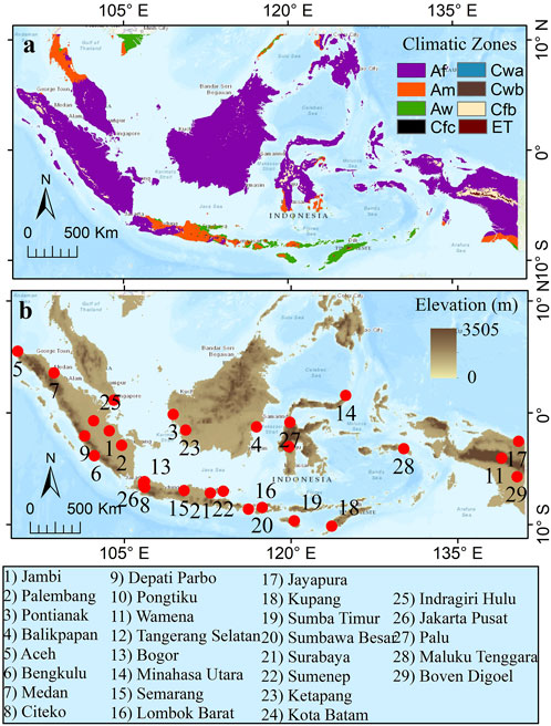
FIGURE 1. Study Area representing (A) Climatic zones of Indonesia based on Koppen -Geiger classification and (B) spatial variation in the elevation and the location of 29 major cities in Indonesia.

In comparison, the internal highland regions have a mean of 26°C, and the higher highland regions have temperatures around 23°C. The country’s relative humidity is very high and fluctuates between 70% and 90%. Indonesia experiences ample annual precipitation ranging from the driest regions of around 500 mm to more than 3,000 mm in the wettest regions (Kurniadi et al., 2023). It highlights the spatial heterogeneity in the precipitation over Indonesia. Given the spatial variabilities in temperature and precipitation across Indonesia, it is crucial to identify GCMs specific to each city for generating future TMY datasets.

3 Materials and methods

3.1 Data

The CMIP6 program includes historical (1850-2014) simulations based on observations and external forcings such as volcanic eruptions, solar variability, changes in GHGs, and aerosol concentrations (Eyring et al., 2016). In the CMIP6 stage, the scenarios of representative pathways (RCPs) i.e., RCP 2.6, RCP4.5, RCP 6.8 and RCP 8.5 of the CMIP5 have been apprised to shared socioeconomic pathways (SSPs) i.e., SSP1-2.6, SSP2-4.5, SSP4-6.0, and SSP5-8.5 respectively (Arnell et al., 2019; Gidden et al., 2019; Shiru and Chung, 2021). These SSP scenarios provide a framework for climate change research by describing plausible alternative futures of human development and greenhouse gas emissions. Each SSP scenario represents a different narrative about future socioeconomic conditions and policies. The SSPs encompass five different potentials: (a) a scenario characterized by growth and equality with a focus on sustainability (SSP1); (b) a condition where trends closely align with historical patterns (SSP2); (c) a world noticeable by resurgent nationalism and fragmentation (SSP3); (d) a scenario of intensifying global inequality; and (e) a state of rapid and unrestrained growth in both energy consumption and economic output (SSP5) (Shiru and Chung, 2021). The major goal of the CMIP6 program is to enhance the accuracy and reliability of climate models by incorporating improvements in emissions scenarios, land-use representation, physical process modeling, and model parameterization. This comprehensive approach allows for a more robust exploration of future climate conditions (Eyring et al., 2016). In the ongoing research, six historical GCMs were chosen to evaluate surface air temperature, precipitation, wind speed, and relative humidity. These GCMs were selected from the CMIP6 dataset, spanning the time frame from 1980 to 2014. The study utilizes MCDA-based statistical methods to perform a comparative evaluation between the chosen GCMs and reanalysis datasets.

The evaluation period from 1980 to 2014 was chosen because (i) the period of 1980–2014 serves as a reference period for climate agreement as it covers a large period of the recent past, (ii) the growing GHGs and anthropogenic influences marked this period of 1980 onwards, and (iii) as compared to earlier period (<1980), very few large-scale disturbances and the number of volcanic eruptions have increased between post-1980 period (Doocy et al., 2013). For this evaluation, 6 GCMs were selected based on the following criteria: (i) The GCMs must comprise the historical dataset of surface air temperature, precipitation, relative humidity, and wind speed from 1980 to 2014, (ii) the identical model should incorporate the climatological data from 2015 to 2,100 under SSP 5–8.5 scenario at 6 hourly interludes, and (iii) the model must have a forcing data from the r1i1p1f1 (first realization). Selection of the first realization ensures a fair and unbiased comparison across all GCMs, while the selection of the SSP 5–8.5 scenario is motivated by the chance it provides to gain insights into the potential extreme impacts of climate change. Detailed information on chosen GCMs is provided in Table 1.

TABLE 1

TABLE 1. Description of selected GCM data.

Subsequently, to assess the integrated performance, the selected GCMs, multi-model ensemble dataset (6ME), was calculated using Eq. 1 where i = different shortlisted GCMs.

$\left(\mathbf{6}\mathbf{M}\mathbf{E}\right)=\frac{\mathbf{1}}{\mathbf{n}}{\displaystyle {\sum }_{\mathbf{i}=\mathbf{1}}^{\mathbf{n}}}\text{GC}{\mathbf{M}}_{\mathbf{i}}(1)$

Further, this data has been compared with the monthly surface air temperature, precipitation, and relative humidity data obtained from the Modern-Era Retrospective Analysis for Research Applications (MERRA), Version 2 (Bosilovich, 2015). This dataset is established by incorporating ground-satellite observations and numerical model data. The spatial resolution of the MERRA2 dataset is 0.50 × 0.65. The flow of methodology is illustrated in Figure 2. After the acquisition of the MERRA-2 and selected CMIP6 GCMs, they were regridded to 1 × 1. This regridding process was performed to align the spatial resolution of the GCMs with the dataset, ensuring a consistent spatial framework for comparison. Furthermore, city-wise statistical analysis has been conducted to evaluate the performance of surface air temperature, relative humidity, precipitation, and wind speed derived from the MERRA-2 and CMIP6 GCMs, including the 6ME.

FIGURE 2

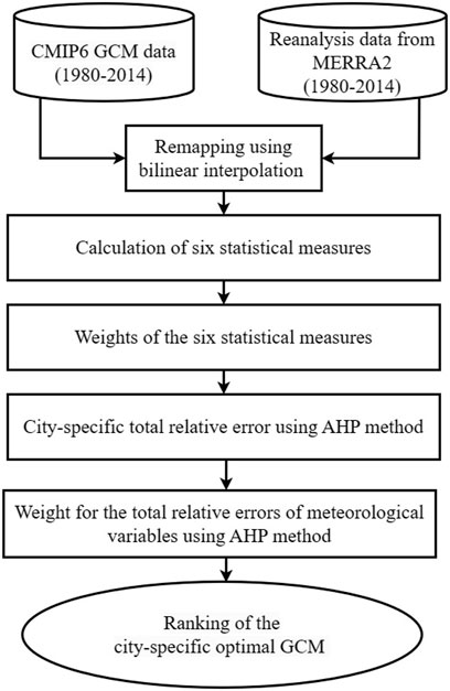
FIGURE 2. General flow of methodology adopted for identifying city-specific suitable GCMs for generating the future TMY dataset.

3.2 Statistical performance metrics

Several statistical performance metrics are generally utilized to evaluate the accuracy and reliability of the GCMs. Here, for each city, by comparing the MERRA-2 and GCMs, including the 6ME, six statistical metrics were calculated to analyze surface air temperature, precipitation, relative humidity, and wind speed as follows (see also Table 2 for their formula):

TABLE 2

TABLE 2. Details of six statistical measures.

The correlation coefficient (CC) depicts the strength of the association among the comparative dynamics of two variables; the values of the CC range from −1 to 1. The values closer to 0 (1 or −1) show the weaker (stronger) association between the two variables.

Standard deviation (SD) elucidates the dataset’s variation or dispersion. A lower standard deviation indicates that the values in the data are closer to the mean of the dataset. In contrast, higher standard deviation values imply that the dataset’s values spread wider.

Mean annual (MA) can calculate the sum of each mean annual divided by the total number of years. It is mainly used to estimate the shifts in the average annual values of each meteorological variable over the 29 cities.

Mean bias error (MBE) is the positive or negative difference between the dataset acquired from the reference and CMIP6 GCMs. MBE outcomes reveal whether the GCM simulations are warm or cold-biased compared with the reference data.

Mean seasonal cycle amplitude (SA) mainly highlights the difference between extremely hot and cold months that can be used to assess the gravity of alterations in surface air temperature, precipitation, wind speed, and relative humidity over the 29 cities considered for this study.

Root mean square error (RMSE) commonly measures the disparity between values simulated/predicted by a GCM and the reference. In other words, RMSE measures the error between simulated/predicted and reference datasets. The lower (higher) values of RMSE indicate the smaller (greater) error from the simulated/modeled values.

3.3 Relative weights by the analytical hierarchy process (AHP)

The quantitative assessment for the suitable GCMs for the generation of future TMY depends on multiple criteria, such as surface air temperature, precipitation, wind speed, and relative humidity. Also, statistical measures such as bias in SA, MBE, RMSE, CC, and bias in SD were used to generate the total relative error. This study employed the AHP method twice to ascertain the relative weights assigned to individual statistical measures and the total relative error calculated for each meteorological parameter.

Subsequently, the relative importance of each statistical measure (total relative error of every meteorological parameter) was established by administering questionnaires to a panel of 10 (8) experts. Detailed information regarding each questionnaire can be found in the Supplementary Material S1. The first step of the AHP process is the generation of the pairwise comparison matrix, where each criterion was compared to another using the Saaty Scale (Saaty, 1980) (see Table 3). In this study, the scale ranges between 1 and 5 based on the number of norms used to generate the total relative error and 1 and 4 for each meteorological parameter that can generate future TMY. The second step includes dividing each value in the matrix (C_ij) by the sum of columns in the pairwise comparison matrix to produce the normalized value (X_ij), as shown in Eq. 2.

${\mathit{X}}_{\mathit{i}\mathit{j}}={\mathit{C}}_{\mathit{i}\mathit{j}}/{\displaystyle \sum _{\mathit{i}=\mathbf{1}}^{\mathit{n}}}{\mathit{C}}_{\mathit{i}\mathit{j}}(2)$

TABLE 3

TABLE 3. Saaty Scale of relative importance and its corresponding description.

The third step is to generate the weight (W_ij) of each criterion, which is calculated by dividing the normalized value (X_ij) by the total number of criteria (n), as shown in Eq. 3.

${\mathit{W}}_{\mathit{i}\mathit{j}}={\displaystyle \sum _{\mathit{i}=\mathbf{1}}^{\mathit{n}}}{\mathit{X}}_{\mathit{i}\mathit{j}}/\mathit{n}(3)$

The last part of the AHP process is generating the consistency ratio (CR). The CR is used to determine whether each criterion’s weight is acceptable. It is acceptable if the CR value is less than or equal to 10% (0.10); otherwise, it is unacceptable. There are three sub-procedures to generate the CR. The first is to calculate the consistency measure (CM). CM can be calculated by multiplying the pairwise matrix with the weight (W_ij) and dividing the result by the weighted sum with the criterion weight. The consistency index (CI) is then calculated using Eq. 4, where the λ_max is the average of the CMs. Lastly, the CR is derived using Eq. 5, where the relative index (RI) value is shown in Table 4.

$CI=\left({\lambda }_{\mathit{max}}–n\right)/\left(n–1\right)(4)$

$CR=CI/RI(5)$

TABLE 4

TABLE 4. Random index matrix per number of criteria in decision-making.

3.4 City-specific ranking of the GCMs

For all the GCMs, the city-specific total relative error was calculated for each meteorological parameter. It was calculated by combining the five statistical measures computed in the above section. It reflects various attributes of model performance, such as biases, CC, and temporal changes. This thorough assessment enables a more extensive examination of GCMs. Calculating the total relative error to individual models based on performance enables an apparent evaluation and recognizes GCMs demonstrating comparatively better or poorer performance. The details of the methodology employed for the calculation of total relative error are as follows:

To determine the total relative error of the GCMs, we have incorporated all statistical metrics and assigned varying weights to each metric, which were obtained through the AHP. For a given model i and metric j, we first defined an error ${\mathrm{E}}_{\mathrm{I},\mathrm{j}}$ as

${\mathbf{E}}_{\mathbf{i},\mathbf{j}}=\left|{\mathbf{X}}_{\mathbf{\text{obs}},\mathbf{j}-}{\mathbf{X}}_{\mathbf{i},\mathbf{j}}\right|(6)$

where X_obs and X_i are the observed and simulated ensemble mean metrics, respectively, and the application of Eq. 6 included correlations (where X_obs necessarily equaled 1). Furthermore, relative error $E_{\mathrm{I},j}^{*}$ is defined as

${\mathit{E}}_{\mathbf{I},\mathit{j}}^{*}=\frac{{\mathbf{E}}_{\mathbf{i},\mathbf{j}}-\mathbf{min}\left({\mathbf{E}}_{\mathbf{i},\mathbf{j}}\right)}{\mathbf{max}\left({\mathbf{E}}_{\mathbf{i},\mathbf{j}}\right)-\mathbf{min}\left({\mathbf{E}}_{\mathbf{i},\mathbf{j}}\right)}(7)$

Then, for the calculation of total relative error, a weighted sum has been carried out concerning relative error estimated across all m metrics in Eq. 8

${\mathit{E}}_{\mathbf{I},\mathit{t}\mathit{o}\mathit{t}}^{*}={\displaystyle {\sum }_{\mathit{J}=\mathbf{1}}^{\mathit{m}}}{\mathit{W}}_{\mathit{j}}\ast {\mathit{E}}_{\mathbf{I},\mathit{j}}^{*}(8)$

to get the total relative error $E_{\mathrm{I},tot}^{*}$ per model. $W_j$ is the weight of each statistical metric j derived by using the AHP method. The values obtained for $E_{\mathrm{I},tot}^{*}$ are unitless. Finally, the models are ranked by their respective total relative error. Lower (higher) values of the $E_{\mathrm{I},tot}^{*}$ represents the higher (lower) suitability of the GCMs for an individual meteorological parameter over a specific city.

In the past, it was noted that the relative importance of meteorological parameters varies in the development of TMY datasets (Cebecauer and Suri, 2015; Li et al., 2021). Based on the methodology mentioned in earlier sections, weights for each climatic parameter were established for generating future TMY datasets ($W_{tmy}$). Further, to determine city-specific rankings of GCMs for future TMY creation, $E_{\mathrm{I},tot}^{*}$ Values were calculated for each meteorological parameter, and GCM for each city was combined with the corresponding. $W_{tmy}$ using Eq. 9. The outcomes of Eq. 9 yields unitless ranking scores depicted by ($\left.E_{\mathrm{I},rank}^{*}\right)$, enabling the determination of city-specific suitability of GCM for the future development of TMY. The resulting non-dimensional values, closer to 0 (1), indicate higher (lower) suitability of a GCM for developing future TMY datasets for a specific city.

${\mathit{E}}_{\mathbf{I},\mathit{r}\mathit{a}\mathit{n}\mathit{k}}^{*}={\displaystyle {\sum }_{\mathit{J}=\mathbf{1}}^{\mathit{m}}}{\mathit{W}}_{\mathit{t}\mathit{m}\mathit{y}}\ast {\mathit{E}}_{\mathbf{I},\mathit{t}\mathit{o}\mathit{t}\mathit{a}\mathit{l}}^{*}(9)$

4 Results

4.1 City-wise GCM performance

In statistical assessment for surface air temperature, precipitation, relative humidity, and wind speed, simulated monthly climatic data derived from 6 GCMs and one ensemble were compared with the MERRA-2 reanalysis data (1980-2014). Using different statistical measurements offers unique insights and helps evaluate different aspects of each GCM, allowing for a more robust analysis.

4.1.1 Surface air temperature

Figure3A–F represents the six statistical measures calculated for the surface air temperature over 29 cities of Indonesia. Here, MA surface air temperature obtained from the MERRA-2 and GCMs, including the 6ME, spans 290–302 K (Figure 3A). Based on the reanalysis data, Sumenep (Wamena) City recorded the highest (lowest) mean annual surface air temperature among all cities. In the case of Sumenep (Wamena) City, the magnitude of MA surface air temperature derived with MPI-LR (MPI-HR) exhibited close similarity when compared with the reanalysis dataset. The MBE of surface air temperature calculated from six GCM and 6ME varied between −3–5 K (Figure 3B). Considering the 6ME, out of 29 cities, 20 (9) cities show warm (cold) biases in mean annual surface air temperature. Among the 29 cities analyzed using the 6ME, 20 exhibit warm biases in mean annual surface air temperature, while 9 display cold biases. However, for other GCMs, biases vary depending on their specific tendencies. Regarding mean bias error, among 29 cities, 6ME was deemed suitable for 2 cities.

FIGURE 3

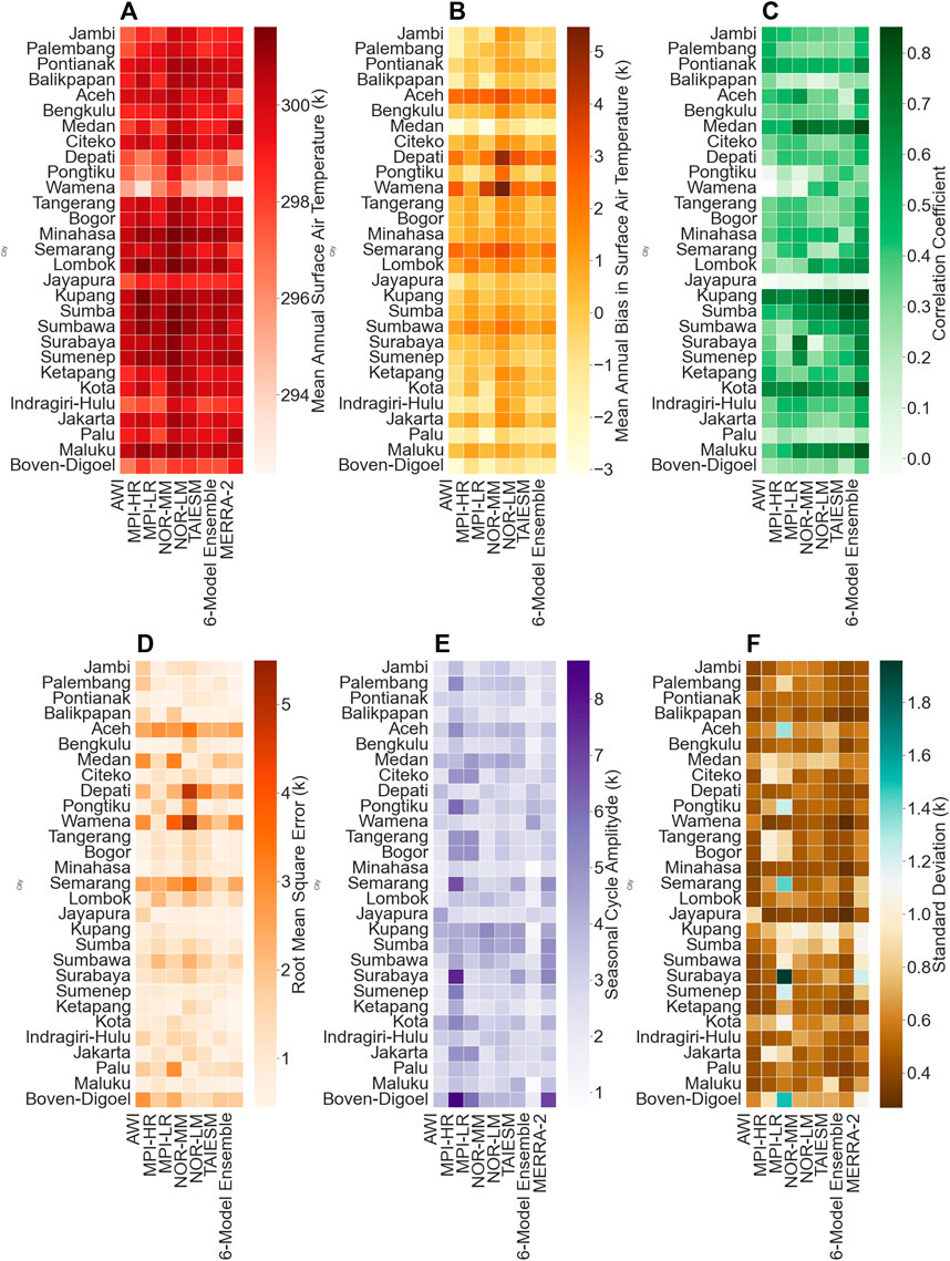
FIGURE 3. City-wise variation of different statistical metrics computed for surface air temperature across 29 cities in Indonesia (A) MA, (B) MBE, (C) CC, (D) RMSE, (E) SA, and (F) SD.

On the other hand, TaiESM exhibited exceptionally well over 11 cities in Indonesia. Figure 3C illustrates the variation in CC estimated for surface air temperature across different cities. The values of CC range from 0.3 to 0.85. Regarding CC, the performance of the 6ME was dominant in 20 cities. Further, the RMSE values computed by comparing each GCM and reanalysis dataset are illustrated in Figure 3D. For all the cities, the RMSE values range from 0.4 to 5.4 K. Considering the RMSE, 6ME (TaiESM) performance was better than that of 13 (9) cities. Figure 3E illustrates the city-wise alterations in SA. The SA derived from six GCMs, including 6ME, fluctuates between 1.97 and 8.67 K. Compared with the MERRA-2 dataset, other GCMs tend to underestimate the values of the SA. The SD estimated from six GCMs, 6ME, and reanalysis datasets falls within a range of 0.26–1.95 K (Figure 3F). Compared to MERRA-2, the SD values obtained from other GCMs and 6ME are generally lower.

4.1.2 Precipitation

Figure 4A represents the city-specific MA for precipitation derived from 6ME, 6 GCMs, and reanalysis data. MA precipitation obtained from all the sources lies within a range of 1,230–3,008 mm. Further, MBE was calculated for average annual precipitation (Figure 4B). According to evaluations based on mean bias error, MPI-HR was the top-performing model among all the GCMs.

FIGURE 4

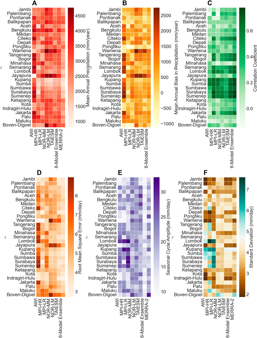
FIGURE 4. City-wise variation of different statistical metrics computed for precipitation across 29 cities in Indonesia (A) MA, (B) MBE, (C) CC, (D) RMSE, (E) SA, and (F) SD.

MBE for mean annual precipitation fluctuates from −1,000–2,500 mm/year. A correlation-based analysis was conducted for the monthly averaged precipitation data derived from the GCMs, 6ME, and MERRA-2 datasets from 1980 to 2014. Figure 4C demonstrates the city-specific CC. Subsequently, the values of the CC vary between −0.14 and 0.77.

An analysis associated with CC indicates that the 6ME performed exceptionally well across 22 cities. Figure 4D displays the RMSE range computed for mean monthly precipitation, ranging from 3 to 8 mm/day. Among the various GCMs, the 6ME exhibits the lowermost RMSE across all 21 cities, outperforming other models like TaiESM (MPI-HR) and AWI, demonstrating the smallest RMSE values for 3 and 2 cities, respectively.

In the case of precipitation, the SA ranges between 10 and 30 mm/day are depicted for each city (Figure 4E). Figure 4E depicts that for SA, NorMM demonstrated the best performance over seven cities, followed by the MPI-HR (6 cities) and AWI (5 cities). Across all the cities, the SD estimated from all the sources lies between 2 and 7 mm/day (Figure 4F). Subsequently, the trend of the SD obtained from both TaiESM and the 6ME closely resembles the actual SD trend observed in the reanalysis datasets.

4.1.3 Relative humidity

Figure 5A indicates the MA relative humidity. Across 29 cities, the average annual relative humidity estimated from all sources ranges from 70% to 92%. The MA relative humidity, resulting from six GCMs, including the 6ME, exhibits a stronger association with the MA relative humidity derived from MERRA-2 data.

FIGURE 5

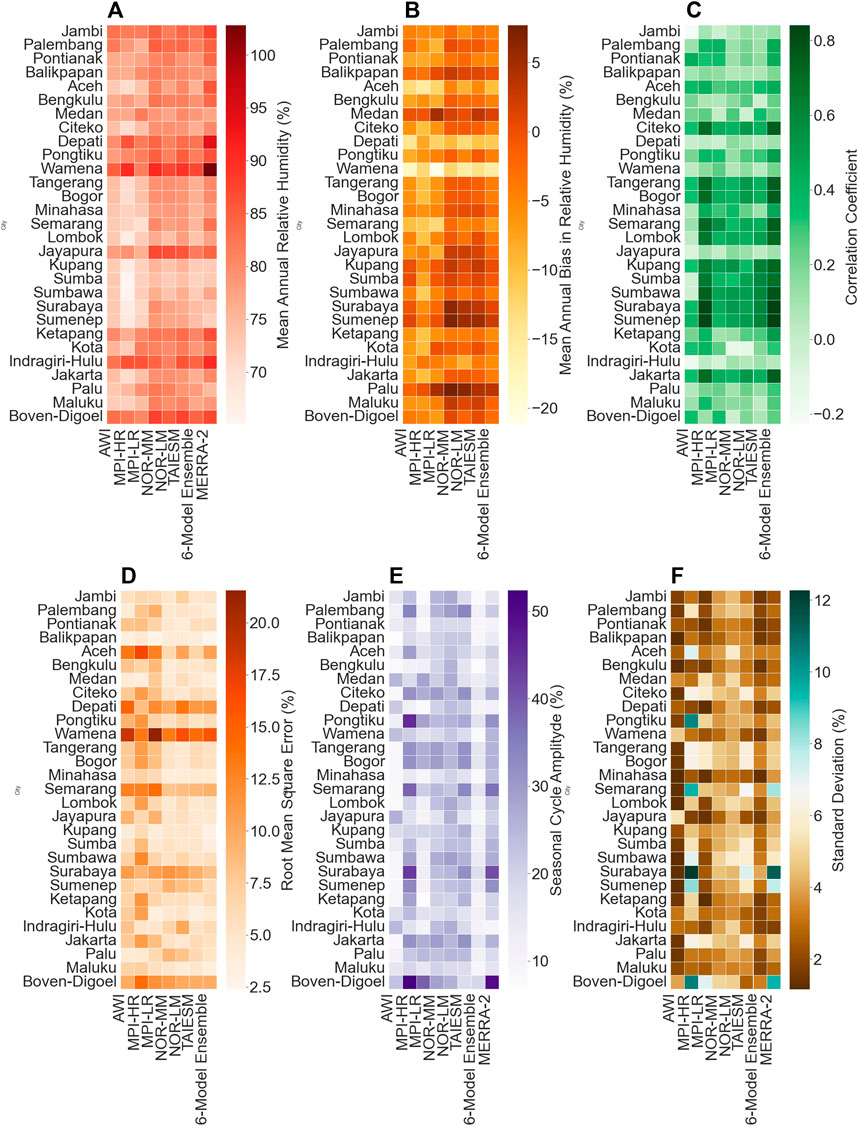
FIGURE 5. City-wise variation of different statistical metrics computed for relative humidity across 29 cities in Indonesia (A) MA, (B) MBE, (C) CC, (D) RMSE, (E) SA, and (F) SD.

Figure 5B illustrates the MBE in average annual relative humidity fluctuates between −21.58% and 7.69%. For each city, Figure 5C represents the outcomes of the correlation analysis conducted between the simulated and MERRA-2 datasets of monthly relative humidity. It shows that the CC varies from −0.22 to 0.84. Based on the correlation analysis, the 6ME was identified as the best performer for 19 cities.

Figures 5D, E represent the values of RMSE and SA, respectively. The RMSE breadth is from 3.52% to 21.54%, while the SA varies from 6% to 52.37%.

Figure 5F depicts the city-wise tendencies in the SD estimated from all the data sources. Among all the GCMs, The SD produced by NorMM, NorLM, and MPI-HR was found to be appropriate for six cities each.

4.1.4 Wind speed

Figure 6A demonstrates the variation in MA wind speed calculated using multiple GCMs, 6-ME, and a reanalysis dataset. For 29 cities, it varies from 0.44 m/s to 6.66 m/s. Figure 6B represents the MBE associated with the MA wind speed derived from 6ME and GCMs fluctuating between −1.25 m/s to 4.98 m/s. Figure 6C provides the outcomes of correlation analysis—further, the values of CC range from −0.38 to 0.72. Analysis of the CC indicates that among all cities, the performance of the 6ME was superior to 16 cities, followed by the MPI-HR, which was found to be suitable over seven cities. Figure 6D shows the city-wise alterations in the RMSE. The RMSE values span between 0.26 m/s to 5.22 m/s. Based on the RMSE, MPI-HR was the performing GCM over 14 major cities in Indonesia. The fluctuations in seasonal cycle amplitude of the mean monthly wind speed data are presented in Figure 6E. Considering the SA, the performance of AWI is exceptionally well over the five cities, whereas 6ME was found to be unfit for any location. In the case of SD, for all the cities, values vary from 0.08 m/s to 2.07 m/s (Figure 6F). Further, it has been observed that all the GCMs replicate the city-wise trend of standard deviation derived from the MERRA-2 dataset.

FIGURE 6

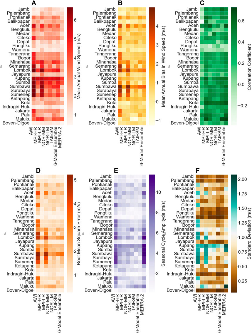
FIGURE 6. City-wise variation of different statistical metrics computed for for wind speed over 29 different cities of Indonesia during 1980–2014 (A) MA, (B) MBE, (C) CC, (D) RMSE, (E) SA, and (F) SD.

4.2 Total relative error

Across 29 cities, the total relative error was calculated for four meteorological parameters. It was calculated using the AHP method with different statistical measures. To obtain the weights for different statistical measures, an online survey was conducted in which more than four expert member opinions were considered through a survey sheet. Detailed information about the survey outline can be found in Supplementary Material S1. The survey outcomes are depicted in Table 5 with a CR value of 0.071. According to expert opinions, the RMSE and CC are the most important, followed by bias SD, bias in SA, and MBE, which are the least important. The total relative error is computed using the weights. The total relative error measures the closeness of simulated data to the reanalysis data. The total relative error values near zero indicate the good performance of the GCMs. For surface air temperature, the total relative error values for all the GCMs, including the 6ME, vary between 0.1 and 0.8 across 29 major cities of Indonesia (Figure 7A).

TABLE 5

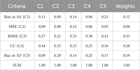
TABLE 5. Normalized matrix with the corresponding weights of each criterion for the total relative error. The λ_max and CI values are 5.32 and 0.07949, respectively.

FIGURE 7

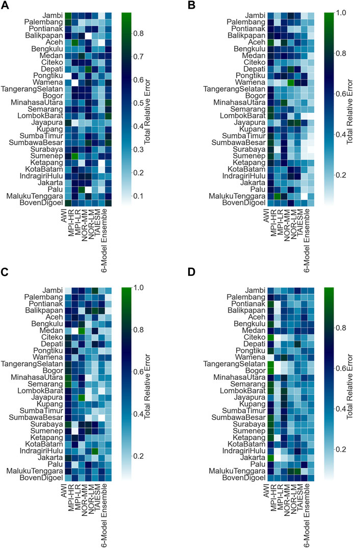
FIGURE 7. Total relative error depicting city-specific differences in the performance of each meteorological parameter (A) surface air temperature, (B) precipitation, (C) relative humidity, and (D) wind speed.

The simulated surface air temperature obtained from TaiESM was determined to have the lowest total relative error among 13 cities, making it the top-performing model. Following closely behind, the MPI-LR GCM exhibited superior performance over seven cities. In Wamena City, MPI-HR was identified as the model with the lowest total relative error (0.054) for surface air temperature.

On the contrary, NorMM exhibited the poorest performance, rendering it unsuitable for any individual city due to its unsatisfactory results. The city-wise total relative error for precipitation is shown in Figure 7B, and the 6ME performed exceptionally well for precipitation across 15 cities. The following 6ME, TaiESM, MPI-HR, and NorMM were found to be appropriate models for precipitation in 9, 4, and 1 city, respectively. However, the worst performers for precipitation were found to be AWI, MPI-LR, and NorLM.

The statistical evaluation of total relative error for relative humidity revealed that NorMM, MPI-HR, 6ME, TaiESM, AWI, and the NorLM demonstrated their suitability across 6, 6, 5, 5, 2, and 2 cities in Indonesia, respectively (Figure 7C).

Regarding wind speed, the analysis shows that MPI-HR is suitable for 19 cities and is the best-performing model. As shown in Figure 7D, NorLM and the 6ME were found to be adequate for 6 and 2 cities, respectively. In addition, regarding wind speed, AWI and TaiESM were found to be appropriate over the Wamena and Maluku Tenggara, respectively.

4.3 City-specific ranking

The generation of the future dataset of TMY is practically very complex, and it is tedious to downscale different meteorological parameters from different GCMs for a specific city, especially for non-climate scientists. Therefore, to identify the suitable city-specific GCM for future TMY generation, we have used the AHP method again by implementing the weighting factors associated with different meteorological variables, as shown in Table 6. According to expert opinion, the most important factors are temperature and relative humidity, followed by wind speed and precipitation. The weights of these weather variables will be used to calculate the appropriate GCMs in each city.

TABLE 6

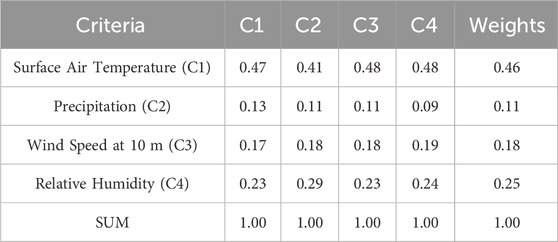
TABLE 6. Normalized matrix with the corresponding weights of each criterion for the meteorological variables. The λ_max, CI, and CR values are 4.01, 0.00389, and 0.004, respectively.

Figure 8 exhibits the city-wise optimal GCM for the generation of future TMY. The lower (higher) ranking score indicates the higher (lower) suitability of the GCM for generating future TMY data over specific cities. The city-specific ranking scores for each GCM range from 0.2 to 0.7. For all the cities, the ranking scores derived from AWI and MPI-LR range from 0.30 to 0.75, whereas ranking scores derived from other GCMs, including the 6ME, vary from 0.18 to 0.66. According to the city-specific ranking results, AWI is unsuitable for generating future TMY datasets for any city. These outcomes also reveal that among 29 cities, TaiESM (6ME) can be used over 18 (5) cities to generate the future TMY dataset. GCMs like MPI-LR, NorLM, and NorMM can be applied to cities such as Boven Digoel, Medan, and Bengkulu. Moreover, for generating future TMY data, MPI-HR was identified as appropriate for Wamena, Medan, and Depati cities. The list of GCMs that are appropriate for generating future TMY data specific to each city is given in Table 7.

FIGURE 8

FIGURE 8. City-specific ranking of the GCMs used for generating future TMY data.

TABLE 7

TABLE 7. List of optimal GCMs for generating the city-specific future TMY data.

5 Discussion

In the present study, the analysis of statistical measures for each meteorological variable, obtained by comparing the meteorological parameters derived from each GCM with reanalysis data, reveals a substantial variation in the performance of individual GCMs for each meteorological parameter. Notably, a GCM may exhibit strong performance for one statistical measure while showing weaker performance for another simultaneously. Therefore, expert judgment was used to allocate the distinct weights to each statistical measure estimated for each meteorological variable during the computation of the total relative error. Notably, more emphasis was placed on normalizing RMSE than any other statistical measure. A similar higher prominence on normalized RMSE was also corroborated by Srinivasa Raju and Nagesh Kumar, (2014) and Jose and Dwarakish, (2022).

The total relative error analysis demonstrates the city-specific performance of GCMs for various meteorological parameters (Figure 7D). Among all the GCMs, TaiESM, 6ME, NorMM/MPI-HR, and MPI-HR exhibit the best performance over a maximum number of cities in simulating the surface air temperature, precipitation, relative humidity, and wind speed, respectively. Additionally, our analysis associated with total relative error indicates that different GCMs’ performance varies with the cities and meteorological variables. Similar findings have been reported in prior studies, corroborating the outcomes of the total relative error (Firpo et al., 2022; Hemanandhini and Vignesh, 2023). Furthermore, the outcomes of total relative error, together with the results of the studies mentioned above, highlight that the performance of GCMs is inconsistent across cities or meteorological variables. This confirms that identifying city-specific, suitable GCMs will yield more precise and location-specific meteorological data. This, in turn, enables the generation of TMY datasets that can accurately reflect the variability in local climate.

To date, multiple authors have undertaken evaluations of the performance of CMIP6 G GCMs within the Indonesian and South Asian region context (Almazroui et al., 2020; Iqbal et al., 2021; Liu et al., 2023). These evaluations have primarily aimed to identify GCMs with high precision in simulating meteorological parameters. This collective effort has been instrumental in advancing our understanding of the capabilities and limitations of these models in capturing the complex meteorological patterns of Indonesia and other parts of the South Asian region.

While previous assessments have laid the groundwork by establishing the overall performance of GCMs, we have honed in on the practicality of these models by considering the varying levels of importance assigned to different cities within Indonesia. This approach allows us to identify GCMs that are accurate on a broader scale and tailored to the unique needs of specific cities. Subsequently, the present study takes a significant step forward by associating the importance of each meteorological parameter with the total relative error, pinpointing suitable GCMs for future TMY dataset generation based on city-specific needs.

The AHP methodology employed for GCM selection in forthcoming TMY data generation offers significant advantages:(i) It assesses the relative importance of each meteorological parameter during GCM selection for TMY data generation. (ii) the present approach also accounts for regional climate differences, reflecting the real-world variations in meteorological conditions across cities in Indonesia. This approach adds value to future climate modeling efforts by tailoring GCM selection to the specific needs of each location. (iii) The research contributes to the practical utility of the future TMY data generation process by streamlining the inclusion of necessary meteorological variables from the same GCM. This simplifies the dynamic downscaling process, making it more efficient and cost-effective.

6 Conclusion

This study utilized an AHP-based MCDA approach to identify a city-specific suitable GCM for generating future TMY datasets over 29 Indonesian cities. The evaluation process involved five statistical measures: correlation coefficient, root mean square error, mean bias error, standard deviation, and seasonal cycle amplitude. These metrics collectively assessed the model’s efficacy in-depth, providing a comprehensive understanding of its accuracy, bias, and capacity to capture crucial temporal variations. These statistical measures were calculated for surface air temperature, precipitation, relative humidity, and wind speed by comparing GCMs with reanalysis data. Different weights were assigned to the statistical measures based on expert opinions to determine the performance of each GCM in terms of total relative error. These weights were integrated to compute the city-specific performance of each GCM and every meteorological variable. The total relative error outcomes provided an understanding of the appropriate GCM for each meteorological parameter at each location. Next, the weights for individual meteorological parameters required to estimate TMY were calculated based on the expert’s opinion. Then, total relative errors were integrated to identify the city-specific suitable GCM for TMY generation, considering the respective weights. The major findings of this study are.

(i) GCM suitability outcomes derived for the individual meteorological variables and future TMY generation show that regionally best performing GCM need not be good at the city scale.

(ii) In terms of relative error estimated for individual meteorological variables indicate that among all the GCMs, TaiESM, 6Model-Ensemble, NorMM/MPI-HR, and MPI-HR exhibit the best performance over a maximum number of cities in simulating the surface air temperature, precipitation, relative humidity, and wind speed, respectively.

(iii) The evaluation of GCMs for the generation of the future TMY dataset shows that among 29 cities, TaiESM (6ME) can be used over 18 (5) cities to generate the future TMY dataset. GCMs like MPI-LR, NorLM, and NorMM can be applied to cities such as Boven Digoel, Medan, and Bengkulu. Moreover, for generating future TMY data, MPI-HR was identified as appropriate for Wamena, Medan, and Depati cities.

(iv) The assessment also shows TaiESM as a repeatedly suitable GCM for generating future TMY datasets across multiple cities. This finding suggests the model’s robustness and reliability in capturing the meteorological characteristics required for TMY generation.

(v) The AWI model was identified as the poorest-performing among all the GCMs, proving unsuitable for any of the cities under consideration.

This study did not comprehensively assess all potential aspects of CMIP6 GCM performance in simulating the climate of Indonesian cities. Instead, it focused on key climatic parameters essential for generating TMY data. Additionally, due to the unavailability of long-term ground observation data, the performance of all the GCMs was evaluated against reanalysis data in this study. Despite these limitations, the findings of this research present several advantages. Initially, it assists in identifying GCMs tailored to specific cities that excel in representing local meteorological conditions. This enables a focused allocation of resources for the most suitable GCMs, streamlining the downscaling process and enhancing efficiency. This targeted strategy reduces overall time and costs and contributes to a more precise and cost-effective future TMY generation. Secondly, the study enhances the production of accurate and reliable results by guiding the selection of GCMs closely aligned with the specific characteristics of the local climate. Thirdly, it optimizes resource allocation by directing researchers towards downscaling GCMs better suited to the intricacies of local conditions.

AHP is a promising method for identifying suitable GCM to generate future TMY datasets. However, it does have a limitation due to the subjectivity involved in choosing the weights of each meteorological variable based on expert judgments (Cabrera and Lee, 2020). Fortunately, this limitation can be addressed by the consistency ratio threshold specified by Saaty (1980). In this study, each response was carefully assessed. Responses with inconsistent results (i.e., the CR > 10%) were not included in the final evaluation, reducing the number of acceptable respondents. Having fewer respondents might not capture a broader perspective. While having many respondents in AHP is not strictly required, having more respondents can help capture a broader consensus. Nevertheless, by employing AHP, this research has provided valuable insights into selecting appropriate GCMs for making realistic projections of the future TMY under varying climate change scenarios.

In the future, employing recommended city-specific GCMs for generating future TMY datasets is critical for architectural researchers and policymakers worldwide. This practice enhances the accuracy of climate projections, offering valuable insights for informed urban planning and design decisions. Moreover, it facilitates the implementation of sustainable building practices and plays a pivotal role in shaping effective climate policies for the future. The approach tested in this study provides a universal method for selecting GCMs for preparing future TMY datasets, applicable across the globe for comprehensive climate modeling and planning.

Data availability statement

The original contributions presented in the study are included in the article/Supplementary Material, further inquiries can be directed to the corresponding author.

Author contributions

VB: Conceptualization, Data curation, Formal Analysis, Investigation, Methodology, Software, Validation, Visualization, Writing–original draft, Writing–review and editing. HL: Conceptualization, Formal Analysis, Supervision, Writing–original draft, Writing–review and editing. JC: Methodology, Writing–original draft. TK: Conceptualization, Project administration, Supervision, Writing–original draft. RP: Data curation, Investigation, Writing–original draft. FR: Data curation, Writing–original draft. HN: Supervision, Writing–original draft.

Funding

The author(s) declare that financial support was received for the research, authorship, and/or publication of this article. This research was conducted by the Climate Research Group for the Development of Standard Weather Data as part of the Development of Low-Carbon Affordable Apartments in the Hot-Humid Climate of Indonesia Project toward Paris Agreement 2030; the Science and Technology Research Partnership for Sustainable Development (SATREPS); and collaboratively supported by the Japan Science and Technology Agency (JST, JP-MJSA1904), the Japan International Cooperation Agency (JICA), Hiroshima University, Kagoshima University, the Ministry of Public Works and Housing (PUPR) of Indonesia, and the Meteorological, Climatological, and Geophysical Agency (BMKG) of Indonesia.

Conflict of interest

The authors declare that the research was conducted in the absence of any commercial or financial relationships that could be construed as a potential conflict of interest.

Publisher’s note

All claims expressed in this article are solely those of the authors and do not necessarily represent those of their affiliated organizations, or those of the publisher, the editors and the reviewers. Any product that may be evaluated in this article, or claim that may be made by its manufacturer, is not guaranteed or endorsed by the publisher.

Supplementary material

The Supplementary Material for this article can be found online at: https://www.frontiersin.org/articles/10.3389/fenvs.2024.1341807/full#supplementary-material

References

Alizadeh, O. (2022). Advances and challenges in climate modeling. Clim. Change 170, 18. doi:10.1007/s10584-021-03298-4

CrossRef Full Text | Google Scholar

Almazroui, M., Saeed, S., Saeed, F., Islam, M. N., and Ismail, M. (2020). Projections of precipitation and temperature over the South Asian countries in CMIP6. Earth Syst. Environ. 4, 297–320. doi:10.1007/s41748-020-00157-7

CrossRef Full Text | Google Scholar

Ambade, B., Sankar, T. K., Panicker, A. S., Gautam, A. S., and Gautam, S. (2021). Characterization, seasonal variation, source apportionment and health risk assessment of black carbon over an urban region of East India. Urban Clim. 38, 100896. doi:10.1016/j.uclim.2021.100896

CrossRef Full Text | Google Scholar

Arnell, N. W., Lowe, J. A., Bernie, D., Nicholls, R. J., Brown, S., Challinor, A. J., et al. (2019). The global and regional impacts of climate change under representative concentration pathway forcings and shared socioeconomic pathway socioeconomic scenarios. Environ. Res. Lett. 14, 084046. doi:10.1088/1748-9326/ab35a6

CrossRef Full Text | Google Scholar

Bhanage, V., Kulkarni, S., Sharma, R., Lee, H. S., and Gedam, S. (2023a). Enumerating and modelling the seasonal alterations of surface urban heat and cool island: a case study over Indian cities. Urban Sci. 7, 38. doi:10.3390/urbansci7020038

CrossRef Full Text | Google Scholar

Bhanage, V., Lee, H. S., Kubota, T., Pradana, R. P., Fajary, F. R., Arya Putra, I. D. G., et al. (2023b). City-wise assessment of suitable CMIP6 GCM in simulating different urban meteorological variables over major cities in Indonesia. Climate 11, 100. doi:10.3390/cli11050100

CrossRef Full Text | Google Scholar

Bosilovich, M. G. (2015). MERRA-2: initial evaluation of the climate. Greenbelt, MD, United States: National Aeronautics and Space Administration, Goddard Space Flight Center.

Google Scholar

Cabrera, J. S., and Lee, H. S. (2020). Flood risk assessment for Davao Oriental in the Philippines using geographic information system-based multi-criteria analysis and the maximum entropy model. J. Flood Risk Manag. 13, 1–17. doi:10.1111/jfr3.12607

CrossRef Full Text | Google Scholar

Cebecauer, T., and Suri, M. (2015). Typical meteorological year data: SolarGIS approach. Energy Procedia 69, 1958–1969. doi:10.1016/j.egypro.2015.03.195

CrossRef Full Text | Google Scholar

Chowdhury, P., and Behera, M. R. (2019). Evaluation of CMIP5 and CORDEX derived wave climate in Indian Ocean. Clim. Dyn. 52, 4463–4482. doi:10.1007/s00382-018-4391-0

CrossRef Full Text | Google Scholar

Dias, J. B., da Graca, G. C., and Soares, P. M. M. (2020). Comparison of methodologies for generation of future weather data for building thermal energy simulation. Energy Build. 206, 109556. doi:10.1016/j.enbuild.2019.109556

CrossRef Full Text | Google Scholar

Doocy, S., Daniels, A., Dooling, S., and Gorokhovich, Y. (2013). The human impact of volcanoes: a historical review of events 1900-2009 and systematic literature review. PLoS Curr. 5. doi:10.1371/currents.dis.841859091a706efebf8a30f4ed7a1901

PubMed Abstract | CrossRef Full Text | Google Scholar

Eyring, V., Bony, S., Meehl, G. A., Senior, C. A., Stevens, B., Stouffer, R. J., et al. (2016). Overview of the coupled model intercomparison project phase 6 (CMIP6) experimental design and organization. Geosci. Model Dev. 9, 1937–1958. doi:10.5194/gmd-9-1937-2016

CrossRef Full Text | Google Scholar

Field, C. B. (2014). Climate change 2014: impacts, adaptation and vulnerability: working Group II contribution to the fifth assessment report of the intergovernmental panel on climate change. Cambridge, United Kingdom: Cambridge University Press.

Google Scholar

Fildes, R., and Kourentzes, N. (2011). Validation and forecasting accuracy in models of climate change. Int. J. Forecast. 27, 968–995. doi:10.1016/j.ijforecast.2011.03.008

CrossRef Full Text | Google Scholar

Firpo, M. A. F., Guimarães, B., Dantas, L. G., Silva, M. G. B. da, Alves, L. M., Chadwick, R., et al. (2022). Assessment of CMIP6 models’ performance in simulating present day climate in Brazil. Front. Clim. 170. doi:10.3389/fclim.2022.948499

CrossRef Full Text | Google Scholar

Gautam, S., Sammuel, C., Bhardwaj, A., Shams Esfandabadi, Z., Santosh, M., Gautam, A. S., et al. (2021). Vertical profiling of atmospheric air pollutants in rural India: a case study on particulate matter (PM10/PM2.5/PM1), carbon dioxide, and formaldehyde. Meas. J. Int. Meas. Confed. 185, 110061. doi:10.1016/j.measurement.2021.110061

CrossRef Full Text | Google Scholar

Gidden, M. J., Riahi, K., Smith, S. J., Fujimori, S., Luderer, G., Kriegler, E., et al. (2019). Global emissions pathways under different socioeconomic scenarios for use in CMIP6: a dataset of harmonized emissions trajectories through the end of the century. Geosci. Model Dev. 12, 1443–1475. doi:10.5194/gmd-12-1443-2019

CrossRef Full Text | Google Scholar

Gleick, P. H. (1986). Methods for evaluating the regional hydrologic impacts of global climatic changes. J. Hydrol. 88, 97–116. doi:10.1016/0022-1694(86)90199-x

CrossRef Full Text | Google Scholar

Haase, M., Andresen, I., and Hestnes, A. G. (2011). The development of future weather data files for Norway. Int. J. Clim. Chang. Impacts Responses 2, 1–24. doi:10.18848/1835-7156/cgp/v02i03/37327

CrossRef Full Text | Google Scholar

Hemanandhini, S., and Vignesh, R. L. (2023). Performance evaluation of CMIP6 climate models for selecting a suitable GCM for future precipitation at different places of Tamil Nadu. Environ. Monit. Assess. 195, 928. doi:10.1007/s10661-023-11454-9

PubMed Abstract | CrossRef Full Text | Google Scholar

Huld, T., Paietta, E., Zangheri, P., and Pinedo Pascua, I. (2018). Assembling typical meteorological year data sets for building energy performance using reanalysis and satellite-based data. Atmos. (Basel) 9, 53. doi:10.3390/atmos9020053

CrossRef Full Text | Google Scholar

Iqbal, Z., Shahid, S., Ahmed, K., Ismail, T., Ziarh, G. F., Chung, E.-S., et al. (2021). Evaluation of CMIP6 GCM rainfall in mainland Southeast asia. Atmos. Res. 254, 105525. doi:10.1016/j.atmosres.2021.105525

CrossRef Full Text | Google Scholar

Jose, D. M., and Dwarakish, G. S. (2022). Ranking of downscaled CMIP5 and CMIP6 GCMs at a basin scale: case study of a tropical river basin on the South West coast of India. Arab. J. Geosci. 15, 120–123. doi:10.1007/s12517-021-09289-0

CrossRef Full Text | Google Scholar

Kurniadi, A., Weller, E., Kim, Y.-H., and Min, S.-K. (2023). Evaluation of coupled model intercomparison project phase 6 model-simulated extreme precipitation over Indonesia. Int. J. Climatol. 43, 174–196. doi:10.1002/joc.7744

CrossRef Full Text | Google Scholar

Li, H., Huang, J., Hu, Y., Wang, S., Liu, J., and Yang, L. (2021). A new TMY generation method based on the entropy-based TOPSIS theory for different climatic zones in China. Energy 231, 120723. doi:10.1016/j.energy.2021.120723

CrossRef Full Text | Google Scholar

Liu, S., Raghavan, S. V., Ona, B. J., and Nguyen, N. S. (2023). Bias evaluation in rainfall over Southeast Asia in CMIP6 models. J. Hydrol. 621, 129593. doi:10.1016/j.jhydrol.2023.129593

CrossRef Full Text | Google Scholar

McSweeney, C. F., Jones, R. G., Lee, R. W., and Rowell, D. P. (2015). Selecting CMIP5 GCMs for downscaling over multiple regions. Clim. Dyn. 44, 3237–3260. doi:10.1007/s00382-014-2418-8

CrossRef Full Text | Google Scholar

Nik, V. M. (2016). Making energy simulation easier for future climate–Synthesizing typical and extreme weather data sets out of regional climate models (RCMs). Appl. Energy 177, 204–226. doi:10.1016/j.apenergy.2016.05.107

CrossRef Full Text | Google Scholar

Pimonsree, S., Kamworapan, S., Gheewala, S. H., Thongbhakdi, A., and Prueksakorn, K. (2023). Evaluation of CMIP6 GCMs performance to simulate precipitation over Southeast Asia. Atmos. Res. 282, 106522. doi:10.1016/j.atmosres.2022.106522

CrossRef Full Text | Google Scholar

Rahman, A., and Pekkat, S. (2024). Identifying and ranking of CMIP6 - global climate models for projected changes in temperature over Indian subcontinent. Sci. Rep. 14, 3076–3114. doi:10.1038/s41598-024-52275-1

PubMed Abstract | CrossRef Full Text | Google Scholar

Rivera, P. (2023). Climate change projections in Guatemala: temperature and precipitation changes according to CMIP6 models. Model. Earth Syst. Environ., 1–19. doi:10.1007/s40808-023-01881-5

CrossRef Full Text | Google Scholar

Ruane, A. C., and McDermid, S. P. (2017). Selection of a representative subset of global climate models that captures the profile of regional changes for integrated climate impacts assessment. Earth Perspect. 4, 1–20. doi:10.1186/s40322-017-0036-4

CrossRef Full Text | Google Scholar

Saaty, T. L. (1980). The analytical hierarchy process, planning, priority. USA: Resour. Alloc. RWS Publ.,

Google Scholar

Santamouris, M. (2016). Cooling the buildings–past, present and future. Energy Build. 128, 617–638. doi:10.1016/j.enbuild.2016.07.034

CrossRef Full Text | Google Scholar

Shiru, M. S., and Chung, E.-S. (2021). Performance evaluation of CMIP6 global climate models for selecting models for climate projection over Nigeria. Theor. Appl. Climatol. 146, 599–615. doi:10.1007/s00704-021-03746-2

CrossRef Full Text | Google Scholar

Srinivasa Raju, K., and Nagesh Kumar, D. (2014). Ranking general circulation models for India using TOPSIS. J. Water Clim. Chang. 6, 288–299. doi:10.2166/wcc.2014.074

CrossRef Full Text | Google Scholar

Stocker, T. (2014). Climate change 2013: the physical science basis: working Group I contribution to the fifth assessment report of the intergovernmental panel on climate change. Cambridge, United Kingdom: Cambridge University Press.

Google Scholar

Teske, S., Pregger, T., Simon, S., Naegler, T., Pagenkopf, J., Deniz, Ö., et al. (2021). It is still possible to achieve the paris climate agreement: regional, sectoral, and land-use pathways. Energies 14, 2103. doi:10.3390/en14082103

CrossRef Full Text | Google Scholar

Thapliyal, J., Bhattacharyya, M., Prakash, S., Patni, B., Gautam, S., and Gautam, A. S. (2022). Addressing the relevance of COVID–19 pandemic in nature and human socio-economic fate. Stoch. Environ. Res. Risk Assess. 36, 3239–3253. doi:10.1007/s00477-022-02191-5

PubMed Abstract | CrossRef Full Text | Google Scholar

Troup, L., Eckelman, M. J., and Fannon, D. (2019). Simulating future energy consumption in office buildings using an ensemble of morphed climate data. Appl. Energy 255, 113821. doi:10.1016/j.apenergy.2019.113821

CrossRef Full Text | Google Scholar

Vinayak, B., Lee, H. S., Gedam, S., and Latha, R. (2022). Impacts of future urbanization on urban microclimate and thermal comfort over the Mumbai metropolitan region, India. Sustain. Cities Soc. 79, 103703. doi:10.1016/j.scs.2022.103703

CrossRef Full Text | Google Scholar

Vinayak, B., Lee, H. S., and Gedem, S. (2021). Prediction of land use and land cover changes in Mumbai city, India, using remote sensing data and a multilayer perceptron neural network-based Markov chain model. Sustain 13, 471. doi:10.3390/su13020471

CrossRef Full Text | Google Scholar

Vr, L. (2023). Performance evaluation of CMIP6 climate models for selecting a suitable GCM for future precipitation at different places of Tamil Nadu. Environ. Monit. Assess. 195, 928. doi:10.1007/s10661-023-11454-9

PubMed Abstract | CrossRef Full Text | Google Scholar

Yuan, J., Huang, P., and Chai, J. (2022). Development of a calibrated typical meteorological year weather file in system design of zero-energy building for performance improvements. Energy 259, 125031. doi:10.1016/j.energy.2022.125031

CrossRef Full Text | Google Scholar

Zhang, X., Alexander, L., Hegerl, G. C., Jones, P., Tank, A. K., Peterson, T. C., et al. (2011). Indices for monitoring changes in extremes based on daily temperature and precipitation data. Wiley Interdiscip. Rev. Clim. Chang. 2, 851–870. doi:10.1002/wcc.147

CrossRef Full Text | Google Scholar