 Brian Timmer
 Luba Y. Reshitnyk
 Margot Hessing-Lewis
 Francis Juanes
 Lianna Gendall
 Maycira Costa
- 1Spectral Lab, Department of Geography, University of Victoria, Victoria, BC, Canada
- 2Hakai Institute, Heriot Bay, BC, Canada
- 3Department of Biology, University of Victoria, Victoria, BC, Canada
Surface-canopy forming kelps (Macrocystis pyrifera and Nereocystis luetkeana) can be monitored along the Northeast Pacific coast using remote sensing. These kelp canopies can be submerged by tides and currents, making it difficult to accurately determine their extent with remote sensing techniques. Further, both species have morphologically distinct canopies, each made up of structures with differing buoyancies, and it is not well understood whether the differing buoyancies between these species’ canopies affects their detectability with remote sensing technologies. Here, we collected in situ above-water spectral signatures for the surface-canopies of Nereocystis and Macrocystis, providing the first direct hyperspectral comparison between the structures that make up the canopies of these species. Additionally, we compare the strength of their red-edge and near-infrared band signals, as well as the normalized difference red-edge (NDRE) and normalized difference vegetation index (NDVI) values. At the bed level, we compare detection of kelp canopy extent using both NDRE and NDVI classified unoccupied aerial vehicle imagery. We also characterized how changing tides and currents submerge the canopies of both species, providing insights that will allow remote sensors to more accurately determine the extent of kelp canopy in remote sensing imagery. Observations of canopy structures paired with in situ hyperspectral data and simulated multispectral data showed that more buoyant kelp structures had higher reflectance in the near-infrared wavelengths, but even slightly submerged canopy structures had a higher reflectance in the red-edge rather than the near-infrared. The higher red-edge signal was also evident at the bed level in the UAV imagery, resulting in 18.0% more canopy classified with NDRE than with NDVI. The area of detected canopy extent decreased by an average of 22.5% per meter of tidal increase at low current speeds (<10 cm/s), regardless of the species present. However, at higher current speeds (up to 19 cm/s), Nereocystis canopy decreased at nearly twice the average rate of kelp beds in low-current conditions. Apart from the strong differences in high-current regions, a robust linear relationship exists between kelp canopy extent and tidal height, which can aid in understanding the errors associated with remote sensing imagery collected at different tidal heights.
1 Introduction
Kelp forests are highly productive marine ecosystems that provide numerous ecologically and commercially important ecosystem services (Mann, 1973; Krumhansl and Scheibling, 2012). In the Northeast Pacific, Macrocystis pyrifera (giant kelp) and Nereocystis luetkeana (bull kelp) are two important kelp species that form morphologically distinct floating surface-canopies, both of which can be monitored using remote sensing methodologies (Pfister et al., 2017; Nijland et al., 2019; Cavanaugh et al., 2021a; Gendall et al., 2023). The presence and area of surface-canopy can be highly variable for both of these species, both spatially and temporally, according to numerous environmental factors. In recent decades, some kelp forests have undergone significant reductions in extent or even extirpation, making it important to monitor changes in these vital ecosystems (Krumhansl et al., 2016; Wernberg et al., 2019; Starko et al., 2022). Measuring temporal changes to the canopy extent of these kelps from aerial and satellite imagery is essential to effectively understand how environmental drivers, such as inter-annual and decadal climate regimes (Pfister et al., 2017; Schroeder et al., 2019a; Bell et al., 2020a; Gendall et al., 2023), or how pulse events like marine heatwaves (Arafeh-Dalmau et al., 2019; Starko et al., 2022) influence the spatial and temporal persistence of kelp forests.
Remote sensing is an effective technology used to monitor floating kelp at both local and regional scales (e.g., Schroeder et al., 2019a; Cavanaugh et al., 2021a; Gendall et al., 2023). The remote sensing of floating kelp canopy relies on the kelp’s high reflectance in the near-infrared (NIR) (700–1,000 nm) in contrast with the surrounding water’s low NIR reflectance (Jensen, 1980; Schroeder et al., 2019b; Timmer et al., 2022). However, in situ oceanographic and biological conditions during remote sensing imagery acquisition can introduce uncertainties when measuring kelp extent. For example, portions of the kelp canopy may be submerged by changing tides and associated tidal currents (Britton-Simmons et al., 2008; Cavanaugh et al., 2021b), or simply due to the morphological differences in the canopies and their position at the water’s surface (Schroeder et al., 2019b). Further, different parts of the kelp canopy (e.g., Nereocystis pneumatocyst vs blades) are either positively or negatively buoyant, which can lead to a spectral signal containing both submerged kelp (low NIR reflectance) and floating kelp (high NIR reflectance) with the surrounding water (Schroeder et al., 2019b; Timmer et al., 2022). The above-water reflectance of both floating and submerged kelp detected with remote sensing is a combination of the kelp and water’s spectral signals, which are further influenced by the presence of optically active water components (e.g., chlorophyll or suspended sediments) (Mobley, 1994).
Specifically, when kelp is submerged, the typically high NIR signal is dampened by the water molecules’ strong absorption, potentially reducing the detectability of submerged canopy with an above-water sensor (Augenstein et al., 1991; Schroeder et al., 2019b; Cavanaugh et al., 2021b; Timmer et al., 2022). Generally, this problem can be minimized by collecting remote sensing imagery at relatively low tidal heights and during times when current speeds are relatively low, when most kelp canopy is expected to be floating at or near the water’s surface (Pfister et al., 2017; Schroeder et al., 2019a; Nijland et al., 2019; Hamilton et al., 2020). However, tidal ranges can vary substantially across regions, making both the planning of imagery acquisition and the selection of archived imagery during low tides and under cloud-free conditions (where kelp can be seen), challenging. For example, moving northward from California toward Alaska, the tidal range and frequency of cloud cover both generally increase, limiting the availability of cloud-free, low-tide imagery (Cavanaugh et al., 2021a). Further, nearshore currents can be highly heterogeneous over space and time, often decoupling completely from open water currents in straits or channels where current speeds are often the fastest (Britton-Simmons et al., 2008), making it difficult to predict the effects of currents on kelp detection within remote sensing imagery, even when tidal height and cloud cover are ideal.
Given these constraints, remote sensing imagery for mapping kelp on the Northeast Pacific Coast have been acquired within a range of conditions, with potentially significant implications on the accuracy of the mapped kelp canopy extent (Schroeder et al., 2019a; Nijland et al., 2019; Gendall et al., 2023). Recently, narrow-band multispectral UAV imagery has been used to measure the effects of tides and currents on Macrocystis beds in California (Cavanaugh et al., 2021b), allowing analyses at high spatial (centimeters) and temporal (minutes) resolutions that are not currently possible with satellite imagery (sub-meter to meters; days to weeks) (Nijland et al., 2019; Mora-Soto et al., 2020). Similar UAV comparisons have not been conducted for Macrocystis kelp forests in British Columbia, where both tidal ranges and current variability are higher, nor have UAV comparisons been conducted for Nereocystis in any region.
Beyond the uncertainties associated with in situ oceanographic and biological conditions, sensor characteristics may also influence kelp detection. These characteristics include the different spectral bands or wavelengths available for kelp classification (Augenstein et al., 1991; Schroeder et al., 2019b; Cavanaugh et al., 2021b). For instance, light absorption by water and its optical constituents is generally the lowest in the visible wavelengths and increases exponentially at longer wavelengths. As such, wavelengths in the longer NIR ranges (e.g., >800 nm) are subject to higher absorption than the shorter wavelengths in the red-edge (RE) range (670–750 nm) (Mobley, 1994). As a result, the RE wavelengths can penetrate deeper into the water column, allowing for deeper kelp canopy detection than possible with longer NIR wavelengths (see Timmer et al., 2022 for detailed discussion of this phenomenon) and higher separability between the classes of kelp and water during imagery classification (Mora-Soto et al., 2020; Cavanaugh et al., 2021b). However, some of the first-generation satellite sensors (e.g., Landsat and SPOT series) have been used to map historical kelp based on the NIR band, but were not designed to measure reflectance at RE wavelengths (Tucker, 1978; Barsi et al., 2014; Schroeder et al., 2019b). As such, long-term remote sensing studies generally focus on the NIR bands for kelp classification, often either using the normalized difference vegetation index (NDVI) to enhance and standardize kelp detection, or using an NIR band directly as part of Multiple Endmember Spectral Mixture Analysis (MESMA) (Jensen, 1980; Schroeder et al., 2019b; Nijland et al., 2019; Bell et al., 2020a; Butler et al., 2020; Hamilton et al., 2020; Gendall et al., 2023). Given the many potential uncertainties when using remote sensing to monitor kelp, it is critical to understand how morphological differences in their canopy structures and the resulting differences in their buoyancy can affect different regions of the kelp spectral reflectance. Further, a better understanding of how these kelps are submerged by tides and currents and whether certain spectral bands or vegetation indices can be used to enhance the detection of their submerged structures is also critical for using remote sensing for kelp mapping.
In this study, our goals were two-fold: (1) to describe spectral characteristics that arise from morphological and bed-level differences between Macrocystis and Nereocystis surface-canopies, and (2) to quantify the effects of local tides and currents on the apparent canopy extent for both Macrocystis and Nereocystis using remote sensing imagery. To address these goals, (i) we characterized the spectral differences between Nereocystis and Macrocystis canopy structures using both in situ hyperspectral and simulated multispectral measurements, as well as multispectral UAV imagery, and (ii) we investigated the relationship between the canopy extents of both Nereocystis and Macrocystis derived from multispectral UAV imagery with associated tidal height and current speed. This work contributes to global efforts to monitor surface-canopy forming kelps by detailing the first direct comparison of the in situ above-water spectral signatures of Nereocystis and Macrocystis canopy structures. It also adds to the limited scientific knowledge of how both species’ canopy structures respond to submergence by tides and tidal currents. Together, this information empirically assesses the variability and uncertainty in remote sensing of kelp extent, allowing remote sensors to make informed decisions to increase the accuracy of mapped kelp.
2 Materials and methods
2.1 Study site selection and characterization
This research was conducted at six sites located near the Hakai Institute ecological observatory on Calvert Island (51°39′16″N 128°07′53″W) on the Central Coast of British Columbia over 2 weeks in July 2020 (Figure 1). The region is characterized by a complex coastline with numerous channels, fjords, and islands, creating a mosaic of habitats for aquatic vegetation (Nijland et al., 2019; Olson et al., 2019). Mean sea surface temperatures range from 7°C to 15°C annually (Jackson et al., 2015), and tides in the region are semi-diurnal, with tidal exchanges ranging between 3 and 5 m (Thomson, 1981). The two dominant surface-canopy forming kelp species are M. pyrifera and N. luetkeana, which can be found in mono-specific and/or mixed beds (Sutherland, 2008; Nijland et al., 2019). Both species are generally found between zero to 10 m below chart datum on the BC coast, but are most commonly found at less than 5 m depth [McHenry et al., 2024 (under review)]. Although species-level abundance data are uncommon for this region, aerial surveys conducted by the government of British Columbia show that between 1993 and 2007, a significant shift occurred from Nereocystis to Macrocystis-dominated reefs (Sutherland, 2008). Since then, changes in kelp abundance have occurred locally at different sites, likely as a result of trophic cascades (Burt et al., 2018) and climatic shifts (Krumhansl et al., 2016).
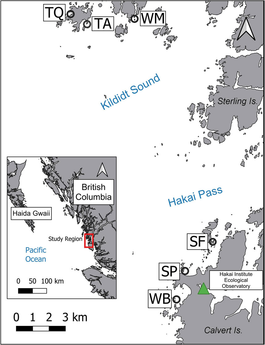
FIGURE 1. Survey site locations on the Central Coast of British Columbia. Site names are based on The Hakai Institute’s existing kelp monitoring program. TQ = Triquet Bay (one Macrocystis bed), TA = Triquetta (two Nereocystis beds), WM = Womanley (one Macrocystis bed), SF = Starfish Channel (one Macrocystis bed and one Nereocystis bed), SP = Surf Pass (one mixed bed), WB = Westbeach (one Macrocystis bed).
To account for environmental variability of kelp beds along the heterogeneous coastline, a range of site types were surveyed (e.g., bays, channels, headlands) across various conditions (e.g., exposure, current speeds) that included both Macrocystis and Nereocystis beds, with site selection based on expert knowledge from the Hakai Institute’s kelp monitoring program (https://hakai.org/). Within these sites, the bathymetric extent of all kelp beds was between 0 and −5 m based on the lower low water large tide (LLWLT) chart datum. Study site selection required: (1) distinct kelp beds that a UAV could collect imagery of within a single flight, (2) relatively flat subtidal benthos near the kelp bed for the benthic placement of an acoustic Doppler current profiler (ADCP) to collect concurrent tide and current data; (3) a nearby shoreline that could be captured in imagery and used for georeferencing UAV images; and (4) deep enough bathymetry so the canopy did not mix with lower intertidal or upper subtidal species (e.g., surf-grass or understory kelps) at the lowest tides. Two sites (Triquetta and Starfish) contained two distinct kelp beds each within the UAV flight path (Figure 1). Therefore, a total of eight beds were analyzed even though only six sites were surveyed: four Macrocystis, three Nereocystis, and one mixed bed with both species present (Table 1).
TABLE 1. List of bed codes used for each kelp bed surveyed, according to site and species present. Note that bed codes are simply site codes from Figure 1, but with suffixes added to distinguish when two beds are located at the same site.
2.2 Kelp morphological characteristics: implications for remote sensing detection
Macrocystis and Nereocystis kelp canopies are morphologically distinct from one another, and the buoyancy of their canopies is directly related to the canopy morphology (Burnett and Koehl, 2017). The strength of a kelp canopy reflectance signal, as detected by an above-water sensor, will vary based on the buoyancy of the canopy and its emergence at the water’s surface (Timmer et al., 2022). From a strictly remote sensing perspective, here we consider three distinct kelp canopy “structure types”: The Nereocystis pneumatocyst, the Nereocystis blades, and the Macrocystis fronds. The Nereocystis pneumatocyst is a single elongated gas bladder, often many meters long, that transitions into a stipe and is anchored to the benthos by a holdfast. Up to 60 blades, which are often around 4 m long, trail from the distal end of the Nereocystis pneumatocyst (Springer et al., 2007; Koehl et al., 2008) and are usually held aloft just below the surface in the water column by passing currents (Koehl et al., 2008). When mapping Nereocystis with a UAV the pneumatocyst and blades of Nereocystis sit differently at the water’s surface due to their positive and negative buoyancy, and are readily distinguishable from one another (Figure 2). In comparison, the Macrocystis canopy is comprised of multiple smaller structures that are not generally individually distinguishable, even in high resolution UAV imagery (Figure 2). This collection of Macrocystis canopy structures is commonly referred to as fronds. A Macrocystis frond is made up of numerous thin stipes rising from a large holdfast on the sea floor, with each stipe lined with many small buoyant pneumatocysts and a single negatively buoyant blade protruding from the distal end of each pneumatocyst (Druehl and Wheeler, 1986). The combined buoyancy of the many small pneumatocysts holds the fronds at the surface, but portions of the frond (e.g., the blades) may still sit largely just below the water’s surface. With increasing interest in using ultra high-resolution remote sensing imagery to understand metrics like kelp biomass and health (Bell et al., 2020b), we believe that it is useful to better understand the remote sensing implications of these unique kelp canopy “structure types” and their morphological differences.
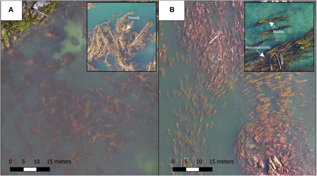
FIGURE 2. Unoccupied aerial vehicle imagery collected at 90 m altitude showing a nadir view of the morphological distinction between (A) Macrocystis pyrifera fronds, along with higher resolution inset where the bulbs, blades, and stipe cannot be as easily distinguished from one another; as well as (B) Nereocystis luetkeana with pneumatocysts prominent at the surface near rocks and blades prominent near the surface in the channel between the rocks, along with higher resolution inset showing these same features.
2.3 Data collection and processing
2.3.1 Biophysical water properties and in situ above-water reflectance
Water optical properties can be highly variable along the coast of British Columbia due to contributions from glacial fjords and estuaries, characterized by high sediment loads, which significantly increase the reflectance across all wavelengths between the red and the NIR regions of water spectra (Loos and Costa, 2010; Phillips and Costa, 2017; Giannini et al., 2021). In addition, intense phytoplankton blooms can increase reflectance in the NIR region of water spectra, especially at the RE wavelengths (Schalles et al., 1998). The variable concentrations of these optical water constituints may bias classification results by obscuring spectral features used to detect aquatic vegetation (Dekker et al., 2005; O’Neill and Costa, 2013; Murray et al., 2015). To account for the possible changes in water optical constituents during the field survey, water quality measurements were conducted at each site, including under-water hyperspectral downwelling irradiance from a Satlantic Hyperpro profiler that was lowered through the water column with a boat-mounted downrigger. The profiler acquired down-welling irradiance at a 2-nm spectral resolution with a spectral range of 300–800nm, every 0.1 m depth. These data were used to calculate the diffuse attenuation coefficient (Kd) (a proxy for light penetration in the water column) between 400 and 800 nm within the top 1 m of the water column, using Satlantic software and following the methods outlined by O’Neill et al. (2011). Further details about the calculation of Kd can be found in Supplementary Material S1. Water samples were collected in triplicate to determine total suspended matter (TSM), percent organic matter (POM) and percent inorganic matter (PIM) (Phillips and Costa, 2017). Finally, Secchi depth was collected at each site as a proxy for water clarity (Gallegos et al., 2011). Together with the above-water spectra, the Kd, TSM, POM, PIM, and Secchi depth data informed the range and variability of water conditions during field data acquisition.
To characterize the in situ spectral differences between kelp canopy ‘structure types’, above-water spectra were collected for dense samples of each structure (i.e., the field of view containing ∼100% spectral target - either Macrocystis fronds, Nereocystis pneumatocysts, or Nereocystis blades) using an ASD Fieldspec Handheld 2 spectroradiometer (325–1,075 nm) aboard a 22′ aluminum motor vessel following target acquisition methods by (O’Neill et al., 2011). Above-water spectra were also collected over optically deep water to supplement the water quality measurements at each site, except for Surf Pass, due to technical problems with the spectroradiometer. For each spectral target, above-water radiance (LT
A Sony HDR-AS50 digital camera was mounted on the ASD spectroradiometer to collect a matching image from the same viewpoint from which spectra were collected. Further details about the parameters of spectral acquisition can be found in Supplementary Material S1. Spectral data were collected across multiple days of fieldwork under varying environmental conditions. For overcast days, an increase of 3%–5% in R0+ was observed across the spectra compared to cloud-free days due to the reflection of clouds on the water’s surface (Kutser et al., 2013). Therefore, to compare spectral features from different survey dates, all kelp spectra were standardized to R0+ at 500 nm and all water spectra were standardized using the lowest R0+ value between 850 and 900 nm. Standardized hyperspectral R0+ measurements from the ASD spectroradiometer were simulated to the red, RE, and NIR bands of the DJI Phantom 4-Multispectral UAV using Gaussian functions with the sensor’s spectral response for each band. The simulated redASD, REASD, and NIRASD were subsequently used to calculate two normalized vegetation indices (VIn): the normalized difference vegetation index (NDVIASD; Eq. 2) and the normalized difference red edge index (NDREASD; Eq. 3).
NDVI is a commonly used vegetation index in kelp mapping (Jensen, 1980; Schroeder et al., 2019a; Schroeder et al., 2019b; Nijland et al., 2019; Bell et al., 2020a; Butler et al., 2020; Hamilton et al., 2020), and NDRE is similar but uses the RE band instead of the NIR band. Both NDRE and NDVI incorporate the red band, resulting in a lower influence of sky radiance on the VIn values than if using a green or blue band (Karpouzli and Malthus, 2003). VIn values range between −1 and 1 depending on the reflectance signals of the bands used in the equation. When a VIn is used to measure dense, healthy vegetation, the RE or NIR reflectance signals are relatively large compared to the visible band signal (here, the red band), and the VIn outputs reach an asymptotic plateau as they approach a value of 1, resulting in potential loss of spectral information (Mutanga and Skidmore, 2004; Timmer et al., 2022). Therefore, the NIRASD/REASD ratios were calculated for each structure type to define relative differences in the strength of the NIRASD and REASD values for floating and submerged kelp canopy structures.
2.3.2 Collection of bed-level metrics and associated tide and current data
Aerial surveys were conducted using a DJI Phantom 4-Multispectral UAV, which collects both narrow-band multispectral imagery from six adjacent sensors (wavelength ranges in Supplementary Material S2) as well as wider multispectral bands at red, green, and blue wavelength ranges within a single sensor (commonly known as RGB). UAV flights (n = 51) were conducted over 6 days at six sites at 0.5 m tidal intervals, and the Canadian chart datum of lower low water large tide (LLWLT) was used to plan all UAV flights with daily tidal states ranging from ∼0 to 4 m. Flights were conducted at a standard height of 90 m above sea level, resulting in ground sample distance (i.e., pixel size) of approximately 5 cm for the multispectral imagery. Flight paths had 80% side-lap and 80% front-lap between images to maximize the number of features available to be used as tie points during the orthomosaic creation and improve the orthomosaic outputs (Casella et al., 2017; Nahirnick et al., 2019).
Wind speed was collected using an anemometer at the beginning of each flight and generally remained below 5 m/s during all surveys. However, daily site selection was partially based on the placement of kelp beds on the leeward side of the shoreline, and therefore, wind speeds detected from the boat likely had less of a disturbance on the water surface than might be expected in open water or exposed areas. Further, a 12 kHz Workhorse Sentinel acoustic Doppler current profiler (ADCP) was deployed on the seafloor facing upward, allowing for simultaneous and continuous in situ depth and current measurements during each UAV flight. Due to ADCP requirements for depth, pitch, and roll of the unit, as well as the distance from moving vegetation that might impede the beams (RD Instruments, 2005), the ADCP was strategically placed adjacent to the kelp beds in a location that would generally characterize the currents at each site. All tidal height and current data from the ADCP were processed with current speed (cm/s) calculated as a non-directional absolute value on a horizontal axis between 0.5 and 1.5 m depth and averaged into 10-min periods. Most UAV surveys took place at current speeds lower than 10.0 cm/s, except for surveys at Triquetta, where current speeds of up to 19.0 cm/s were recorded during imagery collection (Supplementary Material S3).
2.3.3 UAV imagery processing
Orthomosaics were generated from each UAV flight using the structure-from-motion workflow within Agisoft Metashape [Version 1.8.2], and kelp extent was derived in ESRI ArcMap [Version 10.5.1] according to the following steps: (1) where necessary, glint masks were created for imagery to remove specular reflection following methods developed by Cavanaugh et al. (2021a); (2) each orthomosaic was georeferenced so that all imagery data were positionally correct relative to each other; (3) deep water and land were manually masked from each orthomosaic, resulting in a clipped area that captured the kelp bed extent at all tidal heights; (4) NDRE and NDVI rasters were created from each multispectral orthomosaic; and (5) Jenks Natural breaks implemented in ArcMap were used to classify kelp and water within each VIn raster to determine kelp canopy extent (Figure 3). More details for the UAV imagery processing steps can be found in Supplementary Material S4.
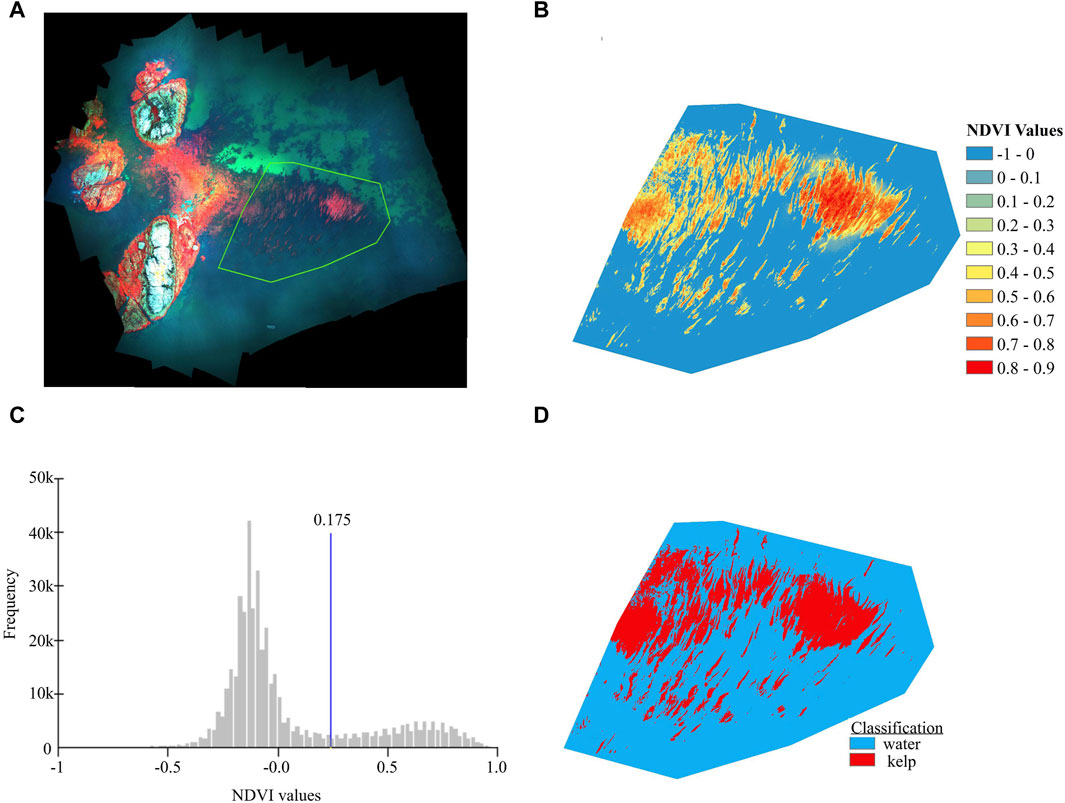
FIGURE 3. An example of the kelp classification workflow, starting with (A) the full orthomosaic shown in false-color infrared (where the near-infrared band is shown in red) and a green outline showing the clipped kelp bed region used in the analysis, (B) the colour coded NDVI raster resulting from the clipped area, (C) the frequency histogram of the NDVI raster showing the Jenks natural breaks threshold in the trough between the water (lower) and kelp (higher) peaks, and (D) the resulting binary classification of kelp and water.
2.4 Statistical analyses
2.4.1 Evaluation of NDRE and NDVI for kelp canopy classification in UAV imagery
Exploratory analysis of the UAV imagery showed that NDRE classification (NDREUAV) detected considerably larger kelp extent than NDVI classification (NDVIUAV) in surveys with less than ∼150 square meters of kelp extent (mostly in imagery collected at tides >2 m). This discrepancy was due to smaller beds becoming almost entirely submerged at high tides and, consequently, less detectable with NDVIUAV (Timmer et al., 2022). Since most kelp remote sensing imagery is either collected at lower tides, or filtered for days when tides are low, with beds much more extensive than 150 square meters (e.g., a single Landsat pixel at 30 m2 representing an area of 900 square meters), VIn classifications were only compared for imagery with more than 150 m2 of kelp extent. As such, 10 of the 65 total orthomosaics were removed from the VIn comparisons and the area of classified kelp canopy (m2) was determined for the remaining beds using both NDVIUAV classification (areaNDVI) and NDREUAV classification (areaNDRE).
First, to determine which VIn detects more kelp, a pairwise t-test was used to compare the mean difference between areaNDRE and areaNDVI at the bed-level (Cohen, 1988); Then, to investigate whether these differences in kelp detection are (i) species specific (i.e., between Macrocystis and Nereocystis canopies) or (ii) different during higher (above 2 m) versus lower (below 2 m) tidal heights, the ratio between areaNDVI/areaNDRE was determined for each bed and two separate analyses were conducted. (i) A two-sample t-test was used to compare species level detection differences (Cohen, 1988); and (ii) the Welch’s t-test for unequal variance was used to compare detection differences at high versus low tides (Cohen, 1988). The appropriate statistical tests for each comparison were determined by first checking for normal distribution using the ShapiroWilk test and for equality of variance using an F-test (Cohen, 1988).
2.4.2 The effects of tidal height and current speed on NDVI classified kelp canopy extent
For this analysis, areaNDVI was chosen rather than areaNDRE as the measure of kelp extent, given that NDVI is the most commonly used vegetation index for kelp remote sensing due to the prevalence of the NIR band and lack of RE band in many satellite sensors (e.g., Landsat, Spot). The evaluation of tidal height and current speeds on the areaNDVI was determined according to multivariate regression for each of the eight kelp beds surveyed. Akaike Information Criterion with modification for small sample size (AICc) was used to rank the importance of tidal height and current speed in determining kelp extent (Burnham and Anderson, 2004). The multivariate regression results were ranked for each bed instead of one global model because the canopy extents and minimum tidal heights of each bed were different. This analysis considered classified “canopy extent” (i.e., areaNDVI) as the dependent variable with either “tidal height” and/or “current speed” as the independent variable(s) (Faraway, 2002), with both additive and interactive effects of these factors considered, where possible. Unfavourable environmental conditions (large swell and excessive glint) during UAV imagery acquisition resulted in a lower number of degrees of freedom (i.e., useable orthomosaics) for two of the eight kelp beds (TA_1, df = 5; TA_2, df = 4). Therefore, the AICc ranking for TA_1 did not include interactive effects between tide and current, and the ranking for TA_2 did not include additive or interactive effects. In addition to ranking models with AICc, variance inflation factors were used to quantify the strength of the correlation between tidal height and current speed at each site (Cohen, 1988; Stine, 1995).
A second level of analysis was conducted to define the rate of change for areaNDVI due to tidal height increases, ignoring in situ current speeds. For this analysis, the relationship between tidal height (x) and areaNDVI (y) for each bed was defined using simple linear regression models. Since the total extent of each kelp bed varied between sites, the tide-extent relationships were standardized by dividing the slope of each linear equation (m) by the y-intercept (b), which provided the decrease in canopy extent per meter as a percentage of the estimated kelp extent at 0 m tidal height (Eq. 4).
This standardization relied on the assumption that all estimates of the y-intercept were reasonably accurate (see Table 3 in Results for r2 values) and that the extent at 0 m tidal height was a reasonable benchmark representing 100% of possible kelp canopy at the surface. Once the data was standardized, the tide-extent relationships for individual kelp beds were characterized using the average values (mean ± SD) and the overall ranges of slopes. These descriptive statistics were determined at the species level, as well as between high-current (>10 cm/s) and low-current (<10 cm/s) sites.
3 Results
3.1 Spatial and temporal water characteristics
Before spectral comparisons can be made for kelp at the structure or bed levels, it is important to verify that the spectral properties of the surrounding waters are not a confounding factor between sites and days of surveys in the analyses. Here, the optical constituents and optical properties of the water had generally low spatial (between site) and temporal (between days) variability (Table 2). TSM concentrations (3.3 ± 0.3 mg/L; with similar contributions of inorganic PIM: 58.8% ± 4.2% and organic POM:41.2% ± 4.22%) and Secchi depths (4.1 ± 1.1 m) showed that turbidity was relatively low during the survey days, in comparison with reported TSM in a large range of coastal waters in BC (Phillips and Costa, 2017).
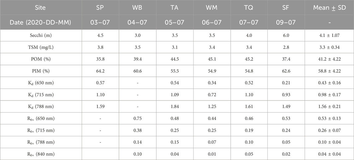
TABLE 2. Water optical properties and parameters for deep water at each site and averages over the survey period. TSM = total suspended matter; POM = percent organic matter; PIM = percent inorganic matter; Kd = diffuse attenuation coefficient; R0+ = above-water reflectance. Site codes are in Figure 1.
The low concentrations and variability of suspended particulate matter are also expressed in the low R0+ and Kd values. For deep-water (Figure 4A; Table 2), R0+ was most variable in the blue and green wavelengths, with the red, RE, and NIR wavelengths showing relatively low R0+ and minor differences between sites. The deep-water spectra showed a strong R0+ peak at 570 nm and a small fluorescence peak at ∼690 nm, yet none of the spectra had peaks in the RE or NIR that would have indicated high water turbidity due to a phytoplankton bloom or high concentrations of inorganic particulates (Kutser, 2009; Phillips and Costa, 2017). The Kd values indicated that light attenuation in the water column generally increased at longer wavelengths (Figure 4B; Table 2), with the NIR (788 nm) values roughly 1.5 times higher than in the RE (715 nm), and the RE was about twice as high as in the red wavelengths (650 nm). Together, this dataset indicates that turbidity was low during all surveys, and consequently, low variability in both R0+ and Kd was observed. Therefore, the spectral properties of the water are not expected to substantially add to the R0+ variability of the kelp in our analyses.
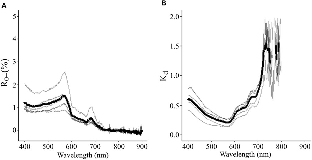
FIGURE 4. Summary of (A) the percentage of light reflectance (R0+) between 400 and 900 nm from deep-water spectra during surveys and (B) Diffuse attenuation coefficient (Kd) between 400 and 800 nm for the top meter of the water column during surveys. For each, the thick black line indicates the mean values over the survey period, and the grey lines show the variability of measurements between days.
3.2 In situ spectral characterization of morphologically different kelp structures
The in situ above-water spectra showed that the morphology and buoyancy of different kelp canopy structures play an important role in the resulting above-water spectra. The locations of spectral peaks were generally similar regardless of structure type (pneumatocyst, frond, or blade), but the magnitude of R0+ in the RE and NIR varied considerably for each structure type (Figure 5A). In the visible region of the spectrum (400–700 nm), all structure types had similar shapes and magnitude of spectral peaks at 575, 600, and 645 nm. These similarities were likely due to shared photosynthetic and accessory pigments, with both Nereocystis and Macrocystis species having a combination of chlorophyll-a, chlorophyll-c, and fucoxanthin pigments (Duncan, 1973; Wheeler, 1980). Additionally, each spectra showed a peak at the top of the RE (∼715 nm) and a second peak higher in the NIR (∼815 nm) for all kelp structures, yet the magnitude of these peaks varied for each structure type. When out of the water, the R0+ of different kelp species are highly similar (Supplementary Material S5) and often the R0+ of structures only vary by around 5% (Timmer et al., 2022), and since the structures here were aggregated at high densities within the sensor’s field of view, in situ differences in the shape and magnitude of R0+ signal are thought to be mainly due to their differing buoyancies and resulting levels of submergence below the water’s surface.
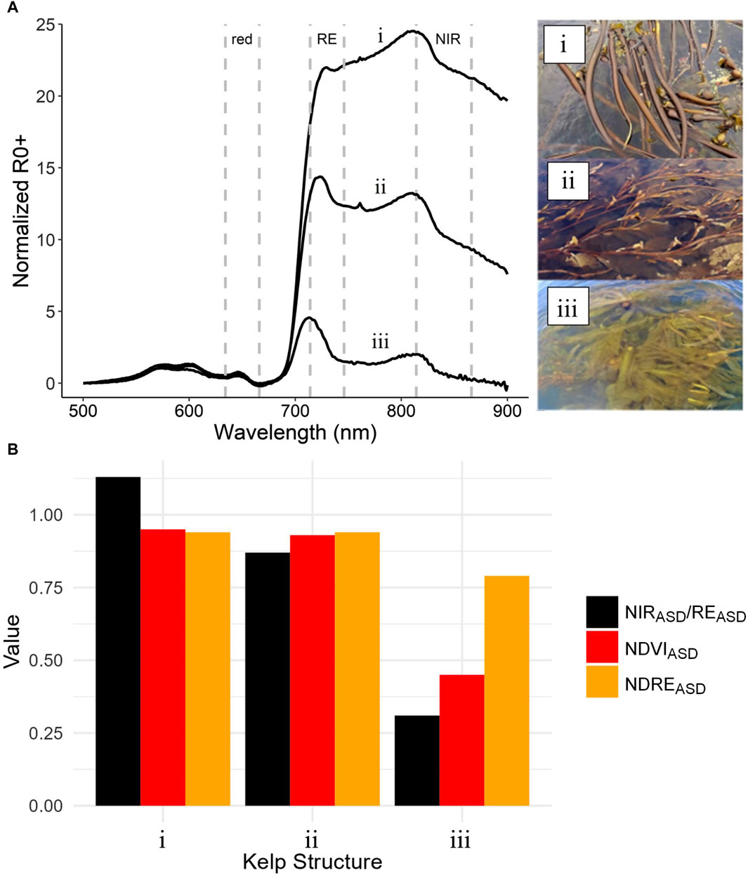
FIGURE 5. (A) In situ spectra (mean value) and spectral targets for dense examples of (i) Nereocystis pneumatocysts, (ii) Macrocystis fronds, and (iii) Nereocystis blades. Spectra have overlayed red, red-edge (RE), and near-infrared (NIR) bandwidths of the DJI Phantom 4 multispectral sensor, which were used to simulate multispectral band reflectance signals and calculate (B) NIR/RE ratios and vegetation indices for each structure type.
Nereocystis pneumatocysts were highly buoyant, and a relatively large portion of their biomass remained emergent above the water (Figure 5Ai), resulting in the highest overall reflectance and a more prominent NIR peak compared to the RE peak. Portions of the Macrocystis fronds were buoyant because of their multiple small pneumatocysts, but the majority of frond biomass (e.g., blades and stipes) remained submerged just below the surface of the water (Figure 5Aii), resulting in a lower overall reflectance than the Nereocystis pneumatocysts and a more prominent RE peak compared to the NIR peak. The Nereocystis blades were not buoyant and remained just below the water surface (Figure 5Aiii), resulting in the lowest overall spectral signal and a more prominent RE peak compared to the NIR peak.
The in situ R0+-based simulated multispectral bands of the DJI UAV showed similar values as the hyperspectral REASD and NIRASD R0+. However, the derived NDVIASD and NDREASD for both Nereocystis pneumatocysts and Macrocystis fronds were very near to the maximum possible VIn value of 1.0 (Figure 5B), despite the differences in the overall magnitude of R0+ at the REASD and NIRASD bands regions (Figures 5Ai, ii). Conversely, for the Nereocystis blades that were entirely submerged, the R0+ at the REASD and NIRASD bands were only slightly higher than the R0+ at the redASD band (Figure 5Aiii). As such, the VIn values for blades were substantially lower than those of the other structures, with NDREASD values being nearly twice that of the NDVIASD (Figure 5B).
3.3 Bed level comparison of UAV based NDRE and NDVI classifications
Across all UAV surveys, the data showed that areaNDRE was larger than areaNDVI (t = 7.17, df = 58, p-value <0.001) regardless of the species surveyed (t = −0.07, df = 51, p-value = 0.95) or tidal height during the survey (t = −0.54, df = 27.7, p-value = 0.59). The summed total of areaNDRE was 18% larger than the areaNDVI across all beds. Despite NDREUAV detecting larger kelp extent than NDVIUAV, there were no significant differences (t = 0.49, df = 14, p-value = 0.635) between the rate of decrease for canopy extent classified with NDREUAV (mean ± SD: −24.3% ± 5.3%/m) or with NDVIUAV (−25.7% ± 6.6%/m), indicating that similar relationships can be expected in our tide and current analysis using either a NDREUAV or NDVIUAV classification. A simple visual comparison of the NDREUAV and NDVIUAV classifications made it apparent that the reason for this difference was related to the additional NDREUAV-classified kelp area being consistently at the edges of the kelp bed.
For instance, Figure 6 shows three orthomosaics from the same region of the Womanley Macrocystis bed (see Figure 1 for location) collected at low (0.2 m), medium (1.7 m), and high (3.2 m) tidal height; each with a simple overlap of NDREUAV classified areaNDRE and NDVIUAV classified areaNDVI using a fixed threshold of 0. At each tidal height, the additional NDREUAV-classified kelp can be seen at the edges of the fronds, contributing to the overall larger areaNDRE. Quantitatively, the NDVIUAV and NDREUAV values of 2 m × 2 m regions crossing the kelp bed from west to east showed that, at each tidal height, both NDVIUAV and NDREUAV values were higher (mean ± SD) at the center of the kelp bed and lower towards the bed edges, suggesting a higher kelp density at the bed centre. In addition, regardless of the position across the kelp bed, the NDREUAV values are higher than NDVIUAV because much of the Macrocystis biomass is just below the water’s surface. Therefore, the higher RE signal from kelp at the bed edges allowed some pixels to be classified with NDREUAV but not NDVIUAV.
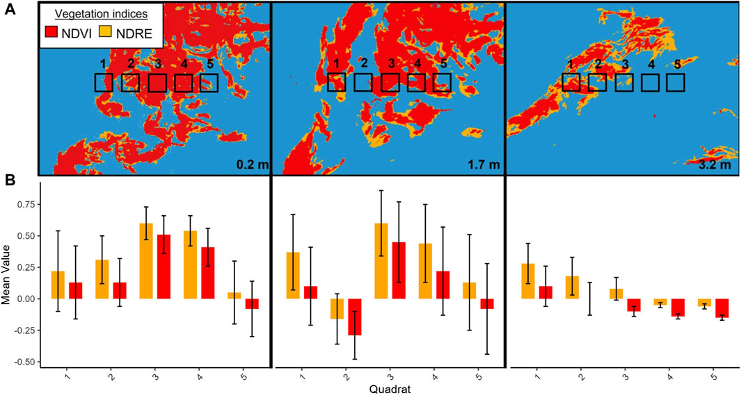
FIGURE 6. (A) NDRE (orange) and overlayed NDVI (red) classified Macrocystis from a subsection of the Womanley kelp bed at tidal heights of 0.2, 1.7, and 3.2 m. Five quadrat areas (each 2 m2 for scale between panels) overlay the classified kelp at the same georeferenced coordinates, although the kelp canopy appears to move due to local currents within the site (e.g., at 3.2 m tide). Panels show only a small portion of the total kelp bed and are not meant to reflect the full bed extent at each tidal height. (B) The NDVI and NDRE values (mean ± SD) for each quadrat area are listed below each panel as a barplot.
3.4 Kelp extent: tide and current relationships
The best fit model for seven of the eight kelp beds surveyed contained tidal height alone as predictor for areaNDVI kelp extent (Supplementary Material S6). For the eighth bed (TA_1), both current and tidal height were equal predictors of areaNDVI. However, for both TA_1 and TA_2, tidal height and current speed were highly correlated throughout the surveys (VIF >10), and therefore these two variables were highly collinear and, therefore, the model results cannot be interpreted with confidence. Since tidal height was the only variable strongly supported by all AICc comparisons, further analysis was conducted for all beds using this variable alone as predictor of areaNDVI.
Linear regression models between areaNDVI and tidal height showed strong negative linear relationships for all eight kelp beds surveyed (Table 3). For all beds, tidal height alone was strongly correlated with areaNDVI (R2 > 0.90), with an average decrease in detected kelp canopy extent of about −26% per meter of tidal height increase. The areaNDVI of beds that were subjected to high current speeds (>10 cm/s; TA1 and TA2) decreased at nearly twice the rate (−35.5% per meter) of the beds at the lower current (<10 cm/s) sites (−22.5% per meter). This suggests a strong interaction between tidal height and currents at these high current Nereocystis sites, that could not be verified statistically due to low degrees of freedom and high collinearity. At the third Nereocystis bed (SF_N, <10 cm/s), the areaNDVI decreased at a similar rate to the other Macrocystis beds and the mixed bed (Table 3). Overall, the rate of decrease for the detected canopy extent of the three Nereocystis beds was nearly three times greater than for the three Macrocystis beds (Table 4). However, rates of decrease for detected canopy extent were roughly similar and predictable between both species in low-current environments.
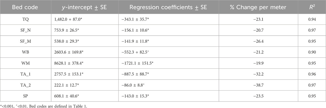
TABLE 3. Intercept (±SE) and regression coefficient (±SE) for linear regression models using only tidal height as a predictor variable, as well as the coefficient of variation (R2) for each model.
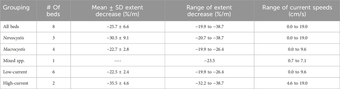
TABLE 4. Descriptive statistics of NDVI-derived kelp bed extent (areaNDVI) characteristics grouped by both species and current speed.
4 Discussion
Accurately measuring kelp canopy extent with remote sensing requires consideration of numerous variables at the planning, acquisition, and analysis stages of kelp mapping. Here, in situ hyperspectral data paired with field observations demonstrated that differing buoyancy between kelp structures resulted in variable R0+ at the RE and NIR wavelengths. Further, multispectral UAV imagery showed that NDRE classification detected 18% more kelp extent than NDVI classification, regardless of species or tide levels. This difference in detection was most apparent near the edges of the kelp beds, where kelp structures were often submerged. Ultimately, measured kelp extent showed a strong negative linear relationship with tidal height, decreasing at an average of 25.7% ± 6.6% per meter of increase in tidal height. However, further analysis showed that low-current beds decreased at an average of 22.5% per meter and high-current beds decreased at an average of 35.5% per meter, suggesting more investigation is needed into the interactive effects of high current speeds and tidal height on kelp submersion.
4.1 Spectral characterization of water and kelp canopy at the structure and bed scales
Different kelp canopy structures, and even kelp species, are generally grouped as a single class in remote sensing imagery, with variability in R0+ associated with changes in density (Schroeder et al., 2019a; Nijland et al., 2019; Bell et al., 2020a). However, our results show that for different kelp structures, the R0+ at the NIR and RE wavelengths also vary according to the amount of emergent kelp at the water’s surface (Figure 5), which is a result of the buoyancy of the kelp structures and their spatial distribution within a kelp bed, i.e., bed centre or edges (Figure 6). Generally, when kelp is emergent above the water surface, the NIR signal is slightly higher than the RE signal, regardless of structure type (Timmer et al., 2022). If submerged even slightly, the RE signal quickly becomes higher than the NIR signal because the R0+ at RE wavelengths are much less attenuated by water and its optical constituents than at the NIR wavelengths (Timmer et al., 2022). In this study, the spectral properties of the water were similar between all surveys, and therefore the differences in kelp R0+ were primarily attributed to variability within and between kelp beds rather than changes in water optical properties. However, it is important to note that different optical conditions of water may yield varying results for kelp detection and should still be considered when choosing spectral bands for kelp mapping.
Despite the differences in RE and NIR attenuation, the simulated multispectral UAV data showed that both NDREASD and NDVIASD values were positive regardless of the kelp structure, meaning that both VIn can still accurately classify dense kelp canopy structures if they are at or just below the water’s surface. Nonetheless, in the UAV imagery, NDREUAV detected ∼18% more kelp overall at the bed level, indicating that a portion of the kelp canopy was submerged deeper than the NDVIUAV could detect but still within the detection limits of the NDREUAV.
Spatially, both NIRUAV and REUAV reflectance signals were consistently lower at the bed periphery relative to the bed center. Yet the REUAV signal here was generally higher than NIRUAV (Figure 6), which suggested that the reduced NIRUAV signal was likely due to submersion rather than lower density of kelp. The higher REUAV signal from kelp at the bed edges allowed some pixels to be classified with NDREUAV but not NDVIUAV. Together, these examples demonstrate that both NDVI and NDRE may accurately classify dense kelp at the center of a bed where VIn values are consistently higher, while kelp at the bed edges may be more accurately classified using NDRE due to the improved detectability of submerged kelp. We were unable to measure why kelp was more submerged at the bed periphery, but we hypothesize that it may be due to slightly higher current speeds at the bed-edge submerging more canopy than at the center of the bed where currents are reduced (Monismith et al., 2022). This level of analysis is important for when deriving kelp bed biomass based on NDVI (K. Cavanaugh et al., 2011) because our results suggest that dense kelp at the periphery of a bed will have a lower NIR R0+ if submerged. Therefore, incorporating RE bands into classification schemes may be useful for detecting more biomass of submerged kelp structures such as Nereocystis blades, and for understanding variable R0+ between sparse and submerged kelp canopy. In these cases, the ability to detect deeper submerged kelp canopy will vary based on the R0+ magnitude for each kelp structure, the bio-optical properties of the water, and the depth at which the structure is submerged, making it important to understand and consider in situ environmental factors.
4.2 Tide and current analysis
The same increases in tidal height resulted in both a higher and more variable rate of decrease in classified kelp canopy extent for Nereocystis beds (−30.5% ± 9.1%/m) than for Macrocystis beds (−22.7% ± 2.8%/m) or the mixed bed (−23.5%/m). These differences are likely due to the wide range of current speeds during UAV flights at the Nereocystis sites (0.0–19.0 cm/s) versus the narrower range measured at Macrocystis sites (0.0–9.6 cm/s) and the mixed site (0.7–7.1 cm/s). When considering only low-current speed data (<10.0 cm/s), the canopy extents decreased at a similar rate (−22.5% ± 2.4%/m) for all sites, regardless of species. Under these low-current conditions, despite the distinct morphologies of Macrocystis and Nereocystis, the buoyant forces that result from the pneumatocysts and fronds hold the kelp canopy at or near the water’s surface. As the tidal height increases, the basal ends of the floating portion of the surface canopy (Macrocystis frond or Nereocystis pneumatocyst) are held in place by the holdfast and pulled below the water’s surface at similar rates (Figure 7). This process takes place simultaneously for each individual within the kelp bed, and as a result, tidal height alone explained more than 90% of the variability in the canopy extent over the tidal cycle at low-current sites.
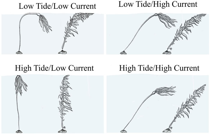
FIGURE 7. Observation based differences in the orientation of kelp structures during different combinations of tidal heights and current speeds. Bull kelp is on the left and giant kelp is on the right in each panel, and are not necessarily to scale.
Two of the Nereocystis beds surveyed were exposed to relatively higher current speeds, up to 19.0 cm/s. At these beds, the average rate of decrease (−35.5% ± 4.6%/m) was nearly twice that of the sites with lower current speeds (−22.5% ± 2.3%/m) (Table 4). Here, similar to beds in low-current conditions, the increasing tidal height submerges the basal portion of the kelp canopy. However, the high current adds horizontal drag to the kelp, pushing it diagonally into the water column and resulting in additional submersion of the canopy (Figure 7). Although it was not possible to test interactive effects between tide and current due to low degrees of freedom, it is reasonable to assume that faster current speeds at higher tides cause increased submersion compared to at lower tides due to the potential for increased drag.
In a similar study of Macrocystis remote sensing in California, tidal height also showed negative linear relationships (R2 = 0.72–0.98) with UAV-derived canopy extent (Cavanaugh et al., 2021b). Of the two California beds surveyed, the shallower bed showed a similar tide-extent relationship (−20.1%/m; max. depth 8 m) as the Macrocystis beds in our study (−22.7%/m; max. depth 5 m). However, the deeper Macrocystis bed decreased at nearly half the rate of the shallower bed (−12.7%/m; max. depth 16 m). Our findings suggest that the deeper bed’s lower rate of decrease in classified canopy extent may be due to local high current speeds (>20 cm/s) at lower tidal heights during surveys, which may have hidden the true maximum canopy extent. While current speed was not a significant predictor of kelp extent in their work, Cavanaugh et al. (2021b) note that the effect of current speed on classified kelp canopy area was large and suggested that with a larger sample size, current would have likely been a significant predictor of kelp extent.
In another study in the Strait of Juan de Fuca, Washington, which used oblique angle colour photography from land-based vantage points, extreme currents (>100.0 cm/s) resulted in Nereocystis canopy extent decreases between 50% to nearly 100% during a 1-m increase in tidal height (Britton-Simmons et al., 2008). Similar to our and Cavanaugh et al.‘s results, this study showed that currents below 10.0 cm/s did not affect classified canopy extent. Together, this body of knowledge suggests that although they may be difficult to track, local current speeds likely play a substantial role in kelp submersion at both high and low tidal heights and that their effects on measuring accurate kelp extent should be investigated further with UAV imagery.
4.3 Implications for satellite remote sensing of kelp extent
Our results describe the effects of tidal height and current speed on the extent of kelp canopy detected by a very high spatial resolution (∼5 cm) multispectral sensor at high temporal resolution (up to 9 times over a single tidal cycle). However, kelp forest mapping is often conducted using satellite imagery on a regional scale with either high (<10 m) or medium (10–30 m) spatial resolution imagery that are generally acquired at a lower temporal resolution (acquisition weeks or months apart). Therefore, our results should be considered in the context of the spatial and temporal differences typical of satellite imagery collection and analysis, such as multi-year time series using single low tide images acquired annually during peak kelp growth (Schroeder et al., 2019a; Gendall et al., 2023) or time series that aggregate results of all imagery acquired over a period of time (Bell et al., 2020a; K; Cavanaugh et al., 2011; Nijland et al., 2019). In either scenario, the relationships provided by this study are crucial to understand uncertainties associated with tidal height on the kelp canopy extent derived from satellite imagery.
For instance, Schroeder et al. (2019b) and Hamilton et al. (2020) used a maximum acceptable tidal height of ∼2.0 m as a threshold for Nereocystis detection with satellite imagery. Our results suggest that if these tidal conditions are selected in low-current areas, kelp canopy extent differences of 45% (i.e., 22.5% per meter) should be expected from imagery collected within that range. In such cases, it may be beneficial to select narrower tidal windows to allow the user to reduce uncertainties related to tidal heights, with lower tidal heights producing the most kelp canopy at the surface. However, a simple exercise using satellite-derived kelp extent by Nijland et al. (2019) shows that upscaling our results to satellite may not be straightforward. Nijland et al. (2019) acquired paired imagery of the same region at two different tidal heights with WorldView-2 (2 m spatial resolution; 1.5 and 3.6 m tidal height) and Landsat-8 (30 m spatial resolution; 0.6 and 2.7 m tidal height), each acquired roughly 1 month apart. This imagery was from an exposed group of islets (the McMullin group) just north of the kelp beds surveyed in this research, where large, dense, and contiguous Macrocystis beds occur at shallow depths (<5 m). After standardizing their results with ours (as in Section 2.4.2), kelp extent was estimated to decrease by 18%/m with WorldView-2, and 15%/m with Landsat-8 as tidal height increased. These values are lower than the average decrease for low-current sites in our higher spatial and temporal resolution study (−22.5%/m). One potential explanation for these differences is that the reduced rate of decrease is an artifact the thresholding methods used by Nijland et al. (2019) on the lower spatial resolution imagery. For example, in their methods, a pixel of Landsat imagery must contain only 20% kelp canopy fraction to be positively classified as a kelp (Nijland et al., 2019; Hamilton et al., 2020). As such, our data suggest that a satellite imagery pixel containing 100% kelp canopy at 0.0 m tide could decrease by 22.5%/m, and at 3.5 m tidal height could still be positively classified with the binary threshold in Nijland et al.’s (2019) methods. Therefore, as the spatial resolution of imagery decreases, using a binary threshold to classify large contiguous kelp beds may disproportionately overestimate canopy extent at higher tidal stages.
Regardless of the classification and mapping methods used in kelp remote sensing, it is crucial to collect accurate ground truth data to reduce potential errors in high to medium-resolution (<30 m) satellite imagery associated with different kelp structures and varying tidal heights. For example, a remote sensing pixel that contains 100% density of Nereocystis pneumatocysts generally has a higher reflectance signal than a pixel that contains the same percentage of Macrocystis fronds or Nereocystis blades. Therefore, if a Nereocystis pneumatocyst is used as an end-member for determining the fraction of fronds or blades within a pixel, the true kelp fraction for that pixel will be underestimated. Additionally, our results suggest that if multiple end-member spectral mixture analysis (MESMA) is used to estimate kelp biomass of Macrocystis within satellite resolution imagery (Cavanaugh et al., 2011), the availability of a RE band may allow for increasingly accurate biomass estimation due to the ability to detect submerged portions of the canopy more effectively. As such, the addition of RE bands or hyperspectral sensors on future remote sensing platforms will be of benefit to the remote sensing community for monitoring shallow submerged vegetation. There are many different considerations when choosing a remote sensing platform to monitor kelp, the breadth of which go beyond the scope of this research, but an openly available resource to narrow down best practices and options for effectively monitoring kelp is available to help make those decisions (https://catalogue.hakai.org/dataset/ca-cioos_c074bff6-408b-443a-bdaf-4713f0eadb95).
Conversely, in regions with shallow vegetation, classifying nearshore kelp in satellite imagery acquired during low tide requires the incorporation of known sources of uncertainties. For example, nearshore Macrocystis and Nereocystis kelp forests in BC often contain various species of understory vegetation, such as Pterygophora california, which forms a secondary benthic canopy up to 2 m off the sea floor (Shaffer, 2000; Druehl and Clarkston, 2016). Nearby our study sites, subtidal Pterygophora beds were mixed with shallow Macrocystis beds at two locations. In both cases, the Pterygophora canopy was detectable in UAV imagery with both NDRE and NDVI classification at 0.5 m tidal height, yet at 1.0 m tidal height, the Pterygophora canopy was only detectable with the NDRE. Therefore, to avoid overestimation of overstory kelp canopy extent due to misclassification of understory canopy, caution should be exercised when monitoring nearshore kelp beds at the lowest tides, especially with RE indices. NIR-based indices like NDVI may help reduce these potential errors by only detecting the kelp canopy nearest to the surface. Further, deeper than 1 m below the surface, even the NDRE will be unlikely to detect any understory kelp canopy (Timmer et al., 2022), making it unlikely that this region of the spectral range would be useful for mapping anything but the shallowest kelp canopies at the lowest tides. If specifically targeting only understory kelp canopy, the visible range of the spectrum is still the most useful.
5 Conclusion
Submergence of kelp canopy is associated with buoyancy differences between canopy structures, tidal height, and current speed, leading to changes in the detected R0+ and, therefore, derived kelp canopy extent. In this study, we described spectral characteristics that arise from morphological and bed-level differences between Macrocystis and Nereocystis, and we quantified the effects of local tides and currents on the apparent extent of Macrocystis and Nereocystis canopy when using remote sensing imagery. In situ submerged kelp structures showed lower overall R0+ than emergent structures but a higher relative R0+ in the RE than the NIR. The in situ hyperspectral data was supported by complimentary multispectral UAV imagery, which showed that kelp was more likely to be submerged at the periphery of the bed, possibly due to higher currents at the bed edges versus the bed center. Further, the vegetation index that relied on the R0+ of the RE wavelength (NDRE) detected 18% more submerged canopy than the NDVI, meaning that inclusion of RE bands or hyperspectral sensors on future remote sensing platforms could be advantageous for detecting shallow submerged vegetation. However, using red-edge indices may also overestimate kelp canopy extent due to the misclassification of shallow submerged benthic vegetation. At the bed level, our results are important to interpret trends across a range of tidal heights and currents by providing a range of possible errors associated with site-specific metrics of bed extent. Tidal height had a strong negative linear relationship with the canopy extent of both Macrocystis and Nereocystis at all sites, and in low-current areas (<10.0 cm/s), canopy extent decreased by an average (mean ± SD) of 22.5% ± 2.4%/m, regardless of species. Unlike Macrocystis, Nereocystis was found in both low and high current areas (>10.0 cm/s), and as such, Nereocystis canopy extent decreased at a higher and more variable rate (30.5% ± 9.1%/m) when compared to Macrocystis (22.7% ± 2.8%/m). Overall, we recommend minimizing the range of tidal conditions over which temporal analyses are conducted and incorporating an explicit understanding of the role of currents when comparing the detected extent of kelp beds either between sites or at sites with a large range of current speeds. This research contributes to improve the methodological framework used to map canopy kelp and understand the ongoing changes in kelp forest ecosystems globally. Remote sensing is a key tool for monitoring these changes, and, as such, it is critical to understand the implications of collecting remote sensing imagery of kelp forests at various tidal heights and current speeds.
Data availability statement
The datasets presented in this study can be found in online repositories. The names of the repository/repositories and accession number(s) can be found below: https://catalogue.hakai.org/erddap/index.html.
Author contributions
BT: Conceptualization, Data curation, Formal Analysis, Funding acquisition, Investigation, Methodology, Project administration, Writing–original draft. LR: Conceptualization, Investigation, Methodology, Project administration, Writing–review and editing. MH-L: Formal Analysis, Funding acquisition, Methodology, Resources, Supervision, Writing–review and editing. FJ: Resources, Supervision, Writing–review and editing. LG: Investigation, Visualization, Writing–review and editing. MC: Conceptualization, Formal Analysis, Funding acquisition, Methodology, Project administration, Supervision, Writing–review and editing.
Funding
The author(s) declare that financial support was received for the research, authorship, and/or publication of this article. During this research BT was supported through a MITACS Accelerate internship with the Hakai Institute, as well as an NSERC CGS-M award and MC’s NSERC-DG.
Acknowledgments
We thank the Hakai Institute, Mitacs Canada, and The Natural Sciences and Engineering Research Council of Canada for providing funding for this research. We also thank Kyle Cavanaugh for his insightful comments and suggestions during the preparation of this manuscript, and Jessy Barrette for his help working with the acoustic doppler current profiler, and providing code to work with the resulting tide and current data.
Conflict of interest
The authors declare that the research was conducted in the absence of any commercial or financial relationships that could be construed as a potential conflict of interest.
Publisher’s note
All claims expressed in this article are solely those of the authors and do not necessarily represent those of their affiliated organizations, or those of the publisher, the editors and the reviewers. Any product that may be evaluated in this article, or claim that may be made by its manufacturer, is not guaranteed or endorsed by the publisher.
Supplementary material
The Supplementary Material for this article can be found online at: https://www.frontiersin.org/articles/10.3389/fenvs.2024.1338483/full#supplementary-material
References
Arafeh-Dalmau, N., Montaño-Moctezuma, G., Martínez, J. A., Beas-Luna, R., Schoeman, D. S., and Torres-Moye, G. (2019). Extreme marine heatwaves alter kelp forest community near its equatorward distribution limit. Front. Mar. Sci. 6 (499), 1–18. doi:10.3389/fmars.2019.00499
Augenstein, E. W., Stow, D., and Hope, A. (1991). Evaluation of SPOT HRV-XS data for kelp resource inventories. Photogrammetric Eng. Remote Sens. 57 (5), 501–509.
Barsi, J. A., Lee, K., Kvaran, G., Markham, B. L., and Pedelty, J. A. (2014). The spectral response of the landsat-8 operational land imager. Remote Sens. 6 (10), 10232–10251. Article 10. doi:10.3390/rs61010232
Bell, T. W., Allen, J. G., Cavanaugh, K. C., and Siegel, D. A. (2020a). Three decades of variability in California’s giant kelp forests from the Landsat satellites. Remote Sens. Environ. 238, 110811. doi:10.1016/j.rse.2018.06.039
Bell, T. W., Nidzieko, N. J., Siegel, D. A., Miller, R. J., Cavanaugh, K. C., Nelson, N. B., et al. (2020b). The utility of satellites and autonomous remote sensing platforms for monitoring offshore aquaculture farms: a case study for canopy forming kelps. Front. Mar. Sci. 7, 1083. doi:10.3389/fmars.2020.520223
Britton-Simmons, K., Eckman, J. E., and Duggins, D. O. (2008). Effect of tidal currents and tidal stage on estimates of bed size in the kelp Nereocystis luetkeana. Mar. Ecol. Prog. Ser. 355, 95–105. doi:10.3354/meps07209
Burnett, N. P., and Koehl, M. A. R. (2017). Pneumatocysts provide buoyancy with minimal effect on drag for kelp in wave-driven flow. J. Exp. Mar. Biol. Ecol. 497, 1–10. doi:10.1016/j.jembe.2017.09.003
Burnham, K. P., and Anderson, D. R. (2004). Multimodel inference: understanding AIC and BIC in model selection. Sociol. Methods and Res. 33 (2), 261–304. doi:10.1177/0049124104268644
Burt, J. M., Tinker, M. T., Okamoto, D. K., Demes, K. W., Holmes, K., and Salomon, A. K. (2018). Sudden collapse of a mesopredator reveals its complementary role in mediating rocky reef regime shifts. Proc. R. Soc. B Biol. Sci. 285 (1883), 20180553. doi:10.1098/rspb.2018.0553
Butler, C., Lucieer, V., Wotherspoon, S., and Johnson, C. (2020). Multi-decadal decline in cover of giant kelp Macrocystis pyrifera at the southern limit of its Australian range. Mar. Ecol. Prog. Ser. 653, 1–18. doi:10.3354/meps13510
Casella, E., Collin, A., Harris, D., Ferse, S., Bejarano, S., Parravicini, V., et al. (2017). Mapping coral reefs using consumer-grade drones and structure from motion photogrammetry techniques. Coral Reefs 36 (1), 269–275. doi:10.1007/s00338-016-1522-0
Cavanaugh, K., Siegel, D., Reed, D., and Dennison, P. (2011). Environmental controls of giant-kelp biomass in the santa barbara channel, California. Mar. Ecol. Prog. Ser. 429, 1–17. doi:10.3354/meps09141
Cavanaugh, K. C., Bell, T., Costa, M., Eddy, N. E., Gendall, L., Gleason, M. G., et al. (2021a). A review of the opportunities and challenges for using remote sensing for management of surface-canopy forming kelps. Front. Mar. Sci. 8, 1536. doi:10.3389/fmars.2021.753531
Cavanaugh, K. C., Cavanaugh, K. C., Bell, T. W., and Hockridge, E. G. (2021b). An automated method for mapping giant kelp canopy dynamics from UAV. Front. Environ. Sci. 8, 587354. doi:10.3389/fenvs.2020.587354
Cohen, J. (1988). Statistical power analysis for the behavioral Sciences. 2nd ed. Hillsdale, NJ: Routledge. doi:10.4324/9780203771587
Dekker, A. G., Brando, V. E., and Anstee, J. M. (2005). Retrospective seagrass change detection in a shallow coastal tidal Australian lake. Remote Sens. Environ. 97 (4), 415–433. doi:10.1016/j.rse.2005.02.017
Druehl, L. D., and Clarkston, B. (2016). Pacific seaweeds: updated and expanded edition. Madeira Park, BC: Harbour Publishing.
Druehl, L. D., and Wheeler, W. N. (1986). Population biology of Macrocystis integrifolia from British Columbia, Canada. Mar. Biol. 90 (2), 173–179. doi:10.1007/BF00569124
Duncan, M. J. (1973). In situ studies of growth and pigmentation of the phaeophycean Nereocystis luetkeana. Helgoländer Wiss. Meeresunters. 24 (1–4), 510–525. doi:10.1007/BF01609538
Faraway, J. J. (2002). Practical regression and anova using R (vol. 168). Bath, UK: University of Bath.
Gallegos, C. L., Werdell, P. J., and McClain, C. R. (2011). Long-term changes in light scattering in Chesapeake Bay inferred from Secchi depth, light attenuation, and remote sensing measurements. J. Geophys. Res. Oceans 116 (C7). doi:10.1029/2011JC007160
Gendall, L., Schroeder, S. B., Wills, P., Hessing-Lewis, M., and Costa, M. (2023). A multi-satellite mapping framework for floating kelp forests. Remote Sens. 15 (5), 1276. Article 5. doi:10.3390/rs15051276
Giannini, F., Hunt, B. P. V., Jacoby, D., and Costa, M. (2021). Performance of OLCI sentinel-3A satellite in the Northeast Pacific coastal waters. Remote Sens. Environ. 256, 112317. doi:10.1016/j.rse.2021.112317
Hamilton, S. L., Bell, T. W., Watson, J. R., Grorud-Colvert, K. A., and Menge, B. A. (2020). Remote sensing: generation of long-term kelp bed data sets for evaluation of impacts of climatic variation. Ecology 101, e03031. doi:10.1002/ecy.3031
Jackson, J. M., Thompson, R. E., Brown, L. N., Willis, P. G., and Borstad, G. A. (2015). Satellite chlorophyll off the British Columbia coast, 1997–2010. J. Geophys. Res. Oceans 120, 4709–4728. doi:10.1002/2014jc010496
Jensen, J. R. (1980). Remote sensing techniques for kelp surveys. Photogrammetric Eng. Remote Sens. 46 (6), 743–755.
Karpouzli, E., and Malthus, T. (2003). The empirical line method for the atmospheric correction of IKONOS imagery. Int. J. Remote Sens. 24 (5), 1143–1150. doi:10.1080/0143116021000026779
Koehl, M. A. R., Silk, W. K., Liang, H., and Mahadevan, L. (2008). How kelp produce blade shapes suited to different flow regimes: a new wrinkle. Integr. Comp. Biol. 48 (6), 834–851. doi:10.1093/icb/icn069
Krumhansl, K. A., Okamoto, D. K., Rassweiler, A., Novak, M., Bolton, J. J., Cavanaugh, K. C., et al. (2016). Global patterns of kelp forest change over the past half-century. Proc. Natl. Acad. Sci. 113 (48), 13785–13790. doi:10.1073/pnas.1606102113
Krumhansl, K. A., and Scheibling, R. (2012). Production and fate of kelp detritus. Mar. Ecol. Prog. Ser. 467, 281–302. doi:10.3354/meps09940
Kutser, T. (2009). Passive optical remote sensing of cyanobacteria and other intense phytoplankton blooms in coastal and inland waters. Int. J. Remote Sens. 30 (17), 4401–4425. doi:10.1080/01431160802562305
Kutser, T., Vahtmäe, E., Paavel, B., and Kauer, T. (2013). Removing glint effects from field radiometry data measured in optically complex coastal and inland waters. Remote Sens. Environ. 133, 85–89. doi:10.1016/j.rse.2013.02.011
Loos, E. A., and Costa, M. (2010). Inherent optical properties and optical mass classification of the waters of the Strait of Georgia, British Columbia, Canada. Prog. Oceanogr. 87 (1–4), 144–156. doi:10.1016/j.pocean.2010.09.004
Mann, K. H. (1973). Seaweeds: their productivity and strategy for growth. Science 182 (4116), 975–981. Retrieved from:. doi:10.1126/science.182.4116.975
McHenry, J., Okamoto, D. K., Filbee-Dexter, K., Krumhansl, K., MacGregor, K. A., Hessing-Lewis, M., et al. (2024). A blueprint for national assessments of the blue carbon capacity of kelp forests applied to Canada's coastline.
Monismith, S. G., Alnajjar, M. W., Woodson, C. B., Boch, C. A., Hernandez, A., Vazquez-Vera, L., et al. (2022). Influence of kelp forest biomass on nearshore currents. J. Geophys. Res. Oceans 127 (7), e2021JC018333. doi:10.1029/2021JC018333
Mora-Soto, A., Palacios, M., Macaya, E. C., Gómez, I., Huovinen, P., Pérez-Matus, A., et al. (2020). A high-resolution global map of giant kelp (Macrocystis pyrifera) forests and intertidal green algae (ulvophyceae) with sentinel-2 imagery. Remote Sens. 12 (694), 694. Article 4. doi:10.3390/rs12040694
Murray, C., Markager, S., Stedmon, C. A., Juul-Pedersen, T., Sejr, M. K., and Bruhn, A. (2015). The influence of glacial melt water on bio-optical properties in two contrasting Greenlandic fjords. Estuar. Coast. Shelf Sci. 163, 72–83. doi:10.1016/j.ecss.2015.05.041
Mutanga, O., and Skidmore, A. K. (2004). Hyperspectral band depth analysis for a better estimation of grass biomass (Cenchrus ciliaris) measured under controlled laboratory conditions. Int. J. Appl. Earth Observation Geoinformation 5 (2), 87–96. doi:10.1016/j.jag.2004.01.001
Nahirnick, N. K., Hunter, P., Costa, M., Schroeder, S., and Sharma, T. (2019). Benefits and challenges of UAS imagery for eelgrass (zostera marina) mapping in small estuaries of the Canadian west coast. J. Coast. Res. 35 (3), 673. doi:10.2112/JCOASTRES-D-18-00079.1
Nijland, W., Reshitnyk, L., and Rubidge, E. (2019). Satellite remote sensing of canopy-forming kelp on a complex coastline: a novel procedure using the Landsat image archive. Remote Sens. Environ. 220, 41–50. doi:10.1016/j.rse.2018.10.032
Olson, A. M., Hessing-Lewis, M., Haggarty, D., and Juanes, F. (2019). Nearshore seascape connectivity enhances seagrass meadow nursery function. Ecol. Appl. 29 (5), e01897. doi:10.1002/eap.1897
O’Neill, J. D., and Costa, M. (2013). Mapping eelgrass (Zostera marina) in the Gulf Islands National Park Reserve of Canada using high spatial resolution satellite and airborne imagery. Remote Sens. Environ. 133, 152–167. doi:10.1016/j.rse.2013.02.010
O’Neill, J. D., Costa, M., and Sharma, T. (2011). Remote sensing of shallow coastal benthic substrates: in situ spectra and mapping of eelgrass (Zostera marina) in the gulf islands national park reserve of Canada. Remote Sens. 3 (5), 975–1005. Article 5. doi:10.3390/rs3050975
Pfister, C. A., Berry, H. D., and Mumford, T. (2017). The dynamics of kelp forests in the Northeast Pacific ocean and the relationship with environmental drivers. J. Ecol. 106 (4), 1520–1533. doi:10.1111/1365-2745.12908
Phillips, S. R., and Costa, M. (2017). Spatial-temporal bio-optical classification of dynamic semi-estuarine waters in western North America. Estuar. Coast. Shelf Sci. 199, 35–48. doi:10.1016/j.ecss.2017.09.029
RD Instruments (2005). RDI ADCP WorkHorse technical manual- april 2005.pdf. https://epic.awi.de/40219/1/ADCP_Sentinel_User_Guide.pdf.
Schroeder, S. B., Boyer, L., Juanes, F., and Costa, M. (2019a). Spatial and temporal persistence of nearshore kelp beds on the west coast of British Columbia, Canada using satellite remote sensing. Remote Sens. Ecol. Conservation 6, 327–343. doi:10.1002/rse2.142
Schalles, J. F., Gitelson, A. A., Yacobi, Y. Z., and Kroenke, A. E. (1998). Estimation of chlorophyll a from time series measurements of high spectral resolution reflectance in an eutrophic lake. J. Phycol. 34 (2), 383–390. doi:10.1046/j.1529-8817.1998.340383.x
Schroeder, S. B., Dupont, C., Boyer, L., Juanes, F., and Costa, M. (2019b). Passive remote sensing technology for mapping bull kelp (Nereocystis luetkeana): a review of techniques and regional case study. Glob. Ecol. Conservation 19, e00683. doi:10.1016/j.gecco.2019.e00683
Shaffer, J. A. (2000). Seasonal variation in understory kelp bed habitats of the Strait of juan de Fuca. J. Coast. Res. 16 (3), 768–775.
Springer, Y., Hays, C., Carr, M. H., and Mackey, M. (2007). ECOLOGY and management of the bull kelp, nereocystis luetkeana: a synthesis with recommendations for future research. Washington, DC: Lenfest Ocean Program, 1–53.
Starko, S., Neufeld, C. J., Gendall, L., Timmer, B., Campbell, L., Yakimishyn, J., et al. (2022). Microclimate predicts kelp forest extinction in the face of direct and indirect marine heatwave effects. Ecol. Appl. 32 (7), e2673. doi:10.1002/eap.2673
Stine, R. A. (1995). Graphical interpretation of variance inflation factors. Am. Statistician 49 (1), 53–56. doi:10.1080/00031305.1995.10476113
Sutherland, I. R. (2008). Kelp inventory, 2007: Areas of the British Columbia central Coast from Hakai Passage to the bardswell group (KELP INVENTORY). Canada: Ministry of Environment, 63. http://www.llbc.leg.bc.ca/public/PubDocs/bcdocs/454009/Kelp2007-HakaiPass.pdf.
Thomson, R. E. (1981). Oceanography of the British Columbia coast. Sidney, BC: Dept. of Fisheries and Oceans.
Timmer, B., Reshitnyk, L. Y., Hessing-Lewis, M., Juanes, F., and Costa, M. (2022). Comparing the use of red-edge and near-infrared wavelength ranges for detecting submerged kelp canopy. Remote Sens. 14 (9), 2241. Article 9. doi:10.3390/rs14092241
Tucker, C. J. (1978). A comparison of satellite sensor bands for vegetation monitoring. Photogrammetric Eng. Remote Sens. 44 (11), 1369–1380.
Wernberg, T., Krumhansl, K., Filbee-Dexter, K., and Pedersen, M. F. (2019). “Status and trends for the world’s kelp forests,” in World seas: an environmental evaluation (Elsevier), 57–78. doi:10.1016/B978-0-12-805052-1.00003-6
Keywords: remote sensing, kelp, tides, currents, multispectral, hyperspectral
Citation: Timmer B, Reshitnyk LY, Hessing-Lewis M, Juanes F, Gendall L and Costa M (2024) Capturing accurate kelp canopy extent: integrating tides, currents, and species-level morphology in kelp remote sensing. Front. Environ. Sci. 12:1338483. doi: 10.3389/fenvs.2024.1338483
Received: 14 November 2023; Accepted: 28 February 2024;
Published: 07 March 2024.
Edited by:
Dimitris Poursanidis, Foundation for Research and Technology Hellas (FORTH), GreeceReviewed by:
Meredith L. McPherson, University of Massachusetts Boston, United StatesCaitlin Blain, The University of Auckland, New Zealand
Copyright © 2024 Timmer, Reshitnyk, Hessing-Lewis, Juanes, Gendall and Costa. This is an open-access article distributed under the terms of the Creative Commons Attribution License (CC BY). The use, distribution or reproduction in other forums is permitted, provided the original author(s) and the copyright owner(s) are credited and that the original publication in this journal is cited, in accordance with accepted academic practice. No use, distribution or reproduction is permitted which does not comply with these terms.
*Correspondence: Brian Timmer, YnJpYW50aW1tZXJAdXZpYy5jYQ==