 Patrick Osei Darko1
 Etienne Laliberté2
 Margaret Kalacska1*
 J. Pablo Arroyo-Mora3
 Andrew Gonzalez4
 Juan Zuloaga4
- 1Applied Remote Sensing Laboratory, Department of Geography, McGill University, Montréal, QC, Canada
- 2Institut de Recherche en Biologie Végétale, Département de Sciences Biologiques, Université de Montréal, Montréal, QC, Canada
- 3Flight Research Laboratory, National Research Council of Canada, Ottawa, ON, Canada
- 4Department of Biology, McGill University, Montreal, QC, Canada
In collaboration with the International Union for the Conservation of Nature (IUCN) Taskforce on Biodiversity and Protected Areas, countries worldwide are working to develop a new systematic approach to inform the Key Biodiversity Areas (KBAs) initiative. The goal is to map KBAs from the national to global scales with a baseline international standard in support of biodiversity conservation efforts. According to the IUCN standard, one of the five criteria used to identify potential KBAs, is the Ecological Integrity (EI) of the ecosystem. Sites identified with respect to EI must have an intact ecological community and be characterized by minimal anthropogenic disturbance. In this study, a new EI metric, phenospectral similarity (PSpecM), has been developed and implemented in Google Earth Engine to identify potential forest stands of high EI from a large set of candidate stands. The implementation of PSpecM requires a network of known reference sites of high EI and target ecological units of the same land cover type for comparison to help identify potential sites of high EI. Here, we tested PSpecM on a ∼12,000 km2 study area in the Laurentian region, Quebec, Canada, using Sentinel-2 and PlanetScope (Dove) satellite imagery. Considering the phenological effect on reflectance, we found a 2,700 km2 spatial extent, equivalent to approximately 22% of the study area, commonly delineated as potential areas of high EI by both PlanetScope (Dove) and Sentinel-2. Without consideration of phenology, the total area delineated as potential areas of high EI increased to 5,505 km2, equivalent to around 45% of the study area. Our results show that PSpecM can be computed for rapid assessments of forest stands to identify potential areas of high EI on a large geographic scale and serve as an additional conservation tool that can be applied to the ongoing global and national identification of KBAs.
1 Introduction
Globally, we are facing a biodiversity decline at unprecedented rates due to direct and indirect impacts by humanity that is resulting in major economic and health impacts (e.g., food security and medicinal species) (Malcolm et al., 2006; Cardinale et al., 2012, Isbell et al., 2017). Human modification of forested lands and other ecosystems and the associated climate change impacts have been identified as key drivers of biodiversity loss worldwide (Schimel et al., 2013). There is an urgent need for a more sustainable approach for biodiversity management and conservation across the globe (Riera et al., 2020). For instance, Kullberg et al. (2019) expressed the need for a more efficient management approach of key habitats that support the maintenance and sustainability of biodiversity and wildlife populations. Such an approach should include the identification and conservation of a network of Key Biodiversity Areas (KBAs) to help minimize biodiversity loss and assist in conservation resources allocation (Eken et al., 2004; Schimel et al., 2013).
Despite the significant increase in protected sites in recent decades, biodiversity continues to decline (UNEP-WCMC and IUCN, 2021). The new Global Biodiversity Framework of the United Nations Convention on Biological Diversity adopted at COP15 has identified a target of protecting 30% terrestrial, inland water, and coastal and marine areas by 2030. Therefore, it has become increasingly important for policymakers to expand and adopt new measures to mitigate the declining biodiversity trends (Smith et al., 2019). To achieve this objective, the International Union for the Conservation of Nature (IUCN) Taskforce on Biodiversity and Protected Areas in collaboration with countries worldwide is developing a new and systematic approach for identifying KBAs (IUCN, 2016). The overarching goal is to map out KBAs at the national to global scales to support biodiversity conservation efforts with a baseline IUCN standard.
According to the IUCN standard, KBAs are “sites of importance for the global persistence of biodiversity” (IUCN, 2016). For a site to qualify as a KBA, it must meet one or more of the standardized IUCN criteria grouped under five categories (i.e., geographically restricted biodiversity, threatened biodiversity, ecological integrity, biological processes, and irreplaceability) (IUCN, 2016; Robertson et al., 2018). For instance, a forest stand identified with respect to ecological integrity (EI) must be characterized as a wholly intact ecological community (IUCN, 2016). Additionally, a candidate forest that is of high EI (i.e., intact ecological community) must demonstrate little to no natural or anthropogenic disturbance of the forest structure, species composition, and function (IUCN, 2016). This is because forest disturbances have direct impacts on the vegetation cover and can influence the important ecosystem services they provide (DeFries et al., 2007; Huang, 2018). The preservation of biodiversity sustains ecosystem services such as carbon sequestration and climate regulation to help combat climate change and the associated global warming (Birdsey et al., 2013). As deforestation escalates, carbon is released into the atmosphere to cause both an increase in the atmospheric concentration of carbon dioxide (greenhouse gas emissions) and a reduction in the sequestration potential of forests (DeFries et al., 2007; Lawrence et al., 2022; Nunes, 2023). These ecosystem services among others are some of the benefits associated with forests with high EI, thus necessitating their identification and protection. Although, globally, over 16,000 KBAs have been delineated (KBA, 2021), KBA identification is still an ongoing process, with many identified KBAs currently unprotected (Butchart et al., 2012; Beresford et al., 2020). This also calls for periodic monitoring of the KBA status to help detect and mitigate biodiversity disturbance.
Several methods have been used for the identification of KBAs to prioritize their conservation (Fraser et al., 2009; Reza and Abdullah, 2011; Jenkins et al., 2013; Kullberg et al., 2019; Li et al., 2020). These methods range from the use of the ranking of an area’s species richness at coarser spatial scales (e.g., 10 km × 10 km) (Jenkins et al., 2013) to local-scale biodiversity hotspot analysis (Meerman, 2007). Other studies have relied on existing tools such as the Management Effectiveness Tracking Tool (METT) (Stolton and Dudley, 2016) and Zonation conservation planning software (University of Helsinki, Finland) (Moilanen et al., 2014) for KBA assessments. Over the past decades, advancement in remote sensing technologies and the improved accessibility of remotely sensed data presents an opportunity to map KBAs to detect their periodic changes at different scales (Iverson et al., 1989; Toth and Jóźków, 2016). With these advancements (e.g., high spatial, spectral, and/or temporal resolutions), there is an opportunity to monitor the KBAs in near real time instead of the traditional one-time assessments to allow for cross-site comparisons over time (Beresford et al., 2020). Additionally, remote sensing offers a standard approach, which has been shown to be efficient for monitoring ecosystem changes for indications of landscape scale anthropogenic modifications (Rocchini, 2010; Nagendra et al., 2013; de Araujo Barbosa et al., 2015; Lamboj et al., 2019). The challenge, then, is to define a remotely sensed index that can capture important facets of the property of interest to be monitored, which in this case is EI.
The spectral reflectance of forest canopies from optical remotely sensed data can provide information about the vegetation’s compositional, functional, and structural variations to help characterize the vegetation structure and function (e.g., climate change effects and EI) across multiple spatiotemporal scales (Skidmore et al., 2021; Schweiger and Laliberté, 2022). For instance, Arroyo-Mora et al. (2018) employed Sentinel-2 (S2) multispectral satellite imagery to assess the short-term phenospectral (i.e., spectral variation as a function of phenological changes) dynamics of vegetation from a peatland ecosystem and found that these datasets can be useful for landscape scale detection of short-term phenological changes. In Canada, multitemporal Earth observation data have been used to monitor and assess the status and EI of the national parks at a landscape scale (Fraser et al., 2009). On the global scale, some efforts have focused on landscape scale quantification of forest EI (Grantham et al., 2020). By integrating multiple datasets such as the forest extent, observed and inferred human pressures, and alteration in forest connectivity, Grantham et al. (2020) quantified the Forest Landscape Integrity (FLI) index to describe the extent of forest alteration on a global scale. Beyer et al. (2020) also proposed a metric sensitive to habitat loss and fragmentation that can help delineate areas of high EI (intactness) at multiple scales (e.g., ecoregion). Moreover, the utility of modeling tools available in software, such as TerrSet (Clark University, Worcester, MA, United States of America), has also been shown to support the identification of key biodiversity areas with respect to ecosystem integrity (Li et al., 2020).
Despite this progress, stand-level quantification of EI using remotely sensed data that can potentially be applied to KBAs over large geographic scales is uncommon in the remote sensing literature. Although quantifying EI can be achieved at the local or small scale using traditional field-based protocols to support KBA identification (Beresford et al., 2020), it is impossible to rely on field measurements alone to efficiently map out potential areas of high EI at the national to global scales (Asner and Martin, 2016). A single, consistent, and repeatable methodology that can be scaled to a larger geographic scale for identifying the stand-level high EI areas is a key gap in the literature. Thus, our study seeks to fill this gap by proposing a phenospectral similarity metric as a proxy for EI that can be applied to KBA determination at multiple scales (e.g., from the national to global scales).
The proposed phenospectral similarity metric provides a way of determining the potential similarity between target ecological units (unknown forest stands) and reference forest stands of known high EI as a proxy to measure potential areas of high EI aimed to inform conservation initiatives (e.g., KBAs) at different scales (local, regional, and national/global). The rationale for using a spectral similarity is that spectral variation in forest canopies has been shown to be strongly related to its taxonomic, functional, and/or phylogenetic diversity (Féret and Asner, 2014; Rocchini et al., 2016; Schweiger et al., 2018; Schweiger and Laliberté, 2022). Although high spectral resolution is ideal for estimating biodiversity, lower spectral resolution data can still be useful, particularly if captured at a high temporal resolution, which allows phenological profiles of different tree species to be monitored (hence phenospectral). The central assumption of our approach is that forest ecosystems that are similar in terms of their canopy tree species composition, structure, and past and current disturbance regimes will also be similar in the way they reflect light across the growing season. The reflected light captured by multitemporal images acquired by different sensors across the growing season can highlight temporal phenological changes (i.e., from green up to leaf senescence) (Sheeren et al., 2016) with the potential to improve the spectral separability among the tree species (Sheeren et al., 2016; Persson et al., 2018; Grabska et al., 2019).
Considering forests with high EI, the attributes of such intact forest stands can be expressed in the spectral response measured at the canopy level. Correspondingly, forest stands that have experienced anthropogenic impacts (loss of EI) such as habitat loss, forest fragmentation, and degradation of unit areas alter the spectral response at the canopy level to reflect those impacts. Thus, the degree of phenospectral similarity between an unknown ecological unit and that of a reference stand with high EI could depict differences in plant species composition, phenological patterns of the species present, and spatiotemporal dynamics associated with changes in EI. Therefore, we hypothesize that if an ecosystem is phenospectrally similar to a reference ecosystem of high EI, then the EI of the unknown ecosystem must also be high.
Using S2 and PlanetScope (PS) Dove satellite imagery, we compare the phenospectral similarity metric (PSpecM) of small (∼4 ha) ecological units to that of reference units of high EI over the growing season at two spatial scales in a forest ecosystem. Our specific objectives were first to examine the utility of PSpecM to compare unknown ecological units (forest stands) to a reference forest of high EI to help identify potential additional stands of high EI. Our second objective seeks to scale up the approach to a large spatial scale using a network of reference sites to create a spatially representative reference distribution against which to compare and aggregate high EI forest stands with the Google Earth Engine (GEE) geospatial platform. The results from this study illustrate the potential application of our approach for measuring EI in support of KBA initiatives at large spatial scales (national to global) to complement conservation efforts.
2 Materials and methods
2.1 Study area
The proof-of-concept implementation of PSpecM was conducted over approximately 25 km2 area within Mont-Saint-Bruno (MSB) National Park. The MSB is a protected deciduous forest located in southern Quebec, Canada (Figure 1). It falls within Quebec’s hardwood forest subzone (sugar maple–bitternut hickory domain) of the northern temperate vegetation zone (Ministère des Ressources naturelles, 2016). The predominant tree species at MSB are Acer saccharum, Carya cordiformis, Quercus rubra, and Tsuga canadensis. The MSB is an area of high floristic diversity, with more than 500 vascular plants growing in the park (Beauvais, 2015). Next, a larger area equivalent to 12,300 km2 in the Laurentian region, Quebec (Figure 1), and constituting an ecoregion (sugar maple–yellow birch domain) according to Quebec’s vegetation zones and bioclimatic domains (Ministère des Ressources naturelles, 2016) was chosen for testing the scalability of PSpecM at a larger geographic scale.
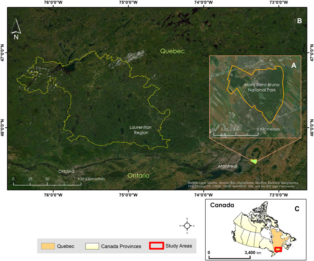
Figure 1. Two areas selected for the implementation of the phenospectral similarity metric: (A) Mont-Saint-Bruno National Park (MSB) classified under the sugar maple–bitternut hickory domain in Quebec and (B) ecoregion within the Laurentian region classified under the sugar maple–yellow birch domain. Panel (C) shows the approximate extent of the two study areas in relation to the province of Quebec and Canada.
2.2 Datasets
2.2.1 Satellite imagery
The analysis was conducted using multi-temporal imagery from both the PlanetScope Dove constellation (Dove PS) and Sentinel-2 (S2) satellite imagery (Table 1; Figure 2). These datasets were selected to determine the utility of their spatio-spectral and temporal resolutions for phenospectral similarity analysis. We selected relatively cloud-free (<10%) imagery for four dates covering the growing season from July to September. The Dove PS images have a 3-m spatial resolution and are comprised of four multispectral bands from the blue (465–515 nm), green (547–585 nm), red (650–680 nm), to near-infrared (845–885 nm) wavelengths (Planet Lab Inc, 2016). For the proof-of-concept at MSB, the imagery was downloaded as atmospherically compensated surface reflectance from the Planet Explorer data portal (Planet Lab Inc, 2021a). Clouds and shadows were masked followed by mosaicking of the individual image tiles in ENVI 5.5 (L3Harris Geospatial, Melbourne, FL). Similarly, relatively cloud-free S2 satellite images were downloaded from the USGS Earth Explorer directory (U.S. Geological Survey, 2021). The images were corrected from top-of-atmosphere (TOA: level 1 C) reflectance to bottom-of -atmosphere (BOA: level 2A) reflectance using Sen2Cor 2.2.1 (Müller-Wilm, 2016). Ten bands from S2 spanning from blue (band 2) to shortwave infrared (SWIR—band 12) were used for the analysis excluding the 60 m bands: band 1 (443 nm–coastal and aerosol), band 9 (940 nm), and band 10 (1,375 nm–cirrus). The bands with a 10 m pixel size were resampled to match the 20-m pixel size bands. Clouds were masked out of the S2 images using the scene classification file (SCL) generated from Sen2Cor. For the large-scale analysis, we utilized surface reflectance data from S2 and Dove PS imagery to compute PSpecM through the GEE platform. Due to a missing 2018 S2 image collection (i.e., surface reflectance) within GEE for the Laurentian region, the 2019 S2 image collection (surface reflectance product) was used for the large spatial scale analysis.
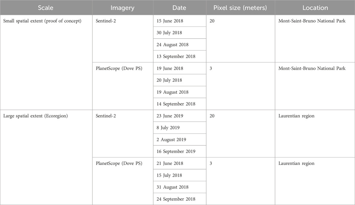
Table 1. Selected dates within the growing season and other characteristics of the PlanetScope Dove and Sentinel-2 satellite images used for the phenospectral similarity analysis.
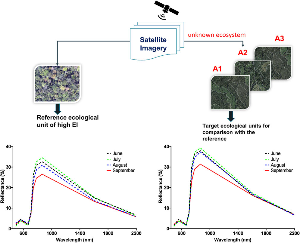
Figure 2. Comparison of the phenospectral changes of unknown ecological units (forest stands) and a reference forest stand of known high EI. A1 to A3 illustrates target ecological units (unknown forest stands) based on Sentinel–2 satellite imagery. The spectra presented represent the example spectra of a selected target ecological unit and a reference stand at MSB.
2.2.2 Selection of reference and target ecological units
The phenospectral similarity metric approach requires defining the target ecological units (forest stands with unknown EI) and a reference ecological unit that is known to be of high EI. As shown in Figure 2, a baseline or reference ecosystem known to be of high EI (see section 2.2.3) is compared to a set of target ecological units (i.e., unknown forest stands) within a broad ecological unit (e.g., Ecoregion). For MSB and the Laurentian region, 158 target polygons and ∼200,000 target polygons constituting different candidate stands (see section 2.2.4) were assessed in comparison to 1 and 14 reference ecological units, respectively. These reference data were selected from an exceptional forest ecosystem (i.e., “ancient” or old-growth forest) geospatial dataset produced by the province of Quebec (see section 2.2.3 for details).
2.2.3 Reference ecological units (exceptional forest ecosystem)
In the province of Quebec, Canada, the delineation of sites as exceptional forest ecosystems (EFEs) is done by the Ministry of Energy and Natural Resources (MRN). The EFEs are classified as rare forest, old-growth forest, or a forest that is a refuge (i.e., forests that serve as a home for threatened or endangered species) (Ministère des Forêts de la Faune et des Parcs, 2021b). An EFE is a special status designated by the MRN based on certain biophysical criteria. For instance, for old-growth forests (ancient or ancienne in French), EFE candidates must be forest stands without anthropogenic or major natural disturbance (Bouchard, 2005). The forest must be composed of very old trees and must be characterized by special features including, but not limited to, senescent and dead trees with the forest floor littered with large trunks in varying stages of decomposition (Ministère des Ressources naturelles, 2003c). Key quantitative definitions and criteria for the identification of old-growth forests in Quebec are described in detail by Villeneuve and Brisson (2003). Currently, a total of 256 sites have been delineated as EFEs across the province of Quebec, out of which 14 (old-growth forest category, see Supplementary Table S1) were in the Laurentian region (Ministry of Forests, 2016). Since the above definition of old-growth forest is consistent with the IUCN standard for sites delineated with respect to EI (IUCN, 2016), in this study, the old-growth forest (ancienne) polygons were deemed to have high EI and, hence, were utilized as the reference ecological units to serve as inputs for PSpecM implementation, as described in 2.2.2 above.
2.2.4 Target ecological units from the eco-forestry inventory (peuplements forestiers)
Over half of the province of Quebec’s territory is forested (i.e., ∼900,000 km2) (Ministère des Forêts de la Faune et des Parcs, 2016). Forest inventories over the years have been focused on ecological and dendrometric data (e.g., ecological classifications and tree height (LiDAR)) to allow delineation of forest cover, disturbed areas, and others that make up the Quebec forest landscape (e.g., Southern Quebec eco-forest inventory—IEQM) (Ministère Des Forêts De La Faune et Des Parcs, 2021a). In this study, publicly accessible forest inventory data (peuplements forestiers) provided by the Ministry of Forest, Wildlife, and Parks (Ministry of Forests, 2021), which provides information on the management and sustainable development of forest ecosystems in Quebec, were used. The forest inventory data were used as candidate stands (target ecological units) to identify potential ones of high EI, as required in section 2.2.2. The median area of the peuplement forestier layer (i.e., unknown ecological units) covering our study area is approximately 4 ha, and the land cover type of each target polygon falls within either the deciduous stand (F) (49.84%), mixed stands (M) (30.16%), or softwood (R) and other (not defined) category (20%).
2.3 Computation of the phenospectral similarity metric (PSpecM)
The mean reflectance of each target ecological unit (peuplement forestier polygon) was computed for each time period (Table 1). The spectral angle (Eq. (1)) was then computed between the reference and the target ecological units separately for each temporal data, and the spectral angles were also averaged across all dates within the growing season. The spectral angle has been commonly applied to image classification, target detection, and related questions (Kumar et al., 2015; Panda and Pradhan, 2015). The algorithm computes the “angle” in the multi-dimensional space between a target and reference spectrum by treating them as vectors in space with dimensionality, which is equal to the number of bands (Kruse et al., 1992; Yuhas et al., 1992; Kruse et al., 1993; Rashmi et al., 2014). The computed spectral angle thus serves as a quantitative measure of the similarity between the target and reference spectra. The spectral angle computed using reflectance data is relatively robust to illumination and albedo effects (Kruse et al., 1993).
The spectral angle (α) between a reference (r) and a target (t) spectrum is computed according to Equation 1 as follows:
where nb represents the number of bands.
2.3.1 Determining the spectral angle threshold
The real value–area fractal technique (Shahriari et al., 2014) was adopted to determine a suitable spectral angle threshold for delineating stands with high EI. This method has been shown to be a less biased approach for determining thresholds for applications such as density slicing and image classification/segmentation (Shahriari et al., 2014). Equation 2 is used to establish a power–law relationship between an area (A: number of polygons (target ecological units) with a spectral angle (α) above a certain threshold (s)).
where A(α) represents the area occupied by the target polygons with a spectral angle greater than or equal to a particular threshold (s) and b represents the fractal dimension.
By plotting a log–log of A(α) versus α, segments or straight lines are typically derived, with each segment corresponding to a group of spectral angles less than or equal to a particular threshold. To determine a spectral angle threshold from the log–log plot, an intersection of the segments/lines is selected, and the corresponding value on the X-axis is extracted. The threshold is then computed by taking the exponent of the extracted value to help with delineating polygons with high EI. The intersection of the second segment has been recommended for the computation of the threshold value for each temporal data and the average spectral angles across the growing season (Shahriari et al., 2014).
2.4 Google Earth Engine
Google Earth Engine (GEE) provides a cloud-based platform and tools for planetary scale analysis, making satellite imagery spanning about 4 decades available (Gorelick et al., 2017; Amani et al., 2020). Through GEE, the methodology can be reproduced at multiple scales and shared with multiple users. In this study, scaling the analysis to a large spatial scale (ecoregion) was undertaken on the internet-accessible GEE environment that is programmable using JavaScript (Gorelick et al., 2017).
2.4.1 Spatial aggregation of the target ecological units based on the proximity to a reference
At the large spatial scale, a spatial aggregation of the target ecological units based on their proximity to a reference stand of high EI was carried out (Supplementary Figure S9). Assigning the target ecological unit to the closest reference site was deemed an appropriate stratification approach since nearer stands of the same land cover type will be more related than the distant stands (Pun-Cheng, 2016; Waters, 2018), and it also helps reduce temporal lag in phenological activity due to latitudinal or altitudinal variations. The 14-reference ecological unit from the EFE (old-growth forest) layer was split into two, and seven reference polygons served as a representative reference distribution to be compared to approximately 200,000 target ecological units across the study area in the Laurentian region, Quebec. The remaining seven were added to the large target ecological units to test the PSpecM method. Next, to aggregate the large set of target ecological units, a spatial proximity analysis was conducted in ArcGIS 10.7.1 (Esri, Redlands, CA, United States, 2019) to determine which reference polygon is nearest to a target polygon.
In this study, filtering of the target ecological units (peuplements forestiers) was done to exclude water bodies. Additionally, after the implementation of PSpecM, we compared the environmental conditions (e.g., drainage and surface deposits), age, and terrain types of the delineated polygons to that of the reference sites. Supplementary Table S2 presents the key environmental characteristics of the reference sites, as determined by superposing the seven reference polygons on the eco-forest classification (peuplements forestiers) in Quebec (Ministère Des Forêts De La Faune et Des Parcs, 2021a).
2.4.2 Scaling the implementation of phenospectral similarity in Google Earth Engine
To evaluate the scalability of the PSpecM at the ecoregion scale, the image collections (Table 1) were imported and mosaicked in GEE. Next, the cloud/shadow mask was applied (Justin, 2022), and the mosaics were clipped to the extent of the study area. Subsequently, we applied the mean reducer in GEE to extract the mean spectrum for each target and the corresponding reference polygon. The extracted means were used to compute the spectral angle between each target and the corresponding reference ecological unit. The computed value is then assigned to each record in the target ecological unit layer, and a threshold is applied (section 2.3.1.) to identify the potential areas of high EI. Figure 3 illustrates the flow chart summarizing the PSpecM workflow in GEE.
Figure 3. Flow chart summarizing the workflow to be followed during the implementation of PSpecM in Google Earth Engine (GEE).
To assess the robustness of PSpecM, a time sequence analysis was conducted at MSB using S2 surface reflectance available in GEE for the years 2019, 2020, and 2021 (Table 2). Missing datasets in June for the selected years were replaced with S2 imagery acquired in May.
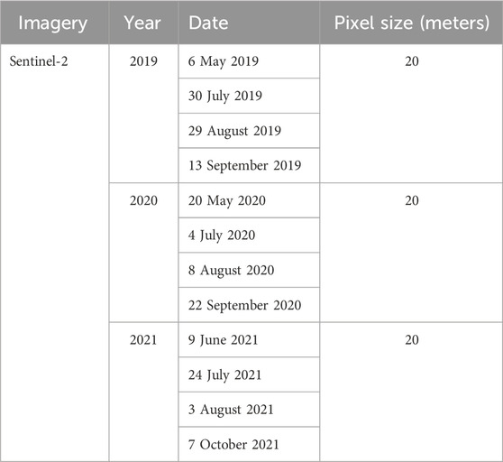
Table 2. Selected dates for Sentinel-2 satellite imagery used for time series analysis to assess the robustness of the phenospectral similarity analysis at the Mont-Saint-Bruno National Park site.
3 Results
3.1 Comparison of phenospectral changes from Sentinel-2 and PS dove of the reference forest stand (Mont-Saint-Bruno proof of concept)
Figures 4A and B show the mean reflectance spectra and reflectance differences extracted from PS Dove imagery for the reference forest (MSB) throughout the growing season. The chlorophyll absorption in the blue and red bands decreased gradually from the start (June) to the end of the growing season (September). However, the differences recorded were negligible, for example, approximately 0.3% and 0.1% for the blue and the red bands, respectively. Similarly, the reflectance in the green band recorded at the beginning of the growing season reduced slightly by a similar amount to that in the red band in the month of September. Considering the Dove PS imagery, the highest changes in the mean reflectance were recorded in the near-infrared band, which decreased from 44.3% to 33.7% (i.e., 10.6%) at the end of the growing season.
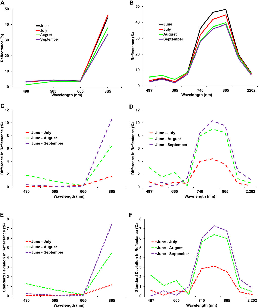
Figure 4. (A) Mean reflectance spectra extracted from Dove PS across the growing season (June–September). (B) Mean reflectance spectra extracted from Sentinel-2 imagery for the reference forest at Mont-Saint-Bruno National Park throughout the growing season (June–September). (C) Differences in Dove PS reflectance between June and the months of July, August, and September. (D) Differences in Sentinel-2 reflectance between June and the months of July, August, and September. (E) Standard deviation between June and the months of July, August, and September of Dove PS imagery. (F) Standard deviation between June and the months of July, August, and September of Sentinel-2 imagery.
The mean reflectance of the reference forest throughout the growing season, along with their differences extracted from the S2 satellite imagery and standard deviation, is presented in Figures 4C–F. The reflectance recorded at the beginning of the growing season for the blue and red bands increased slightly by approximately 3% and 2%, respectively, by August and started to decline further by a similar amount in September. Additionally, the reflectance in the green band increased up to 1.5% in August and decreased by 2.3% during the end of the growing season in September. The bands covering the red-edge portions of the electromagnetic spectrum exhibited a steady decline in reflectance from June to September. Lastly, the SWIR bands recorded a decrease in the mean reflectance of up to 2.5% between June and September (Figures 4C, D).
3.2 Single-year spectral angle from Mont-Saint-Bruno (proof of concept)
The summary of the 90th percentile range of the spectral angles computed using reflectance from Dove PS Imagery for the target ecological units is presented in Figure 5A. At the beginning of the growing season in June (2018), an average spectral angle of 0.025 ± 0.031 (minimum: 0.0007 and maximum: 0.164) was determined for the selected forest stands at MSB. Subsequently, the average spectral angle slightly increased between July (0.026 ± 0.036) and August (0.022 ± 0.025). The maximum of 0.173 and 0.121 and the minimum of 0.0008 and 0.0003 spectral angles were recorded for July and August, respectively. In September, the mean spectral angle was 0.029 ± 0.032, while the minimum and maximum were 0.0009 and 0.131, respectively. The mean spectral angle recorded across the growing season for the Dove PS imagery was 0.026, while the threshold value was determined to be 0.014. When this threshold is applied, 79 (796.6 ha) target ecological units out of a total of 158 polygons were determined to be phenospectrally similar to the baseline polygon for the Dove PS imagery (Figure 6). In comparison, when separate thresholds are applied to each temporal data across the growing season, 54 polygons (581 ha) were selected for PS Dove imagery. Table 3 shows the number of polygons and the thresholds applied to each temporal data including the mean spectral angles using PS Dove imagery.
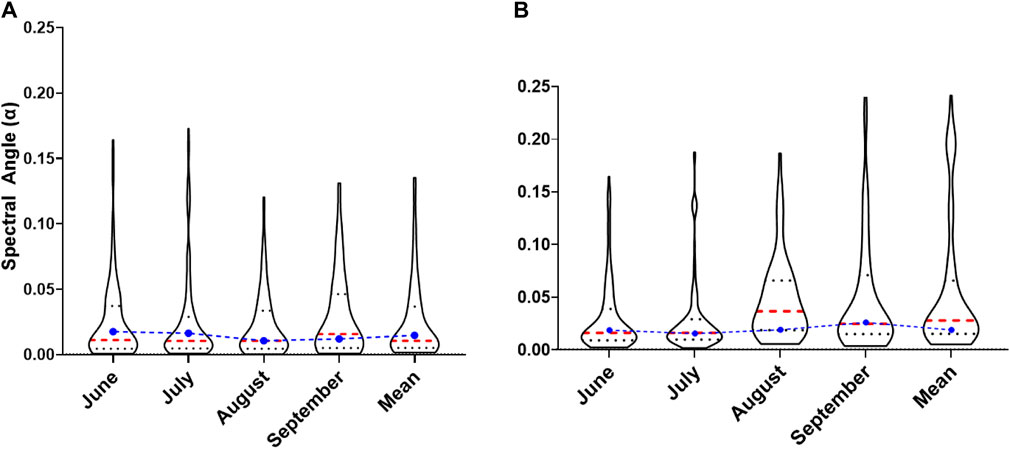
Figure 5. Violin plot of the 90th percentile range of the spectral angle for MSB (June–September 2018 and the mean) computed across the growing season and the mean over the entire temporal period from (A) PS Dove and (B) Sentinel-2 Satellite. The red dashed lines represent the median, whereas the dark dotted line represents quartiles. The blue dot and dashed lines show the threshold for the mean spectral angles across the growing season in radians.
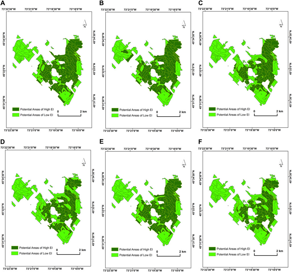
Figure 6. Spatial distribution of the selected potential areas of high EI from PlanetScope (Dove) imagery at MSB (A) June image (α < 0.0169), (B) July image (α < 0.0157), (C) August image (α < 0.0099), (D) September image (α < 0.0113), (E) mean (α < 0.0141), and (F) polygons that are consistently selected across the selected dates in the growing season. The acquisition dates of the PS Dove images used for the PSpecM analysis falls within the growing season (June–September 2018).
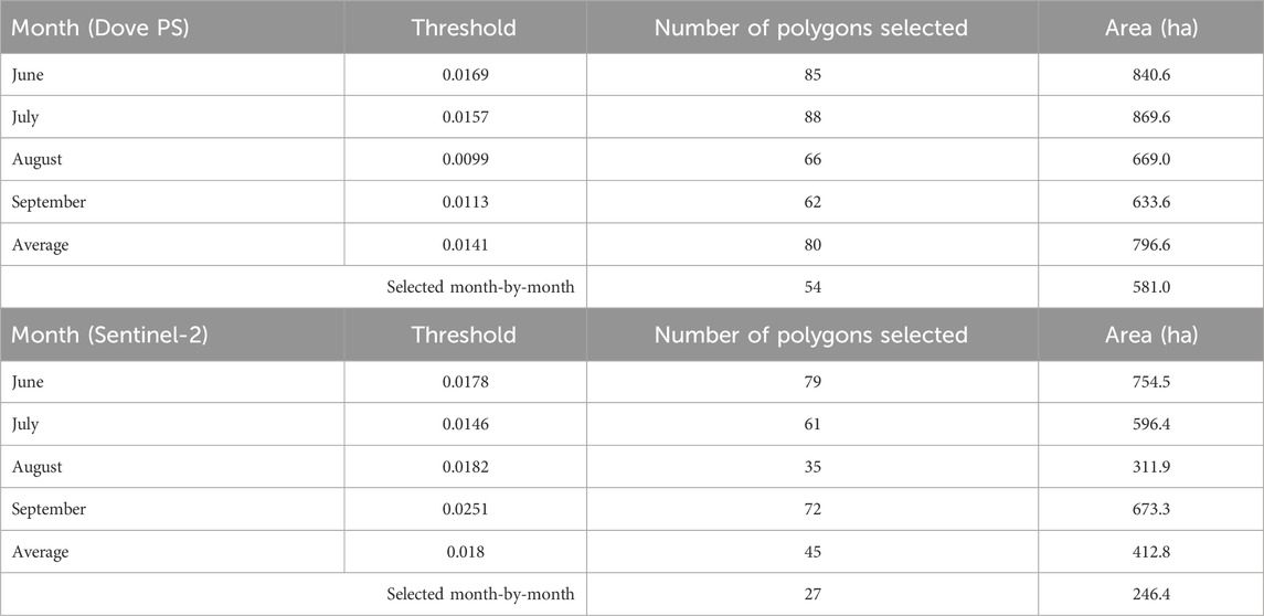
Table 3. Number of selected polygons and spectral angle thresholds determined for each temporal data and that of the mean spectral angle at the Mont-Saint-Bruno National Park site using PS Dove imagery and Sentinel-2 satellite imagery.
Furthermore, the mean spectral angle computed for S2 imagery at the beginning of the growing season in June (0.031 ± 0.034) and July (0.029 ± 0.035) was lower compared to that in August (0.048 ± 0.039) and September (0.061 ± 0.0.084). An average of 0.056 ± 0.063 was recorded for the June–September period (Figure 5B). Additionally, for the S2 data, the threshold for the mean spectral angle recorded was 0.018 (Figure 5B). Based on this mean spectral angle threshold, 45 target ecological units (412.8 ha) were found to be phenospectrally similar to the reference condition when S2 data are used for the analysis (Table 3). However, the application of separate thresholds month-by-month resulted in the selection of 27 polygons (246.4 ha) as potential areas of high EI. Table 3 and Figure 7 present the thresholds determined for each temporal dataset, the spatial distribution of the selected polygons, and number of areas delineated as potential areas of high EI.
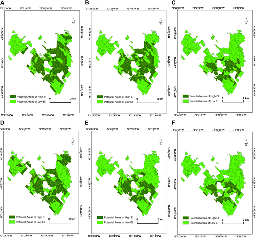
Figure 7. Spatial distribution of selected potential areas of high EI from Sentinel-2 imagery at MSB: (A) June image (α < 0.0169), (B) July image (α < 0.0157), (C) August image (α < 0.0099), (D) September image (α < 0.0113), (E) mean (α < 0.0141), and (F) polygons that are consistently selected across the selected dates in the growing season. The acquisition dates of the Sentinel-2 images used for the PSpecM analysis falls within the growing season (June–September 2018). These dates are presented in Table 1.
3.3 Assessment of PSpecM robustness for the delineation of potential areas of high EI (multi-year)
3.3.1 Mean spectral angle
For the time sequence analysis at MSB, the proportion of sites delineated as potential areas of high EI when the mean spectral angle across the selected dates is used for 2019 was 41 target ecological units (429.7 ha) (Figure 8A). Furthermore, for 2020 and 2021, the delineated stands reduced slightly to 35 (374.6 ha) and 36 (386.78 ha) target ecological units, respectively (Figures 8B and C). A year-on-year (2019–2021) comparison of the proportions of areas determined to be of potentially high EI shows that the 2019–2020-year range recorded the lowest temporal variability. The year 2019–2020 recorded the highest number of commonly delineated polygons (33 target ecological units, 347.55 ha), followed by 2019–2021 (31 target ecological units, 352.58 ha), with the highest temporal variability (17 ecological units delineated, 204.70 ha) recorded between 2020 and 2021. Eight ecological units constituting 111 ha were delineated three times across the 3 years’ time sequence analysis (Figures 8A, B, and D).
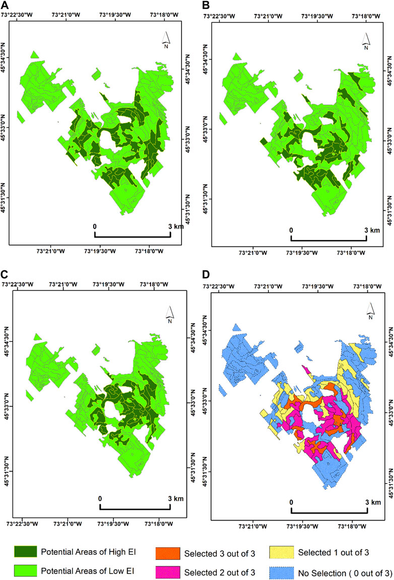
Figure 8. Time sequence PSpecM analysis using Sentinel-2 satellite imagery acquired between (A) 2019 (mean spectral angle threshold (α) = 0.0283), (B) 2020 (mean spectral angle threshold (α) = 0.0184), and (C) 2021 (mean spectral angle threshold (α) = 0.0324). (D) Map showing the number of times the ecological units or target polygons were selected across the years. This analysis uses the mean spectral angle across the growing season.
3.3.2 Multi-year analysis accounting for seasonal variation in spectral reflectance
The results when separate spectral angle thresholds are applied to each temporal data for the time sequence analysis at MSB are presented as follows; for 2019, the PSpecM analysis at MSB identified 31 target ecological units (356.76 ha) as potential areas of high EI (Figure 9A). In 2020, the delineated target ecological units increased slightly to 36 polygons (379.92) (Figure 9B). Additionally, the delineated stands were somewhat lowered for 2021 as 18 polygons (386.78 ha) were identified as potential areas of high EI (Figure 9C). A year-on-year (2019–2021) comparison of the areas found to potentially have high EI for the chosen years are presented as follows. The lowest temporal variability was found in the 2019–2020 year range accounting for twelve identified polygons, whereas the highest temporal variability (eight ecological units delineated) was found in the 2-year interval between 2019 and 2021. Five ecological target ecological units (70.42 ha) were identified by the PSpecM analysis across the selected years (Figure 9D) in comparison to eight units when the growing season average threshold was used (Figure 8D).
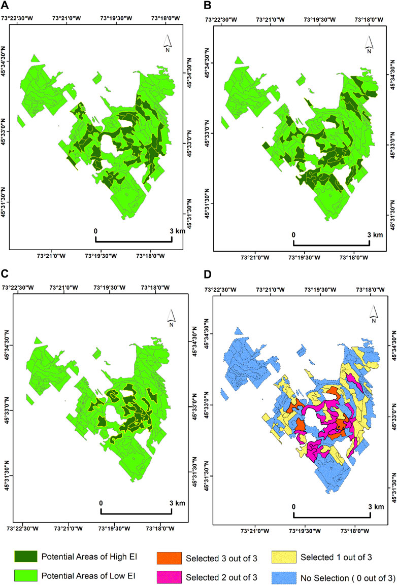
Figure 9. Time sequence PSpecM analysis using Sentinel-2 satellite imagery acquired between (A) 2019 (May threshold (α) = 0.0215, July threshold (α) = 0.0286, August threshold (α) = 0.0237, and September threshold (α) = 0.0343), (B) 2020 (May threshold (α) = 0.0266, July threshold (α) = 0.0332, August threshold (α) = 0.0353, and September threshold (α) = 0.0313), and (C) 2021 (June threshold (α) = 0.0323, July threshold (α) = 0.0270, August threshold (α) = 0.0260, and October threshold (α) = 0.0323). (D) Map showing the number of times the ecological units or target polygons were selected across the years.
3.4 Identification of potential areas of high EI over large spatial extents in Google Earth Engine
The maps in Supplementary Figures S1–S4 illustrate the variability of spectral angles calculated for each unknown ecological unit across the growing season and the corresponding multitemporal images from both sensors. Considering Dove PS imagery, the computation of the average spectral angle across the growing season resulted in a mean (0.033 ± 0.039) and a minimum and maximum spectral angle of 0.00009 and 0.762, respectively. The threshold value calculated for the Dove PS imagery at the ecoregion scale for selected months within the year and the mean are presented in Table 4 and Supplementary Figure S5. When these thresholds are applied to each temporal data and their average spectral angles (Supplementary Figure S5F), 112,483 (6,397.1 km2) and 65,172 (3722.84 km2) target ecological units, respectively, were found to be phenospectrally similar to the reference polygons, which constitutes 30% and 52% of the total area, respectively (Supplementary Figure S5E). Moreover, for the S2 imagery analysis at the large spatial scale, after averaging the spectral angles across the growing season, the minimum and maximum spectral angles for S2 were 0.003 and 1.03, respectively, and a mean of (0.043 ± 0.052). The threshold value as determined for S2 for all months and the mean spectral angles are presented in Table 4. Based on these thresholds, using the mean spectral angle data, 121,370 polygons (7,128.4 km2) equivalent to 58% of the total area were identified to be phenospectrally similar to the reference stands. When the thresholds are applied month-by-month to account for seasonal variation in reflectance, 95,996 target ecological units were identified by PSpecM as potential areas of high EI, which also constitute 46% of the total area of the study site (Supplementary Figure S6). Comparing both PS Dove and S2 results, for the mean data, approximately 94,691 ecological units corresponding to a total area of 55,005 km2 were delineated by both sensors (Figure 10A). However, 47,222 (2,773.55 km2) polygons equivalent to 22.5% of the total area were identified by a multi-year comparison of S2 and the Dove PS data that account for the phenological effect on reflectance (Figure 10B).
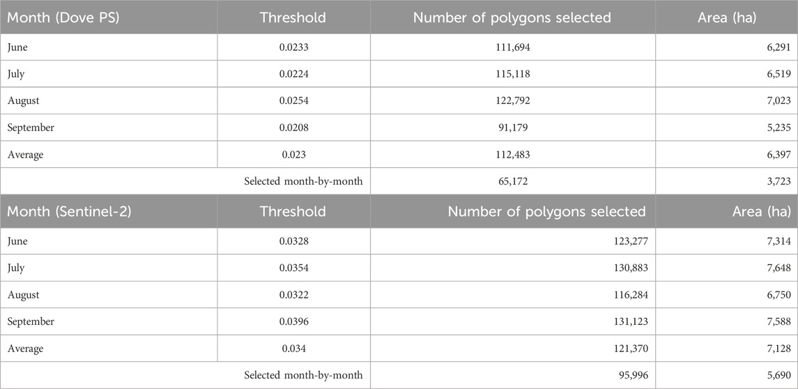
Table 4. Number of selected polygons and spectral angle thresholds determined for each temporal data and that of the mean spectral angle at the large spatial scale (ecoregion) using Dove PS satellite imagery and Sentinel-2 satellite imagery.
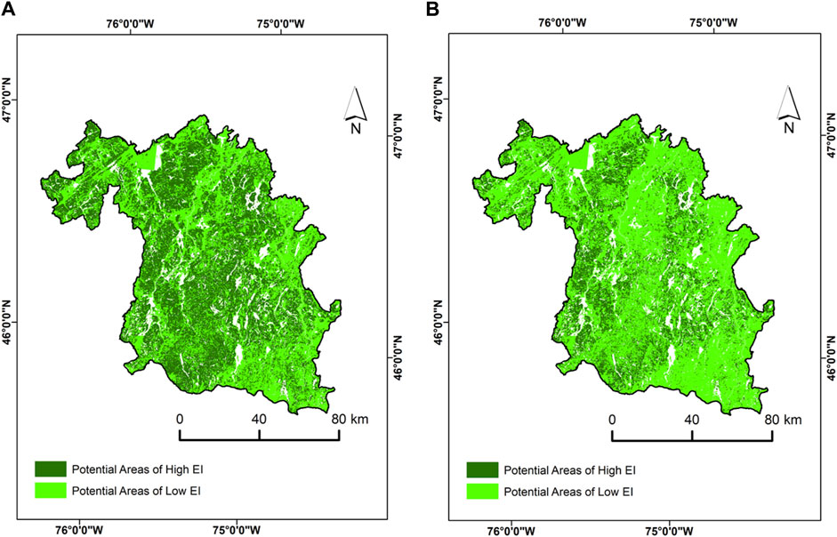
Figure 10. Spatial distribution of potential areas of high EI (deep green) delineated using multi-year satellite imagery (i.e., both Sentinel-2 and PlanetScope (Dove) satellite imagery). (A) Multi-year delineated polygons by averaging spectral angles across the growing season; (B) multi-year reduced delineated polygons when individual thresholds are applied on a month-by-month basis for each year to account for the phenological cycle effect across the growing season. The acquisition dates of the Sentinel-2 and PS Dove images used for the PSpecM analysis falls within the growing season (June–September 2018 and 2019). These dates are presented in Table 1.
3.5 Testing of identified potential areas of high EI with the reference polygons
The results obtained using the testing reference sets described in 2.4.1 are presented in Supplementary Figure S8. For both sensors, Baie Amélia differed the most, recording an average spectral angle of 0.045 (Dove PS) and 0.035 (S2). Conversely, Lac-Saint-Paul and Lac Gagnon were phenospectrally similar to the reference polygons recording the spectral angle range of 0.004–0.008 for Dove PS and 0.013–0.014 for S2 (Figure 11). Overall, when individual thresholds are applied to each temporal data to account for the phenological effect at the ecoregion scale, five of seven (71.4%) were identified as potential areas of high EI for both sensors. Meanwhile, the use of means spectral data produced six out seven (85.7%) testing polygons identified as areas of high EI in the case of Dove PS, while five out seven (71.4) were selected for S2 imagery. The S2 spectral angle range representative of the target ecological units delineated as potentially low EI areas varied between 0.039 and 1, with a mean spectral angle of 0.06 larger than the remaining categories (Figure 11). The mean spectral angle for potential high EI areas (both multi-year and single year) ranged between 0.010 and 0.018, while the mean spectral angle for the testing polygons delineated as potential high EI areas (multi-year) was 0.014.
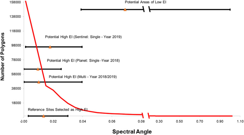
Figure 11. Comparison of PSpecM results for single-year and multi-year (2018/2019) analyses with the testing sets. The red curve illustrates the statistics of the target ecological units and spectral angle with statistics for distinct categories, including the reference sites (potential areas of low and high EI (multi–year) and potential areas of high EI for single year). Potential areas of high EI (multi-year) constitute areas selected by both sensors (PlanetScope (Dove) and Sentinel-2) in 2018/2019. The triangles are the mean, and the ends of the whiskers are the maximum and minimum spectral angles for their respective category.
3.6 Comparison of the land cover type and environmental conditions of the reference sites versus the identified potential areas of high EI
For both sensors and taking into consideration the phenological effect, out of the over 47,222 commonly delineated target ecological units as potential areas of high EI, 93.2% were classified with surface deposit types consistent with that of the reference sites (1AY, 1A, 1AM, or R1A) (Supplementary Figure S7). Additionally, as shown in Supplementary Table S2, the potential areas of high EI identified had a similar drainage classification range (classes 10, 20, 30, 31, and 40) as the reference sites. This suggests that if a reference used for comparison had a drainage class of 10, then the corresponding areas of high EI will also have a class of 10. Moreover, the predominant age class identified for S2 delineated potential areas of high EI were old uneven stand, young uneven stand, and an old irregular stand (>80 years) classifications, which is also consistent with that of the reference sites. All the delineated potential high EI stands are classified under the land category of the terrain type. Finally, 98% of the delineated polygons of high EI can be categorized under deciduous and mixed stand land cover types, which is consistent with that of the reference sites.
4 Discussion
In this study, we have shown the use and implementation of a phenospectral similarity metric (PSpecM) as an index of EI for identifying potential areas of high EI over a large spatial scale to prioritize them for conservation interventions. To the best of our knowledge, our study represents the first attempt to utilize a PSpecM to delineate potential stand level areas of high EI. Moreover, our study did so at a large geographic scale via Google Earth Engine’s geospatial analysis platform to complement the existing conservation tools and potentially support the ongoing KBAs initiative. It is important to highlight that our proposed approach, PSpecM, provides a way of estimating EI and not a way to determine the location and extent of KBAs. However, the results from PSpecM implementation could be useful in the determination of KBAs.
Our analysis shows that the utilization of forest canopy spectral changes across the growing season (phenospectral) highlights the spectral–temporal dynamics (Figure 4) to aid in large-scale identification of potential areas of high EI at the stand level. The PSpecM approach is sensitive to the canopy phenological characteristics, composition, and biophysical and structural attributes of the delineated potential high EI forest stands. In the forest zone of southern Quebec, Canada, these attributes form part of the key considerations for classifying sites as exceptional forest ecosystems (Villeneuve and Brisson, 2003). Thus, the usefulness of PSpecM in narrowing the potential areas of high biodiversity and the opportunity to monitor periodic changes of their extent can be explored further to support the province’s biodiversity management efforts. Additionally, in Canada, the identification of key biodiversity areas with respect to EI (criterion C) has been deferred pending the development of methods to identify KBAs for Canada (KBA Canada Coalition, 2021). Criterion-C KBA sites are large areas (>10,000 km2), with one or two expected per ecoregion across the globe. Due to the scalable nature of our approach, successful implementation of this metric at the ecoregion scale in Quebec is a good indication that PSpecM can be refined to complement the existing tools (Beyer et al., 2020) for large-scale monitoring and prioritization of high EI areas.
For a candidate stand that is phenospectrally similar to a reference forest, a smaller spectral angle is expected to serve as a quantitative measure of spectral similarity of that ecological unit to the reference site. Over the years, utilization of the spectral angle as a mapping approach has been shown to be robust, and it provides better classification and target detection outcomes compared to traditional classifiers (Sohn and Rebello, 2002). Our results for the time series analysis show that, although there were some uncertainties in the delineated areas of high EI, a considerable number of target ecological units were consistently delineated as areas of high EI across the selected years (Figures 8 and 9) when either the mean spectral angle is used or when separate thresholds are applied month-by-month to account for phenological effects.
Phenology is closely related to biodiversity and ecosystem dynamics. Therefore, it is important, when possible, to consider the effect of phenological cycles on the spectral variation in forest canopies (phenospectral) by analyzing the imagery on a month-by-month basis throughout the growing season. From Figures 8D and 9D, yellow polygons will normally not be selected as candidates because they were only selected in 1 year. Ideally polygons selected 3/3 times will be considered candidate stands of high EI, and special consideration will be given for the ones selected twice before inclusion. The temporal consistency observed in the time sequence analysis is a good indication of the usefulness of the PSpecM approach for rapid delineation of potential high EI areas. The observed temporal variation in the delineated stands of high EI can be improved by exploring different spectral angle thresholds. Additionally, temporal changes in vegetation dynamics (e.g., deforestation) and image contamination by clouds and shadows could also explain the differences in the delineated stands (temporal variation) observed across the selected years.
To detect candidate stands of high EI over a large geographic extent (i.e., from ecoregion to national to global scales), the use of GEE for the implementation of the PSpecM is recommended for an optimized workflow. GEE serves as an effective online environment to extract and integrate either freely available (e.g., Sentinel-2 and Landsat) or access-restricted (e.g., Planet data) multitemporal imagery into a complex analytical workflow (Tassi and Vizzari, 2020). As demonstrated in this study, by implementing PSpecM in GEE, the workflow (described in Section 2.2.1) decreased in part because most of the preprocessing steps such as atmospheric correction had already been applied to the S2 imagery in the catalog. With these available images, implementation of the PSpecM would be straightforward, following filtering of the image collections. The entire computation can be automated programmatically using JavaScript, thus permitting the repetition and reproduction of the workflow on different image collections (Gorelick et al., 2017). At the national or global scale, manual download and implementation of the analytical methods (described under Section 2.2.1) can be a daunting and time-consuming task due to the high volume (e.g., ecoregion scale: ∼40 GB) of satellite imagery and the requirement of computing capacity for such an amount of data. These constraints can be overcome by adopting the GEE platform, which serves as a catalog of satellite imagery and other geospatial datasets with global coverage (Gorelick et al., 2017; Amani et al., 2020; Hu et al., 2020) and provides digital processing capacity to reduce the amount of time needed to analyze such large datasets locally (Daldegan et al., 2019). Unlike the proof-of-concept analysis (MSB), in GEE, there is no need to manually download and process individual tiles locally (Daldegan et al., 2019). Juxtaposing these benefits with promising results from previous research (Tracewski et al., 2016; Beresford et al., 2020) and the focus of ongoing conservation projects such as the Cambridge Conservation Initiative (2019), it is inevitable that soon, GEE will be widely adopted by conservationists across the globe for large-scale KBA identification and assessments.
Comparing the results from the Dove PS imagery to that of S2 satellite imagery at a small spatial scale, the extent of the forests identified as high EI reduced (e.g., from 54 to 27 polygons at MSB) with imagery with a greater spectral resolution (Figures 9A and B). The Dove PS imagery has the advantage of high spatial resolution (3 m) at the expense of spectral resolution (4-bands), while S2 has a coarser spatial resolution (20 m) but a higher spectral resolution in comparison (Planet Lab Inc, 2016; Radoux et al., 2016). In both multi-spectra datasets, in the visible bands, the spectral characteristic of vegetation is similar since the vegetation exhibits photosynthetic absorption in the blue and red wavelengths and higher reflectance in the green region of the electromagnetic spectrum (Gates et al., 1965). Additionally, the most common applications of the coarse spectral resolution of Dove PS imagery have been for mapping the temporal phenology and tracking of small-scale ephemeral forest cover dynamics (Pickering et al., 2021). This implies that undisturbed stands (irrespective of species composition difference compared to a reference site) could be captured as potential areas of high EI, which explains why more target ecological units were identified to be of high EI when Dove PS Imagery was used for the analysis. However, with S2, there are additional spectral bands in the red-edge, near-infrared (NIR), and shortwave infrared (SWIR) (Radoux et al., 2016). These bands help maximize species-specific differences (Grabska et al., 2019) and highlight canopy leaf structural and biochemical compositions (chlorophyll and water content) (Brown et al., 2019). Additionally, for a sub-canopy pixel size, it is possible to observe the spatio-temporal variability induced by external factors, such as shading at separate times of the year. These factors could explain why the number of stands identified to be of high EI for S2 imagery differed from that of Dove PS.
From Supplementary Figure S7, it can be deduced that the environmental conditions (e.g., surface deposits and drainage) of the delineated potential stands of high EI were similar to that of the reference ecological units. Less than 6% of the delineated stands of high EI had different surface deposit types compared to the reference sites (Supplementary Figure S7). This suggests that the environmental conditions of the reference sites could play a key role in the selection of potential sites of high EI. In this study, filtering of the target units in terms of environmental conditions was not included in the workflow prior to PSpecM implementation. As a result, phenospectral dissimilarity of a candidate stand may not necessarily imply that a site has low EI but could constitute differences in the environmental conditions. For instance, non-filtering of target polygons based on the similarity of land cover type and environmental conditions as reference sites (e.g., peatland vs. peatland and forest vs. forest) could result in the delineation of an undisturbed forested peatland as having low EI relative to an old-growth mesic reference forest on well-drained soil. Although both sites may have high EI, phenospectral dissimilarity could be observed because of the compositional and structural differences caused by their respective environmental conditions (Mosseler et al., 2003; Andersen et al., 2011).
For both multispectral datasets, the Baie Amélia reference site differed most from the reference polygon (Lac Cuillèrier) used for the comparison. Although Baie Amélia and Lac Cuillèrier exhibit similarity in terms of species composition (e.g., both sites have sugar maple and yellow birch trees), they differ with respect to topographic complexity (Ministère des Ressources naturelles, 2003a, ministère des Ressources naturelles, 2003b). The reference site Lac Cuillèrier is characterized by gentle to moderate slopes (relatively less rugged terrain), whereas Baie Amélia is characterized by rugged relief (Ministère des Ressources naturelles, 2003a, ministère des Ressources naturelles, 2003b). Phenological variations (phenospectral) are typically driven by topographic, edaphic, and climatic factors of a unit area (Cho et al., 2010). Topographic effects result in substantial shadowing to cause variable canopy reflectance values (Nath and Ni-Meister, 2021). Apart from the topographic complexity (such as slope, elevation, and aspect), structural complexity resulting from variations in tree height and rugosity can also influence the spectral reflectance measured at the forest canopy (Nath and Ni-Meister, 2021). These dynamics could explain the phenospectral dissimilarity observed with regards to the reference (Lac Cuillèrier) and testing (Baie Amélia) polygons.
The key challenge in the implementation of the phenospectral similarity metric on a large spatial scale is limited data for the reference sites (key limitation), spatiotemporal satellite data acquisition throughout the growing season, and the availability of cloud-free satellite imagery. Cloud, shadow, and haze contamination compromise the usability of satellite imagery. Although the JavaScript functions developed incorporates cloud and shadow removal for S2 imagery (Justin, 2022), clouds and shadows are generally difficult to eliminate; thus, remaining clouds may contribute to incorrect estimates of PSpecM for the affected stand. In cases with an extensive cloud cover, a combination of available cloud-free multi-temporal data from multiple spaceborne sensors should be explored and utilized for the PSpecM analysis. Additionally, the target ecological units employed in the PSpecM analysis are accessible as file geodatabase and ESRI shapefile formats, with only the latter currently supported in GEE. However, the ESRI shapefile format has a size limit of 2 GB (ESRI, 2021); hence, the target ecological units from which to select candidate stands of high EI cannot exceed this limit unless a different format or multiple shapefiles are used.
It is important to note that, in temperate climate, since most trees in deciduous forest lose their foliage at the end of the growing season, there is a limited window (i.e., during the growing season), for which this methodology would be appropriate. Future studies should consider including the leaf senescence period where many deciduous tree species change color to assess the usefulness of those periods for delineating stands of high EI. Moreover, for other forest types (e.g., evergreen), multitemporal data across different seasons could be explored to determine the appropriate image dates for PSpecM analysis. Additionally, considering that forest stands exhibit similar spectral characteristics (especially in the visible and near-infrared range for Dove PS and Sentinel-2) during the growing season, future studies could explore the use of a greater number of temporal images (not only four) to reduce temporal uncertainties.
5 Conclusion
Using Sentinel-2 and PlanetScope (Dove PS) satellite imagery, we have illustrated at two spatial scales the usefulness of the phenospectral (reflectance changes across the growing season) similarity metric in identifying potential sites of high EI. Phenospectral similarity can be associated with species composition and phenological, structural, and functional biodiversity of the forest canopy to enable the delineation of stand-level potential areas of high EI over large spatial scales (i.e., thousands of km2).
The main benefit of our approach is in its ability to integrate taxonomic, phylogenetic diversity, and structural aspects of vegetation that are important for EI at the stand level. Hence, PSpecM can serve as an important first step to narrow down important biodiversity areas at broader geographic scales using Earth observation satellite data. Due to the scalable nature of the PSpecM, it is expected that our approach will contribute to measuring EI that can potentially be applied to KBAs identification at multiple spatial scales. The key limitation of our approach is the availability of reference sites of known high EI to act as reference ecological states. The implementation of PSpecM requires a reference stand known to be of high EI and unknown target ecological units of the same land cover type and environmental conditions (e.g., drainage and surface deposits) for comparison to delineate potential areas of high EI. As Canada leads the implementation of new and systematic approaches to identify KBAs, our approach could potentially serve as a novel complementary conservation tool to contribute to KBA identification (i.e., the EI criterion could be measured using our approach, which could lead to an improved outcome) countrywide and potentially at the global scale.
Data availability statement
The original contributions presented in the study are included in the article/Supplementary Material; further inquiries can be directed to the corresponding author.
Author contributions
PO: conceptualization, data curation, formal analysis, methodology, software, validation, writing–original draft, and writing–review and editing. EL: conceptualization, funding acquisition, methodology, validation, and writing–review and editing. MK: conceptualization, methodology, supervision, and writing–review and editing. JA-M: methodology, supervision, and writing–review and editing. AG: conceptualization, funding acquisition, methodology, and writing–review and editing. JZ: conceptualization, methodology, and writing–review and editing.
Funding
The author(s) declare that financial support was received for the research, authorship, and/or publication of this article. This research was supported by MITACS and the Natural Sciences and Engineering Research Council of Canada through the Canadian Biodiversity Observatory (CABO). The Department of Geography, McGill University, provided access to PlanetScope (Dove) imagery. Authors JZ and AG further thank the Liber Ero Chair in Biodiversity Conservation for funding.
Acknowledgments
Author POD thanks Dr. Deep Inamdar of the Applied Remote Sensing Lab (ARSL), McGill University and Mr. Facundo Smufer (Université du Québec à Montréal (UQAM), for discussions on the methodology.
Conflict of interest
The authors declare that the research was conducted in the absence of any commercial or financial relationships that could be construed as a potential conflict of interest.
The author(s) declared that they were an editorial board member of Frontiers, at the time of submission. This had no impact on the peer review process and the final decision.
Publisher’s note
All claims expressed in this article are solely those of the authors and do not necessarily represent those of their affiliated organizations, or those of the publisher, the editors, and the reviewers. Any product that may be evaluated in this article, or claim that may be made by its manufacturer, is not guaranteed or endorsed by the publisher.
Supplementary material
The Supplementary Material for this article can be found online at: https://www.frontiersin.org/articles/10.3389/fenvs.2024.1333762/full#supplementary-material
References
Amani, M., Ghorbanian, A., Ahmadi, S. A., Kakooei, M., Moghimi, A., Mirmazloumi, S. M., et al. (2020). Google earth engine cloud computing platform for remote sensing big data applications: a comprehensive review. IEEE J. Sel. Top. Appl. Earth Observations Remote Sens. 13, 5326–5350. doi:10.1109/jstars.2020.3021052
Andersen, R., Poulin, M., Borcard, D., Laiho, R., Laine, J., Vasander, H., et al. (2011). Environmental control and spatial structures in peatland vegetation. J. Veg. Sci. 22, 878–890. doi:10.1111/j.1654-1103.2011.01295.x
Arroyo-Mora, J., Kalacska, M., Soffer, R., Ifimov, G., Leblanc, G., Schaaf, E., et al. (2018). Evaluation of phenospectral dynamics with Sentinel-2A using a bottom-up approach in a northern ombrotrophic peatland. Remote Sens. Environ. 216, 544–560. doi:10.1016/j.rse.2018.07.021
Asner, G. P., and Martin, R. E. (2016). Spectranomics: emerging science and conservation opportunities at the interface of biodiversity and remote sensing. Glob. Ecol. Conservation 8, 212–219. doi:10.1016/j.gecco.2016.09.010
Beauvais, M.-P. (2015) La conservation de la biodiversité dans les aires protégées en zones périurbaines: dynamique des communautés végétales au parc national du Mont-Saint-Bruno entre 1977 et 2013.
Beresford, A. E., Donald, P. F., and Buchanan, G. M. (2020). Repeatable and standardised monitoring of threats to key biodiversity areas in africa using Google earth engine. Ecol. Indic. 109, 105763. doi:10.1016/j.ecolind.2019.105763
Beyer, H. L., Venter, O., Grantham, H. S., and Watson, J. E. (2020). Substantial losses in ecoregion intactness highlight urgency of globally coordinated action. Conserv. Lett. 13, e12692. doi:10.1111/conl.12692
Birdsey, R., Angeles-Perez, G., Kurz, W. A., Lister, A., Olguin, M., Pan, Y., et al. (2013). Approaches to monitoring changes in carbon stocks for REDD+. Carbon Manag. 4, 519–537. doi:10.4155/cmt.13.49
Bouchard, A. R. (2005) “Lignes directrices pour la gestion des territoires classés écosystèmes forestiers exceptionnels (Article 24.4 de la Loi sur les forêts),” in Québec, gouvernement du Québec, ministère des Ressources naturelles, de la Faune et des Parcs. Quebec: Direction de l’environnement forestier.
Brown, L. A., Ogutu, B. O., and Dash, J. (2019). Estimating forest leaf area index and canopy chlorophyll content with Sentinel-2: an evaluation of two hybrid retrieval algorithms. Remote Sens. 11, 1752. doi:10.3390/rs11151752
Butchart, S. H., Scharlemann, J. P., Evans, M. I., Quader, S., Arico, S., Arinaitwe, J., et al. (2012). Protecting important sites for biodiversity contributes to meeting global conservation targets. PloS one 7, e32529. doi:10.1371/journal.pone.0032529
CAMBRIDGE CONSERVATION INITIATIVE (2019). Developing tailored remote monitoring protocols for sites of biodiversity importance. Available at: https://www.cambridgeconservation.org/project/developing-tailored-remote-monitoring-protocols-for-sites-of-biodiversity-importance/(Accessed September 06, 2021).
Cardinale, B. J., Duffy, J. E., Gonzalez, A., Hooper, D. U., Perrings, C., Venail, P., et al. (2012). Biodiversity loss and its impact on humanity. Nature 486 (7401), 59–67. doi:10.1038/nature11148
CBD (2020). Aichi biodiversity targets. Available at: https://www.cbd.int/sp/targets/(Accessed June 15, 2021).
Cho, M. A., Debba, P., Mathieu, R., Naidoo, L., van Aardt, J., and Asner, G. P. (2010). Improving discrimination of savanna tree species through a multiple-endmember spectral angle mapper approach: canopy-level analysis. IEEE Trans. Geoscience Remote Sens. 48, 4133–4142. doi:10.1109/tgrs.2010.2058579
Daldegan, G. A., Roberts, D. A., and de Figueiredo Ribeiro, F. (2019). Spectral mixture analysis in Google Earth Engine to model and delineate fire scars over a large extent and a long time-series in a rainforest-savanna transition zone. Remote Sens. Environ. 232, 111340. doi:10.1016/j.rse.2019.111340
de Araujo Barbosa, C. C., Atkinson, P. M., and Dearing, J. A. (2015). Remote sensing of ecosystem services: a systematic review. Ecol. Indic. 52, 430–443. doi:10.1016/j.ecolind.2015.01.007
Defries, R., Achard, F., Brown, S., Herold, M., Murdiyarso, D., Schlamadinger, B., et al. (2007). Earth observations for estimating greenhouse gas emissions from deforestation in developing countries. Environ. Sci. policy 10, 385–394. doi:10.1016/j.envsci.2007.01.010
Eismann, M. (2012) Hyperspectral remote sensing. Bellingham, Washington, United States: Society of Photo-Optical Instrumentation Engineers.
Eken, G., Bennun, L., Brooks, T. M., Darwall, W., Fishpool, L. D., Foster, M., et al. (2004). Key biodiversity areas as site conservation targets. BioScience 54, 1110–1118. doi:10.1641/0006-3568(2004)054[1110:kbaasc]2.0.co;2
ESRI (2021). Geoprocessing considerations for shapefile output. Available at: https://desktop.arcgis.com/en/arcmap/latest/manage-data/shapefiles/geoprocessing-considerations-for-shapefile-output.htm (Accessed January 08, 2022).
Féret, J.-B., and Asner, G. P. (2014). Mapping tropical forest canopy diversity using high-fidelity imaging spectroscopy. Ecol. Appl. 24, 1289–1296. doi:10.1890/13-1824.1
Fraser, R., Olthof, I., and Pouliot, D. (2009). Monitoring land cover change and ecological integrity in Canada's national parks. Remote Sens. Environ. 113, 1397–1409. doi:10.1016/j.rse.2008.06.019
Gates, D. M., Keegan, H. J., Schleter, J. C., and Weidner, V. R. (1965). Spectral properties of plants. Appl. Opt. 4, 11–20. doi:10.1364/ao.4.000011
Gorelick, N., Hancher, M., Dixon, M., Ilyushchenko, S., Thau, D., and Moore, R. (2017). Google earth engine: planetary-scale geospatial analysis for everyone. Remote Sens. Environ. 202, 18–27. doi:10.1016/j.rse.2017.06.031
Grabska, E., Hostert, P., Pflugmacher, D., and Ostapowicz, K. (2019). Forest stand species mapping using the Sentinel-2 time series. Remote Sens. 11, 1197. doi:10.3390/rs11101197
Grantham, H., Duncan, A., Evans, T., Jones, K., Beyer, H., Schuster, R., et al. (2020). Anthropogenic modification of forests means only 40% of remaining forests have high ecosystem integrity. Nat. Commun. 11, 5978–6010. doi:10.1038/s41467-020-19493-3
Halme, E., Pellikka, P., and Mõttus, M. (2019). Utility of hyperspectral compared to multispectral remote sensing data in estimating forest biomass and structure variables in Finnish boreal forest. Int. J. Appl. Earth Observation Geoinformation 83, 101942. doi:10.1016/j.jag.2019.101942
Huang, C. (2018). “6.03 - forest disturbance mapping,” in Comprehensive remote sensing. Editor S. LIANG (Oxford: Elsevier).
Hu, L., Xu, N., Liang, J., Li, Z., Chen, L., and Zhao, F. (2020). Advancing the mapping of mangrove forests at national-scale using sentinel-1 and sentinel-2 time-series data with Google earth engine: a case study in China. Remote Sens. 12, 3120. doi:10.3390/rs12193120
Iucn, A. (2016) Global standard for the identification of key biodiversity areas. Version 1: 2016-2048.
Iucn, A. (2016) Global standard for the identification of key biodiversity areas, 1. Switzerland and Cambridge, United Kingdom: Version, 2016–2048.
Iverson, L. R., Graham, R. L., and Cook, E. A. (1989). Applications of satellite remote sensing to forested ecosystems. Landsc. Ecol. 3, 131–143. doi:10.1007/bf00131175
Jenkins, C. N., Pimm, S. L., and Joppa, L. N. (2013). Global patterns of terrestrial vertebrate diversity and conservation. Proc. Natl. Acad. Sci. 110, E2602–E2610. doi:10.1073/pnas.1302251110
Justin, B. (2022). Sentinel-2 cloud masking with s2cloudless. Available at: https://developers.google.com/earth-engine/tutorials/community/sentinel-2-s2cloudless (Accessed January 03, 2022).
Kaufmann, H., Segl, K., Chabrillat, S., Hofer, S., Stuffler, T., Mueller, A., et al. (2006) “EnMAP a hyperspectral sensor for environmental mapping and analysis,” in 2006 IEEE international symposium on geoscience and remote sensing. IEEE, 1617–1619.
KBA CANADA COALITION. 2021. A national standard for the identification of key biodiversity areas in Canada v. 1.0. Wildlife conservation society Canada and key biodiversity area Canada coalition, KBA. 2021. Canada: KBA Dashboard Available at: https://www.keybiodiversityareas.org/kba-data [Accessed December-14-2021].
Kruse, F. A., Lefkoff, A., Boardman, J., Heidebrecht, K., Shapiro, A., Barloon, P., et al. (1993). The spectral image processing system (SIPS)—interactive visualization and analysis of imaging spectrometer data. Remote Sens. Environ. 44, 145–163. doi:10.1016/0034-4257(93)90013-n
Kruse, F., Lefkoff, A., Boardman, J., Heidebrecht, K., Shapiro, A., Barloon, P., et al. (1992) The spectral image processing system (SIPS): software for integrated analysis of AVIRIS data.
Krutz, D., Müller, R., Knodt, U., Günther, B., Walter, I., Sebastian, I., et al. (2019). The instrument design of the DLR earth sensing imaging spectrometer (DESIS). Sensors 19, 1622. doi:10.3390/s19071622
Kullberg, P., di Minin, E., and Moilanen, A. (2019). Using key biodiversity areas to guide effective expansion of the global protected area network. Glob. Ecol. Conservation 20, e00768. doi:10.1016/j.gecco.2019.e00768
Kumar, P., Gupta, D. K., Mishra, V. N., and Prasad, R. (2015). Comparison of support vector machine, artificial neural network, and spectral angle mapper algorithms for crop classification using LISS IV data. Int. J. Remote Sens. 36, 1604–1617. doi:10.1080/2150704x.2015.1019015
Labate, D., Ceccherini, M., Cisbani, A., de Cosmo, V., Galeazzi, C., Giunti, L., et al. (2009). The PRISMA payload optomechanical design, a high performance instrument for a new hyperspectral mission. Acta Astronaut. 65, 1429–1436. doi:10.1016/j.actaastro.2009.03.077
Lamboj, A., Lucanus, O., Osei Darko, P., Arroyo-Mora, J. P., and Kalacska, M. (2019). Habitat loss in the restricted range of the endemic Ghanaian cichlid Limbochromis robertsi. Biotropica 52, 896–912. doi:10.1111/btp.12806
Lawrence, D., Coe, M., Walker, W., Verchot, L., and Vandecar, K. (2022). The unseen effects of deforestation: biophysical effects on climate. Front. For. Glob. Change 5. doi:10.3389/ffgc.2022.756115
Li, P., Zhang, Y., Lu, W., Zhao, M., and Zhu, M. (2020). Identification of priority conservation areas for protected rivers based on ecosystem integrity and authenticity: a case study of the qingzhu river, southwest China. Sustainability 13, 323. doi:10.3390/su13010323
Malcolm, J. R., Liu, C., Neilson, R. P., Hansen, L., and Hannah, L. (2006). Global warming and extinctions of endemic species from biodiversity hotspots. Conserv. Biol. 20, 538–548. doi:10.1111/j.1523-1739.2006.00364.x
MINISTÈRE DES FORÊTS DE LA FAUNE ET DES PARCS (2016). Québec: a land of forests. Available at: https://mffp.gouv.qc.ca/the-forests/international/?lang=en (Accessed October 19, 2021).
MINISTÈRE DES FORÊTS DE LA FAUNE ET DES PARCS (2021a). Guide d’utilisation de la carte écoforestière et des résultats d’inventaire écoforestier du Québec méridional, Québec, ministère des Forêts, de la Faune et des Parcs, secteur des forêts. Dir. Des. Inven. For., 65.
MINISTÈRE DES FORÊTS DE LA FAUNE ET DES PARCS (2021b). Les écosystèmes forestiers exceptionnels: éléments clés de la diversité biologique du Québec. Available at: https://mffp.gouv.qc.ca/les-forets/connaissances/connaissances-forestieres-environnementales/.
MINISTÈRE DES RESSOURCES NATURELLES (2003a). Exceptional forest ecosystems in québec, action Framework in the private forests. Available at: https://diffusion.mern.gouv.qc.ca/Public/Biblio/Mono/2011/05/0746260.pdf.
MINISTÈRE DES RESSOURCES NATURELLES (2003b). Forêt ancienne de la Baie-Amélia. Available at: https://mffp.gouv.qc.ca/documents/forets/connaissances/BaieAmelia.pdf (Accessed September 03, 2021).
MINISTÈRE DES RESSOURCES NATURELLES (2003c). Forêt ancienne du Lac-Cuillèrier. Available at: https://mffp.gouv.qc.ca/publications/forets/connaissances/LacCuillerier.pdf (Accessed September 3, 2021).
MINISTÈRE DES RESSOURCES NATURELLES (2016). Vegetation zones and bioclimatic domains in québec. Available at: https://mern.gouv.qc.ca/english/publications/forest/publications/zone-a.pdf (Accessed December 14, 2021).
MINISTRY OF FORESTS, W. A. P (2016). Exceptional forest ecosystems classified since 2002. Available at: https://mffp.gouv.qc.ca/les-forets/connaissances/connaissances-forestieres-environnementales/ecosystemes-forestiers-exceptionnels-classes/(Accessed August 16, 2021).
MINISTRY OF FORESTS, W. A. P (2021). Ecoforestry inventory. Available at: https://mffp.gouv.qc.ca/les-forets/inventaire-ecoforestier/(Accessed September 06, 2021).
Moilanen, A., Pouzols, F., Meller, L., Veach, V., Arponen, A., Leppänen, J., et al. (2014) Zonation spatial conservation planning methods and software Version 4, User Manual. Helsinki, Finland: University of Helsinki.
Mosseler, A., Thompson, I., and Pendrel, B. (2003). Old-growth forests in Canada-A science perspective. XII World For. Congr. Quebec City, Can.
Müller-Wilm, U. (2016) Sentinel-2 MSI–Level-2A prototype processor installation and user manual. Darmstadt, Germany: Telespazio VEGA Deutschland GmbH.
Nagendra, H., Lucas, R., Honrado, J. P., Jongman, R. H., Tarantino, C., Adamo, M., et al. (2013). Remote sensing for conservation monitoring: assessing protected areas, habitat extent, habitat condition, species diversity, and threats. Ecol. Indic. 33, 45–59. doi:10.1016/j.ecolind.2012.09.014
Nath, B., and Ni-Meister, W. (2021). The interplay between canopy structure and topography and its impacts on seasonal variations in surface reflectance patterns in the boreal region of Alaska—implications for surface radiation budget. Remote Sens. 13, 3108. doi:10.3390/rs13163108
Newbold, T., Hudson, L. N., Arnell, A. P., Contu, S., de Palma, A., Ferrier, S., et al. (2016). Has land use pushed terrestrial biodiversity beyond the planetary boundary? A global assessment. Science 353, 288–291. doi:10.1126/science.aaf2201
Nunes, L. J. R. (2023). The rising threat of atmospheric CO2: a review on the causes, impacts, and mitigation strategies. ENVIRONMENTS 10 (4), 66. doi:10.3390/environments10040066
Panda, A., and Pradhan, D. (2015) “Hyperspectral image processing for target detection using Spectral Angle Mapping,” in 2015 international conference on industrial instrumentation and control (ICIC). IEEE, 1098–1103.
Persson, M., Lindberg, E., and Reese, H. (2018). Tree species classification with multi-temporal Sentinel-2 data. Remote Sens. 10, 1794. doi:10.3390/rs10111794
Pickering, J., Tyukavina, A., Khan, A., Potapov, P., Adusei, B., Hansen, M. C., et al. (2021). Using multi-resolution satellite data to quantify land dynamics: applications of PlanetScope imagery for cropland and tree-cover loss area estimation. Remote Sens. 13, 2191. doi:10.3390/rs13112191
PLANET LAB INC (2016). PLANET IMAGERY PRODUCT SPECIFICATION: PLANETSCOPE and RAPIDEYE. Available at: https://www.planet.com/products/satellite-imagery/files/1610.06_Spec%20Sheet_Combined_Imagery_Product_Letter_ENGv1.pdf.
PLANET LAB INC (2021a). Planet explorer data portal. Available at: https://www.planet.com/explorer/(Accessed January 20, 2021).
PLANET LAB INC (2021b). Reaching new scales of sight -What it means to see the earth in hyperspectral. Available at: https://www.planet.com/carbon-mapper/.
Pun-Cheng, L. S. C. (2016) “Distance decay,” in International encyclopedia of Geography: People, the Earth, environment and technology, 1–5.
Pun-Cheng, L. S. C. (2016) Distance decay. Hoboken, New Jersey: International Encyclopedia of Geography: People, the Earth, Environment and Technology, 1–5.
Radoux, J., Chomé, G., Jacques, D., Waldner, F., Bellemans, N., Matton, N., et al. (2016). Sentinel-2’s potential for sub-pixel landscape feature detection. Remote Sens. 8, 488. doi:10.3390/rs8060488
Rama Rao, N., Garg, P., Ghosh, S., and Dadhwal, V. (2008). Estimation of leaf total chlorophyll and nitrogen concentrations using hyperspectral satellite imagery. J. Agric. Sci. 146, 65–75. doi:10.1017/s0021859607007514
Rashmi, S., Addamani, S., and Ravikiran, A. (2014) Spectral angle mapper algorithm for remote sensing image classification.
Reza, M. I. H., and Abdullah, S. A. (2011). Regional Index of Ecological Integrity: a need for sustainable management of natural resources. Ecol. Indic. 11 (2), 220–229. doi:10.1016/j.ecolind.2010.08.010
Riera, R., Delgado, J. D., Moro, L., Herrera, R., and Becerro, M. A. (2020). Difficulties to identify global and local key biodiversity areas in diverse and isolated marine jurisdictions. J. Coast. Conservation 24, 13–19. doi:10.1007/s11852-020-00732-0
Robertson, C., Schuster, R., Mitchell, M., Cameron, R., Jacob, A., Preston, S., et al. (2018) Identifying areas important for biodiversity and ecosystem services in Canada.
Rocchini, D. (2010). Ecological status and change by remote sensing. Remote Sens. 2, 2424–2425. doi:10.3390/rs2102424
Rocchini, D., Boyd, D. S., Féret, J. B., Foody, G. M., He, K. S., Lausch, A., et al. (2016). Satellite remote sensing to monitor species diversity: potential and pitfalls. Remote Sens. Ecol. Conservation 2, 25–36. doi:10.1002/rse2.9
Schimel, D. S., Asner, G. P., and Moorcroft, P. (2013). Observing changing ecological diversity in the Anthropocene. Front. Ecol. Environ. 11, 129–137. doi:10.1890/120111
Schweiger, A. K., Cavender-Bares, J., Townsend, P. A., Hobbie, S. E., Madritch, M. D., Wang, R., et al. (2018). Plant spectral diversity integrates functional and phylogenetic components of biodiversity and predicts ecosystem function. Nat. Ecol. Evol. 2, 976–982. doi:10.1038/s41559-018-0551-1
Schweiger, A. K., and Laliberté, E. (2022). Plant beta-diversity across biomes captured by imaging spectroscopy. Nat. Commun. 13, 2767. doi:10.1038/s41467-022-30369-6
Shahriari, H., Ranjbar, H., Honarmand, M., and Carranza, E. J. M. (2014). Selection of less biased threshold angles for SAM classification using the real value–area fractal technique. Resour. Geol. 64 (4), 301–315. doi:10.1111/rge.12042
Shahriari, H., Ranjbar, H., Honarmand, M., and Carranza, E. J. M. (2014). Selection of less biased threshold angles for SAM classification using the real value–area fractal technique. Resour. Geol. 64, 301–315. doi:10.1111/rge.12042
Sheeren, D., Fauvel, M., Josipović, V., Lopes, M., Planque, C., Willm, J., et al. (2016). Tree species classification in temperate forests using Formosat-2 satellite image time series. Remote Sens. 8, 734. doi:10.3390/rs8090734
Skidmore, A. K., Coops, N. C., Wingate, V., Ali, A., Schaepman, M. E., Paganini, M., et al. (2021). Priority list of biodiversity metrics to observe from space. Nat. Ecol. Evol. 5, 896–906. doi:10.1038/s41559-021-01451-x
Smith, R. J., Bennun, L., Brooks, T. M., Butchart, S. H., Cuttelod, A., di Marco, M., et al. (2019). Synergies between the key biodiversity area and systematic conservation planning approaches. Conserv. Lett. 12, e12625. doi:10.1111/conl.12625
Sohn, Y., and Rebello, N. S. (2002). Supervised and unsupervised spectral angle classifiers. Photogrammetric Eng. remote Sens. 68, 1271–1282.
Soininen, J., Mcdonald, R., and Hillebrand, H. (2007). The distance decay of similarity in ecological communities. Ecography 30, 3–12. doi:10.1111/j.2006.0906-7590.04817.x
Stolton, S., and Dudley, N. (2016). METT handbook: a guide to using the management effectiveness tracking tool (METT). Woking WWF-UK.
Tassi, A., and Vizzari, M. (2020). Object-oriented LULC classification in Google earth engine combining SNIC, GLCM, and machine learning algorithms. Remote Sens. 12, 3776. doi:10.3390/rs12223776
TORONTO (2021) ON Canada. Available at: http://www.kbacanada.org/wp-content/uploads/2021/03/National-KBA-Standard.pdf (Accessed October 6, 2021).
Toth, C., and Jóźków, G. (2016). Remote sensing platforms and sensors: a survey. ISPRS J. Photogrammetry Remote Sens. 115, 22–36. doi:10.1016/j.isprsjprs.2015.10.004
Tracewski, Ł., Butchart, S. H., Donald, P. F., Evans, M., Fishpool, L. D., and Buchanan, G. M. (2016). Patterns of twenty-first century forest loss across a global network of important sites for biodiversity. Remote Sens. Ecol. Conservation 2, 37–44. doi:10.1002/rse2.13
UNEP-WCMC AND IUCN (2021) The world Database on protected areas (WDPA) and world Database on other effective area-based conservation measures (WD-OECM). Cambridge, UK: UNEP-WCMC and IUCN. Available at: www.protectedplanet.net (Accessed August 09, 2021).
U.S. GEOLOGICAL SURVEY (2021). USGS earth explorer directory. Available at: https://earthexplorer.usgs.gov/(Accessed January 20, 2021).
Villeneuve, N., and Brisson, J. (2003). Old-growth forests in the temperate deciduous zone of Quebec: identification and evaluation for conservation and research purposes. For. Chron. 79, 559–569. doi:10.5558/tfc79559-3
Waters, N. (2018). T obler's first law of Geography. Int. Encycl. Geogr., 1–15. doi:10.1002/9781118786352.wbieg1011.pub2
Waters, N. (2018). T obler's first law of Geography. Int. Encycl. Geogr., 1–15. doi:10.1002/9781118786352.wbieg1011.pub2
Watson, J. E., Venter, O., Lee, J., Jones, K. R., Robinson, J. G., Possingham, H. P., et al. (2018) Protect the last of the wild. New York City: Nature Publishing Group.
Keywords: biodiversity, PlanetScope, Sentinel-2, Google Earth Engine, spectral angle, multi-spectral, IUCN
Citation: Osei Darko P, Laliberté E, Kalacska M, Arroyo-Mora JP, Gonzalez A and Zuloaga J (2024) Phenospectral similarity as an index of ecological integrity. Front. Environ. Sci. 12:1333762. doi: 10.3389/fenvs.2024.1333762
Received: 06 November 2023; Accepted: 03 May 2024;
Published: 27 May 2024.
Edited by:
Fan Mo, Ministry of Natural Resources of the People’s Republic of China, ChinaReviewed by:
Miguel Alfonso Ortega-Huerta, National Autonomous University of Mexico, MexicoCristina Gómez, University of Valladolid, Spain
Copyright © 2024 Osei Darko, Laliberté, Kalacska, Arroyo-Mora, Gonzalez and Zuloaga. This is an open-access article distributed under the terms of the Creative Commons Attribution License (CC BY). The use, distribution or reproduction in other forums is permitted, provided the original author(s) and the copyright owner(s) are credited and that the original publication in this journal is cited, in accordance with accepted academic practice. No use, distribution or reproduction is permitted which does not comply with these terms.
*Correspondence: Margaret Kalacska, bWFyZ2FyZXQua2FsYWNza2FAbWNnaWxsLmNh