 Delphin Kamanda Espoir1
 Regret Sunge
 Biyase Mduduzi
 Frank Bannor
 Simion Matsvai
94% of researchers rate our articles as excellent or good
Learn more about the work of our research integrity team to safeguard the quality of each article we publish.
Find out more
ORIGINAL RESEARCH article
Front. Environ. Sci., 19 January 2024
Sec. Environmental Economics and Management
Volume 11 - 2023 | https://doi.org/10.3389/fenvs.2023.1321335
Introduction: This research addresses the response of CO2 emissions to economic fluctuations in South Africa post-Apartheid, covering the period 1990–2018. While previous studies focused on developed countries, limited attention has been given to sub-Saharan developing nations. The study challenges the assumption of constant emissions elasticity in current forecasts.
Methods: The study employs a two-step strategy. Firstly, the rolling window regression with Hodrick-Prescott filtering was used to investigate whether the CO2 emissions elasticity varies over time. Secondly, a Markov-switching approach was used to examine the regime-switching behavior in GDP.
Results and Discussion: Results suggest that CO2 emisssions elasticity varies over time. This was confirmed through alternative filtering techniques (Christiano-Fitzgerald, Baxter King, and the Butterworth filter). Markov-switching analysis revealed a regime-switching behavior in GDP, indicating negative CO2 emissions elasticity during recessions and positive elasticity during expansions. These findings persist even when accounting for monetary policy shocks and productivity shocks in the Environmental Dynamic Stochastic General Equilibrium (E-DSGE) model. Noteworthy is that South Africa is among the top 20 greenhouse gas emitters globally.
Conclusion and recommendations: The study recommends tailored carbon-pricing policies that are conscious to the countercyclical nature of business cycles. Pricing emissions higher during economic upswings aligns with periods of growth. Additionally, the government is advised to invest in research and development for energy conservation, efficiency, and renewable technologies to counterbalance emissions growth. Implementing emission caps and tax incentives can further enforce pollution abatement measures. Policymakers should consider these asymmetrical responses when addressing global warming challenges in South Africa.
An emerging question in environmental economics is whether and how climate policy should respond to business fluctuations. Based on Keynesian philosophy, optimists insist that optimal policy is achieved through environmental regulation since environmental policies are inelastic to business cycles (Nemet et al., 2016; Annicchiarico et al., 2021). Accordingly, environmental regulation, either automatic or nonautomatic stabilizers, should be used in case of fluctuation. For instance, countercyclical policy cushions regulated firms during a recession, thereby shielding unemployment and maintaining consumption levels (Dominioni and Faure, 2022). Accordingly, the economy can have a quick recovery. Similarly, during booms, regulation increases pressure on firms to offset the effects of laxed policies during recessions.
On the other hand, pessimists, informed by the classical growth viewpoint, contend that markets are self-correcting, rendering intervention pointless. In fact, it is believed that countercyclical policy may exacerbate the environmental effects of business cycles (BCs). Regulation may lead to loss of innovation and dampen long-term investments in green technologies (Dominioni and Faure, 2022). In addition, BCs by nature are uncertain. An et al. (2018) find that public and private forecasters usually miss the occurrence and magnitude of business cycles. It follows that policy responses born out of the forecast will not be effective. Also, policy backsliding is common, bringing with it credibility issues on the part of regulators and failure of future policy announcements. The theoretical debate is attracting increased empirical investigations on the matter. The evidence is mixed. On one hand, BCs are found to be procyclical (Heutal, 2012; Doda, 2014; Azami and Angazbani, 2020; Klarl, 2020). In contrast, countercyclical evidence is reported as in Alege et al. (2017) and Rodríguezet al. (2018).
The increased interest in the business cycle effects on CO2 emissions is magnified in emerging economies (EMEs), where South Africa belongs. EMEs are more prone to macroeconomic fluctuations than developed countries. According to Calderón and Fuentes (2010), business cycles are more frequent and deeper in the former. South Africa is characterized by three elongated and distinct BCs during the periods 1806–1909, 1910–1948, and 1945-present. Klein and Moore (1985) classify BCs in South Africa as trend-adjusted rather than absolute. In the former, the BCs exhibit oscillations around the long-term growth trend. In the latter, they are characterized by a sequence of absolute slumps and booms in economic activity. This classification still applies to the South African context (Venter, 2019). Table 1 below summarizes the drivers, characteristics, and duration of BCs in SA over the three abovementioned periods.

TABLE 1. Summary of the evolution of the business cycle in South Africa.
Our interest is in the last period, where we focus on the post-Apartheid era (1990-present). Arguably, the most historic political development in SA, the end of the Apartheid era, ushered in a new lease of life for South Africans and indeed people in the region. The reintegration of SA in international political economy and a raft of economic interventions resulted in increased productivity. During the first decade post-Apartheid, GDP averaged 3%, almost doubling that of the period 1980–1994 (Arora, 2005; Espoir and Ngepah, 2021). Structural changes resulted in increased and more diversified exports, and a decline in the contribution of agriculture and manufacturing to the GDP (Venter, 2019). In addition, the adoption of inflation targeting driven monetary policy framework by the South African Reserve Bank (SARB) improved macroeconomic stability and resilience to BCs.
However, as SA’s international integration strengthened, so did the contagious risk. This exposed the country to global shocks. We point two such developments. First, the turmoil in the Asian financial markets in 1998 transmitted to local financial markets, causing huge capital outflows and significant depreciation of the Rand (Venter and Pretorius, 2001). Second, the global financial crisis (GFC) of 2007–2008 saw SA recording its first recession in 19 years (Rena and Msoni, 2017). Largely triggered by falling commodity export demand and prices, the GFC caused an unemployment spike, with nearly a million job losses (Marumoagae, 2014). Also, dilapidating infrastructure, particularly in the energy sector led to electricity supply interruptions and therefore output volatilities. The occurrence of BCs, in particular output volatilities, are theoretically expected to cause swings in environmental problems as explained by the Environmental Kuznets Curve (EKC) (Geels, 2013; Espoir and Sunge, 2021).
However, for SA, environmental degradation, as measured by CO2 emissions, appears to be detached from the output volatilities. This is shown in Figure 1. As can be seen from Figure 1, SA has been experiencing notable GDP growth volatility, depicting occurrence of BCs with recessions from 1990–1993 and 2008–2009, depression from 1996–1998, and upturns from 1993–1996, 2003–2006, and 2009–2011. However, the growth in CO2 emissions is stable, with maximum and minimum values of 0.93% and −0.67% against 5.6% and −2.14% for GDP growth. It can be deduced here that CO2 emissions in SA seems to be inelastic to BCs. This validates the dilemma on environmental policy response to BCs in SA. Should SA adopt countercyclical environmental regulations in the wake of BCs? We argue that this is an empirical question, as misplaced interventions may cause unintended environmental consequences. Accordingly, our main objective in this study is to analyze the response of CO2 emissions to real business cycles in SA’s post-Apartheid era. Specifically, our study aims at testing the validity of the implicit assumption, in current emissions forecasts, that considers the elasticity of emissions to be time-invariant. In doing this, our study contributes to the body of knowledge in the environmental economics filed in two ways.
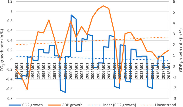
FIGURE 1. CO2 per capita and GDP growth rates in South Africa (1990–2018). Source: Authors’ illustration from World Bank Group, (2022).bib_world_bank_group_2023.
First, it is the first to analyze the effects of BCs on CO2 emissions in SA. The majority of studies on BCs in SA (Schumann, 1934; Du Plessis, 1951; Burger, 2011; Venter, 2019; Boshoff, 2020) focused on estimation and prediction. A close study on BC’s effects on environmental aspects involving SA is given by Li et al. (2022). Their study assessed the BC’s effects on energy intensity in BRICS and other emerging economies. Their findings suggest that during economic booms (recessions), BCs increase (lower) energy intensity. However, energy intensity is an intermediate victim of BCs. To provide a concrete environmental impact analysis of BCs, we extend the analysis to CO2 emissions in SA. Such an analysis is important to SA given its growth trajectory and growing regional and international economic relevance and vulnerability. SA is an emerging economy characterized by industrialization-induced increased growth. It is the biggest economy in Southern Africa, and has attracted increased ties with its regional peers characterized by weak and more vulnerable economies. Its vulnerability to BCs is also heightened by its growing connection with regional economic powerhouses outside Africa, particularly fellow BRICS countries. In the spirit of the Environmental Kuznets Curve (EKC) hypothesis, the BCs are likely to cause swings in CO2 emissions, making it difficult for SA to meet the net-zero emissions target. Accordingly, evidence from this study becomes important in answering whether, and how climate policy should respond to environmental degradation due to business fluctuations in SA. To the best of our knowledge, there exists no study that attempts to answer this research question in the context of sub-Saharan African countries and more importantly for SA. Thus, filling this gap is the first contribution of the present study.
Second, in this study, we shed light on whether or not, and how, CO2 emissions respond to business cycle shocks by deploying a battery of estimation techniques that consider the time-varying nature of the estimated marginal effects of CO2 emissions due to BCs. To recalibrate the methodological landscape by employing the rolling window regression and Markov-Switching-Dynamic-Regression (MSDR) approach to answer the specific question--whether the CO2 elasticities with respect to BCs in SA are time and regime-varying or not, respectively. The choice of extending the analytical purview to a developing economy (South Africa in this case), adds a novel dimension to the discourse. This strategic extension is not only a pragmatic choice but also an acknowledgment of the socio-economic specifics inherent in developing economies, introducing a distinctive narrative thread to the ongoing dialogue. In other words, this paper addresses the methodological voids in the existing literature by appreciating that emissions elasticity, rather than being a static parameter, is subject to change over time. Applying these techniques is important, given that it addresses the shortcoming of traditional time-series estimation methods, which tend to mask the time and regime-varying relationship between variables. For example, periods of statistically significant positive and negative impacts at different points in time could even out in the context of traditional econometric analysis, presenting evidence of no statistically significant effects. However, such evidence may not necessarily help in policy commendably as it is not likely to indicate how different events at different periods influenced the BCs-pollution nexus. The use of the rolling window regression framework and MSDR enables us to investigate the gradual process of environmental pollution transition and the role BCs have played in this process in SA.
The rest of this study is structured as follows. Section 2 provides the theoretical foundations and the related literature review of the growth-pollution nexus; Section 3 presents the overview of the data employed; Section 4 and 5 investigate (through the rolling window regression and MSDR approaches respectively) whether or not CO2 emissions elasticity is time-varying and if it differs during economic regimes. Section 6 presents and discusses the main results of the study and Section 7 concludes by providing key policy recommendations.
The relationship between economic growth and the environment is gaining a wide audience despite being a relatively new subject in economics. The most extensive theory is the Environmental Kuznets Curve (EKC) hypothesis developed from Kuznets (1955). It is theoretically rooted in classical economics. The EKC follows an inverted U-shape; environmental damage initially increases with growth in GDP and later decreases with increasing GDP. The inverted U-shaped curve represents pre-industrial (low-income economies) and beyond the turning point, post-industrial (high-income economies), where more resources will be availed for green technology investments (Abid, 2016). Transition from agricultural production into industrial production and its intensification result in increased pollution. With time, the industrial-heavy production will be phased out for more highly technological and service-centralized production that will counteract the pollution increase and eventually result in decreasing pollution levels per unit of output.
Contrary to the EKC theory, the World Commission on Environment and Development Report (WCED) of 1978 named “Our future” (commonly known as the Brundtland report, code named the Brundtland Curve Hypothesis (BCH)) presents another view of the relationship between GDP and environmental damage. It argued that poor countries initially cause high levels of environmental degradation, followed by a decrease in environmental degradation as economies grow until a turning point is reached, at which environmental degradation will then increase exhibiting a U-shaped BCH opposite to the inverted U-shaped EKC. As the economy grows, environmental damage decreases (poverty decreases). When the turning point is reached, pollution increases with GDP and eventually gets as high as originally. The positive trend in environmental degradation is caused by increased consumption, which leads to increased production. The environmental damage resulting from increased production is as damaging to the environment as the problems caused by poverty according to the theory (Etongo et al. (2016)).
The third theory is the Environmental Daly Curve hypothesis (EDCH) of 1973 by Daly. He described the relationship between economic growth and environmental damage by arguing that today’s economy driven by increased production is doomed and a steady-state type of economy could be the alternative. He further argued in 2004 that the impact of human creativity, innovation and green technology development is insufficient to lower pollution and offset the usage of scarce natural resources and the overall environmental damage. Incentives for a better, high-quality environment may occur when a country reaches a particular point of wealth, but environmental damage will already be too severe. Environmental damage increases with economic growth, no matter the willingness of the citizens and policymakers to counteract it (Daly and Farley, 2004). Therefore, the EDCH suggests that an increase in per capita GDP will lead to higher environmental damage (due to increased production). Hence, the EDCH does not depict a turning point at any level of wealth, such as the EKC and the Brundtland Curve (Bratt, 2012).
The nexus between business cycles and CO2 emissions is largely inspired by Jevons (1878a) hypothesis/theory, which provides an insight into how business cycles might influence CO2 emissions. Jevons took the view that changes in sunspots created comparable changes in crops, which in turn lead to business cycles. In his analysis of industrial depressions between 1721 and 1867, he discovered that a cycle of 10.43 years was almost indistinguishable when compared to that of sunspots. Based on this scientific observation he inferred that solar activity caused changes in weather, which in turn affected crops and the business cycle. Building on this hypothetical explanation, some standard economic theories have shed further light on the relationship between CO2 emission and business cycles. For example, the well-known classical theory underpinned by the assumption that the economy is self-regulating and functions best with negligible government intervention, does not allow for the possibility that business cycles might influence CO2 emissions. Contrarily, the Keynesian theory emerging in response to great depression proved that there is no self-regulating mechanism that guarantees full employment and that government intervention is needed to help economies deal with predicted or unpredicted business cycles. Recent theories such as the real business cycle have also emphasized the role of real factors (i.e., productivity or technology shock) as important drivers of macroeconomic fluctuations.
Premised on these theories/hypotheses, a growing body of empirical literature is paving the way for the link between business cycles and CO2 emissions, but with inconclusive findings (see Table 2). Doda (2014) utilized the HP filter method to examine the relationship between the cyclical components of emissions and GDP at business cycle frequencies of the period covering 1950–2011 in 122 countries. He found evidence to suggest that emissions are pro-cyclical (increasing during expansions and decreasing during recessions). Azami and Angazbani (2020) researched the association between CO2 emissions and business cycles for Asian and Middle Eastern countries that are known for being the largest emitters of carbon emissions (namely, China, India, Japan, Iran, Saudi Arabia, and South Korea) for the period 1960 to 2017. The findings of the Markov-switching autoregressive models also confirmed that emissions are more cyclical in most countries, with the exception of Iran. Similarly, Klarl (2020) examined the extent to which CO2 emissions are responsive to the business cycles for the United States during the period 1973 and 2015. Estimates derived from the rolling-regression approach and MSDR provide evidence in support of pro-cyclicity of CO2 emission. Reaching a similar conclusion, Heutel (2012) also established that carbon emissions were pro-cyclical for the U.S economy.
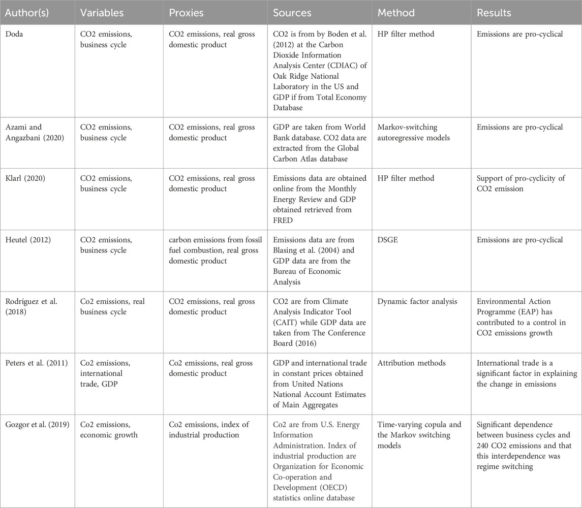
TABLE 2. Co2 emissions and business cycle: A brief review of literature.
A recent study by Sarwar (2021) conducted on South Asian countries found evidence to suggest that CO2 emissions are pro-cyclical and volatile. They also observed that the behavior of other emissions differs among countries. Technological shocks have varied effects, with improvements reducing CO2 emissions permanently in India and Bangladesh, and increasing them in Pakistan and Sri Lanka. Another recent study by Calvia (2022) investigated the cyclical interactions between the U.S. economy, fossil energy use, and air pollutants from 1990 to 2019. Findings reveal high volatility in both fossil energy use and air pollutants, with moderately high pro-cyclicality between fossil energy use (especially oil) and the business cycle. CO2 and CO exhibit similar pro-cyclicality, while other pollutants show weak associations with the business cycle.
The findings of pro-cyclicality of emissions are however not universal across studies. For example, while Alege et al. (2017) was probing the relationship between CO2 emissions and business cycles they concluded that large CO2 emissions are countercyclical to GDP, although somewhat pro-cyclical to agricultural output and the industrial sector of Nigeria. While investigating the link between the CO2 emissions and business cycles in the EU-28 for the period 1950 to 2012, using dynamic factor analysis, Rodríguez et al. (2018), found that the introduction of more stringent emissions targets since the fifth Environmental Action Programme (EAP) has contributed to a control in CO2 emissions growth in the EU. While examining the speed plus volatility of CO2 emissions relative to GDP, in developed and developing countries, Peters et al. (2011) found a speedy increase in CO2 emissions after economic recovery from Great Depression. Focusing on the interdependence between business cycles and CO2 emissions in the U.S economy, Gozgor et al. (2019) found that there exists a significant dependence between business cycles and CO2 emissions and that this interdependence was regime switching during the period 1973 to 2017.
Following a concise review of the existing literature, it becomes apparent that the analysis of the relationship between emissions and GDP at business cycle frequencies constitutes a relatively nascent area of research. The literature reveals a paucity of studies in this domain, with a notable concentration on the United States, leaving a significant gap in understanding the nuances of this relationship in a broader global context. Moreover, even the small number of existing literature reviewed here has generated more heat than light—remain inconclusive, confirming a narrative of a rather less obvious connection if any of economic activity and environmental effects. While a predominant inclination towards pro-cyclicality surfaces from the bulk of studies, the nuanced contradictions in the results accentuate the ins and outs intrinsic in this relationship. Indeed, a critical view taken by Klarl (2020) exposes an in-built assumption in the existing studies—an assumption of constant emissions elasticity over time. This assumption, constituting a methodological cornerstone, may overgeneralize the adaptive nature of the environmental response to changes in economic regimes. Klarl’s assertion that emissions elasticity is subject to temporal evolution during macroeconomic fluctuations aligns with broader trends observed in the data.
This objective of this paper is not merely to confirm or dispute prevailing conclusions but to recalibrate the methodological landscape by employing the rolling window regression and Markov-Switching-Dynamic-Regression (MSDR) approach to answer the specific question--whether the CO2 elasticities with respect to BCs in SA are time and regime-varying or not, respectively. The choice of extending the analytical purview to a developing economy (South Africa in this case), adds a novel dimension to the discourse. This strategic extension is not only a pragmatic choice but also an acknowledgment of the socio-economic specifics inherent in developing economies, introducing a distinctive narrative thread to the ongoing dialogue. In other words, this paper addresses the methodological voids in the existing literature by appreciating that emissions elasticity, rather than being a static parameter, is subject to change over time.
We use monthly data of Carbon dioxide (CO2) emissions (measured in metric tons per capita) collected from the World Bank Group, (2023)1. The nature of CO2 emissions data is from the manufacturing of cement and the burning of fossil fuels. It also includes emissions generated during consumption of liquid, solid, and gas flaring and gas fuels. For the business cycle, we employ monthly data of real GDP stem from the World Bank Group, (2023)2. Finally, for monetary policy shock, we use the South African Reserve Bank (SARB) repo rate and the data points are from the World Development Indicators of the World Bank Group, (2023)3. We decided to collect data starting from 1990 to 2018 for two reasons. First, the CO2 data for South Africa begins from 1990. Second, several macroeconomic research on business cycles in South Africa have occurred in the decade between 1990 and 2000, mostly with the turning point cycles identified by the SARB as an empirical starting point (Boshoff, 2020). Thus, our dataset spans a period from January 1990 to January 2018, which provides 337 observations.
Given that our interest is on the impact of business cycles, using raw data is not appropriate because it contains short-term movements associated with the business cycle (long-term trends). However, short-term fluctuations removal reveals long-term trends of time-series. Thus, we use the Hodrick-Prescott (HP) data filtering technique to eliminate the trend from our time-series. The HP filter is among the data-smoothing techniques that is commonly used in literature (Ravn and Uhlig, 2002), as it enables some low-frequency stochastic cycles to pass through. We illustrate the mechanics of this method by an example.
Assuming that the time series
where
We calculate the statistical properties of the variables of key interest (CO2 and GDP) using descriptive statistics, relative volatility, and cross-correlation coefficient. For example, Column 5 of Table 3 presents the outcome of the relative volatility of emissions, which is the ratio between the standard deviation of the cyclical component of CO2 emissions and the standard deviation of the cyclical component of GDP. Irrespective of which filtering technique is used, the outcome of the relative volatility is above 1, indicating that cyclical CO2 emissions are more volatile than GDP in post-Apartheid South Africa. This finding is consistent with Heutel (2012), Khan et al. (2015), and Klarl (2020) for the case of the United States. In column 6 of Table 3, we present the results of cross-correlation coefficient between the cyclical component of emissions and GDP. For all the data filtering techniques, the results indicate that CO2 emissions are positively correlated with GDP. Consequently, we partially conclude that CO2 emissions in South Africa are pro-cyclical by nature.5 In other words, this implies that CO2 emissions increase during expansions and decrease during recessions in South Africa. The next sections take this analysis further by using a more studious technical framework such as the Markov-Switching-Dynamic-Regression (MSDR).
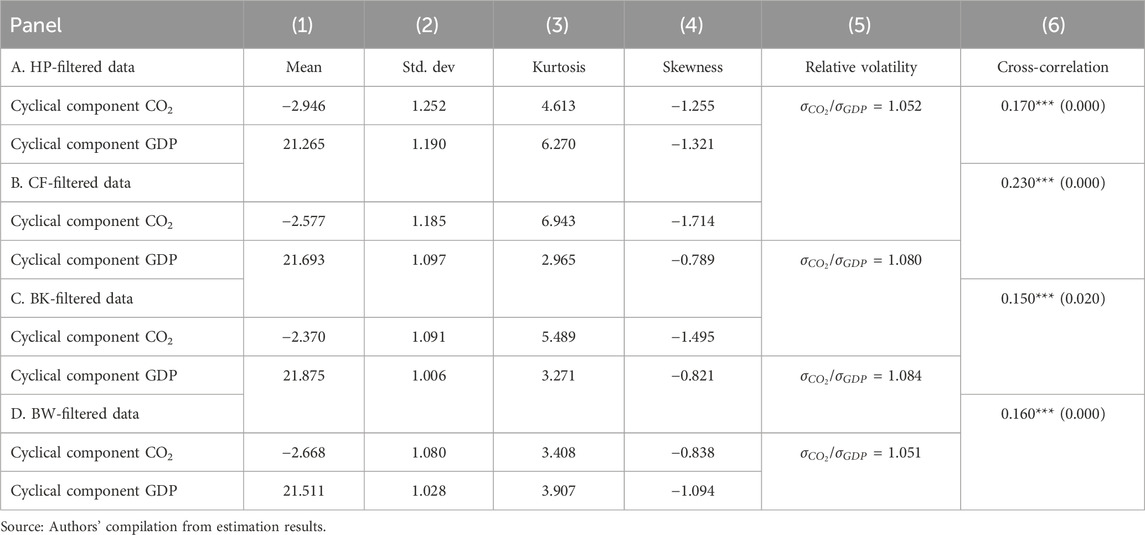
TABLE 3. Summary statistics.
As presented earlier, the objective of this study is to investigate the response of CO2 emissions to the business cycle for post-Apartheid South Africa. To achieve this, we follow a two-step strategy. First, we employ a rolling-window regression procedure to determine whether the CO2 emissions’ elasticity–with respect to changes in GDP–is time varying or not. Second, we use a MSDR framework to investigate the dynamics of the emissions to GDP relationship, across regimes. As shown in Eq. 2, for each of the four data filtering techniques employed, we run the following elementary regression:
where
The findings of the rolling-window regression are presented in Figure 2, with the estimated elasticity starting from 1991m1–2018m1. As reported in this figure, we show the estimated emissions’ elasticity for all the four filtering techniques. As can be seen in the figure, the green and blue line represents the estimated emissions’ elasticity with (
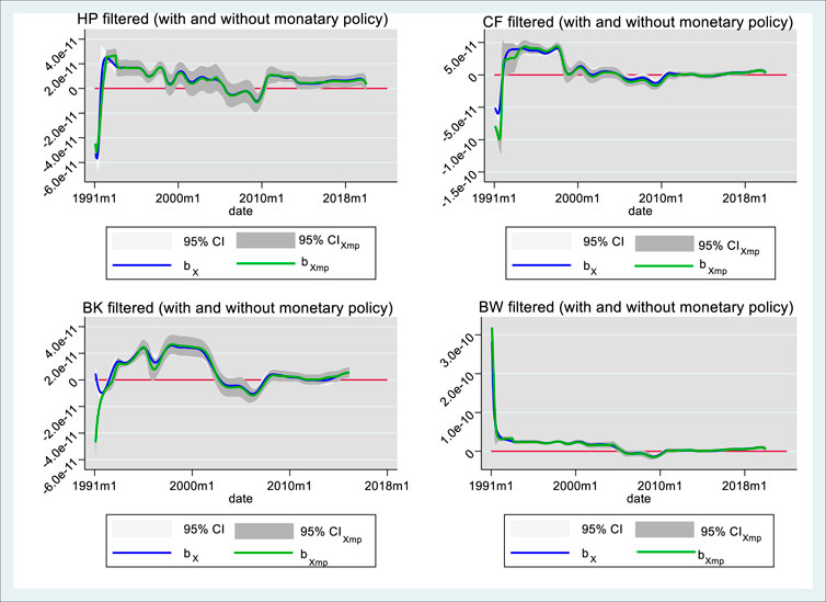
FIGURE 2. Rolling window regression coefficients of CO2 emissions for South Africa for different data filtering techniques. Source: Authors’ illustrations from rolling window estimation.
The blue and green lines are the time-varying CO2 emissions coefficients without and with the inclusion of monetary policy control respectively. The confidence intervals are 95%-bootstrapped with 5,000 replications. The shaded light and dark gray are confidence intervals without and with monetary policy control respectively. Notes:
The period of 1991–1993 is associated with the country’s third recession, while the 2008 to 2010 period is related to the recession caused by the recent financial crisis where South Africa’s growth has trended downwards since 2008. Among others, occasioning factors of the economic downturn included: declining commodity prices, the global downswing following the recent world financial crisis, deindustrialization, budgetary cuts, slowed investment as a result of economic stagnation, restrictive macroeconomic policies, ‘state capture’ (defined as a systemic institutional corruption), and insufficient electricity supply. Based on this finding, we observe that the emission’s elasticities are negative and statistically significant with respect to changes in GDP during recession periods and this is irrespective of which filtering technique is employed. This observation is key to justifying the use of MSDR framework to study the behaviour of emissions to business cycle, given that there is a clear impression that CO2 emissions respond differently in different economic regimes.
Additionally, the results in Supplementary Figure S1 of Supplementary Appendix SA1 are where we remove the repo interest rate (a variable used as a measure of monetary policy control) in the regression. The aim is to compare the real impact of the monetary policy shock in influencing emissions in South Africa. As seen in Figures 1, 4, our results indicate no significant difference when we include/remove the monetary policy control and this is irrespective of which data filtering method is employed. Lastly, Supplementary Figures S2, S3 of Supplementary Appendix SA2 present the results of the rolling-window regression with reduced and increased window size (window size is equal to 80 and 120 in Supplementary Figures S1, S2, respectively). The aim is to test the sensitivity of our estimation to changing the window size in the rolling-regression. As can be seen from both figures, the results remain qualitatively robust against decreasing/increasing the window size in the rolling-regression. This is a clear indication that the estimated emissions’ elasticity is time varying with economic boom and bust in South Africa. Our finding on the behaviour of CO2 emissions elasticity is similar to the finding of Klarl (2020) in the case of US economy. However, we consider this indication as a partial conclusion, which can be further explored with a more robust quantitative approach such as a regime-switching framework. Thus, we further study in the next section the emissions response to business cycle using MSDR framework.
The Markov-Switching-Dynamic-Regression (MSDR) is part of the Markov-switching frameworks used to model data that presents diverse dynamics across unobserved regimes/states through regime-dependent parameters (Mills and Wang, 2006; Guidolin, 2011a; 2011b). The MSDR is usually employed to accommodate multiple-regime phenomena such as structural breaks due to economic crises or policy reform (Garcia and Perron, 1996). The process of transitions between the unobserved regimes follows a process known in literature as “Markov chain”. Thus, the procedure enables for shifts in the intercept, explanatory variables (covariates), and variance (Klarl, 2020). In this study, we use the MSDR to ascertain whether the CO2 emissions’ elasticity with respect to changes in GDP is regime-dependent. Precisely, the MSDR technique enables us to answer the question whether CO2 emissions’ stock drops during recessions than in normal periods in South Africa. As indicated by Klarl (2020), an answer to this question is not only pertinent for optimal environmental policy formulation, but also calls the question of whether common solutions proposed through E-DSGE framework for optimal environmental policy are appropriate, viable or not.
Let us consider unobserved regimes/states that follow a Markov chain process (Quandt, 1972; Goldfeld and Quandt, 1973; Mills and Wang, 2006; Guidolin, 2011a; 2011b), the CO2 emissions evolution (details on the methodological framework of the Markov Switching Model are provided in Supplementary Appendix SA2 can be modeled as a regime-dependent intercept and covariate for regimes as shown in Eqs 3–6:
where
In the Markov Switching model, the probability distribution is expected to follow a logistic distribution (see Hamilton, 1994; Chen and Shen, 2007). The corresponding (N × N) matrix of transition probabilities is given by P =
We obtain unbiased point estimates in the MSDR by assuming the traditional assumption of zero covariance between the random walk and the state variable, cov (
According to economic theory, a business cycle goes through four distinguishable phases (expansion, peak, contraction or recession, and trough). On the one hand, the phase of expansion is the normal (GDP growth and is in the range of 2% and 3% per annum), while the peak is when the economic activity begins growing out of the 3% annual growth. On the other hand, contraction/recession is the abnormal phase when economic production is on the way down (GDP growth is below 2%), while the trough phase appears when recession phase reaches the bottom and begins to rebound into an expansion phase. A close look at the South African GDP growth rate data from 1990 to 2018 indicates two noticeable and dominant business cycle phases (recession and expansion). This leads us to define the business cycle of South Africa’s post-Apartheid period to two phases only
We perform five different MSDR models for each of the four data filtering method. In Model a, we consider an equal degree of volatility (
To decide which model is the best for prediction, forecast and policy, we use criteria such as model fit through information criteria and regime classification quality. Table 4 presents the results of the calculated values of different selection criteria for each of the five MSDR models and data filtering technique. From Table 4, we observe that the best model depends on the type of the data-filtering technique employed. In some cases, the information criteria are indecisive. As in Klarl (2020), we adopt models that are more general, especially, when we consider models that include monetary policy as a control variable. Hence, we work with Model (c1) for HP-filtered data, Model (a) for CF-filtered data, Model (c) for BK-filtered data, and Model (c1) for BW-filtered data. Finally, we check the significance (regime-dependent role) of the monetary policy control by the means of Wald-test and Student’s t-test.
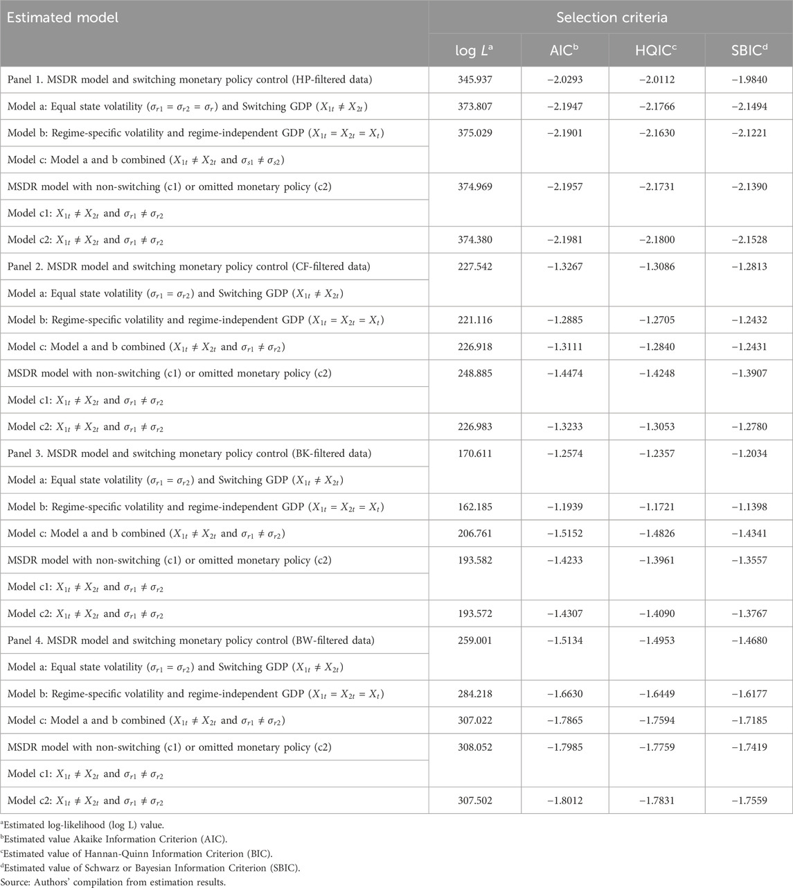
TABLE 4. Two-regime MSDR model fit.
Table 5 shows the results of the estimated MSDR for each selected model. Panel A of Table 5 displays the results of the estimated CO2 emissions’ elasticity due to changes in GDP. Panel B of Table 5 reports the results of the regime-specific volatility estimates, while Panel C of Table 5 shows the probabilities of transition from regime 1 to regime 2. Finally, Panel D of Table 5 reports the duration it takes for emissions to shift from regime 1 to regime 2.

TABLE 5. Results for selected MSDR models.
By focusing on the results in Panel A of Table 5, we observe clear evidence of CO2 emissions smoothing from regime 1 to regime 2 in South Africa, irrespective of which data-filtering technique is considered. For example, the results of Model c1 as selected for HP-filtered data assumes regime-switching behavior of GDP. Specifically, the results indicate a significantly negative CO2 emissions’ elasticity with a value of −0.000264 (regime 1) and a significantly positive CO2 emissions elasticity with a value of 0.000192 (regime 2). These estimated elasticities imply that regime 1 is categorized as the low CO2 emissions regime while regime 2 is categorized as the high CO2 emissions regime. Although our results differ with those of Klarl (2020) in terms of the sign and magnitude of the estimated CO2 emissions elasticities, however, they confirm his findings in relation to the presence of low and high CO2 emissions regime in South Africa in the post-Apartheid period. Moreover, our estimated elasticities are in line with Heutel’s (2012) findings for the U.S economy.
We have also obtained some insightful information from the probabilities of transition and duration of persistence of CO2 emissions. We obtain an estimate of 0.951 (95.1%) probability indicating that a low CO2 emissions regime in the current month will stay low in the next month but a 5% chance that it will transit to a high CO2 emissions regime in the following month. On the other hand, our estimation shows that there is a 3.88% chance that low CO2 emissions in the current month would transit to high CO2 emissions in the next month. Besides, there is a 96.12% chance that a low CO2 emissions regime in the current month would stay low in the following month. In other words, this finding clearly indicates that both regimes are highly persistent. Concerning the duration of transition, the results indicate that the first regime (regime 1) takes approximately 20 months (six and half quarter); while the second regime (regime 2) transits into the next regime in approximately 25 months (8 quarters); since Model c1 included the reserve bank repo rate as an additional policy shock besides productivity shock.
It is worth noting that both transitions and persistence of emissions in this model are with the consideration of monetary policy control. Finally, our statistical testing shows evidence for a regime-specific volatility, where the Wald test statistics rejects the null hypothesis of equal error term variances (see Panel C). For the CF filtering technique, the results are similar to those of the HP filtering method: The Model (a) result also suggests regime-switching behavior of GDP. Specifically, we found a significantly negative CO2 emissions’ elasticity with a value of −0.000119 (regime 1) and a significantly positive CO2 emissions’ elasticity with a value of 0.00040 (regime 2). We found a transitional duration of 44 months (14 quarters) in regime 1 and 24 months (8 quarters) in regime 2. In addition, the transitional probabilities (0.97 in regime 1 and 0.041 in regime 2) indicate that both regimes are highly persistent.
Contrary to the HP and CF filtered data, the BK filtered data suggests a regime-switching behavior of GDP but the CO2 emissions elasticity for regime 1 is not statistically significant, although it has the expected negative sign. Moreover, the Wald test statistics rejects the null hypothesis of equal emissions’ elasticity as well as equal regime volatility at the 1% significance level. The transitional duration in both regimes is nearly the same with 18 months (6 quarters) on average. The results for the BW data filtering technique also points out to regime-switching behavior of GDP. Henceforth, the results are the same as the ones we obtain for the HP data filtering method. Furthermore, in Figure 3, we provide an economic interpretation of the obtained regimes. First, as in Klarl (2020), we used the smoothed transition probabilities and regime classifications (low and high regime) to reproduce South Africa’s cyclicality of emissions. Second, we follow the Chevallier and Goutte (2017) and Klarl (2020) procedure and plug the identified regimes back to the transition probabilities data.
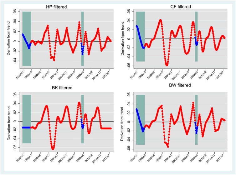
FIGURE 3. Regime-dependent cyclicality of CO2 emissions in South Africa post-Apartheid periods. Source: Authors’ illustration from regression results.
Blue small circles are associated with an economic downturn (low regime
As can be seen from Figure 3, the blue small circles are associated with an economic downturn (low regime
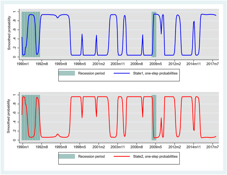
FIGURE 4. Markov-switching dynamic regression smoothed regime probabilities for HP-filtered data method. Source: Authors’ illustration from regression results.
Because of the growing challenges of global warming and climate change, researchers have become more interested in the determinants of these issues. According to empirical studies, climate change is mostly linked to environmental degradation (as measured by CO2 emissions) (see Lopez-Menendez et al., 2014). Given the foregoing, recent empirical studies have typically focused on the relationship between economic growth and environmental quality (CO2 emissions), as economic expansion has been identified as a major driver of environmental degradation. However, empirical evidence from emerging market economies is quite scarce. This paper is thus related to the incipient literature on the relationship between CO2 emissions and business cycles (measured by GDP fluctuations) in South Africa.
Specifically, the study peruse two distinct objectives. First, we analyze the effects of business cycles on CO2 emissions in South Africa. Second, we shed light on whether or not, and how, CO2 emissions respond to business cycle shocks by deploying a battery of estimation techniques that consider the time-varying nature of the estimated marginal effects of CO2 emissions due to business cycles. The study focuses on South Africa because it is an emerging economy characterized by industrialization-induced increased growth. Also, it is the second biggest economy in sub–Saharan Africa (SSA), and has attracted increased ties with its regional peers characterized by weak and more vulnerable economies. South Africa’s vulnerability to business cycle fluctuations is also heightened by its growing connection with regional economic powerhouses outside Africa, particularly fellow BRICS countries. In light of this, the study performs three critical analyses. First, given that our interest is on the impact of business cycle on CO2 emissions, we use the Hodrick-Prescott (HP) data filtering technique to eliminate the trend from our time-series data. The HP filter technique, which is a data-smoothing procedure enables some low-frequency stochastic cycles to pass through. From the data filtering technique, we show that CO2 emissions are positively correlated with GDP. Accordingly, we partly conclude that CO2 emissions in South Africa are procyclical by nature.
In the next part, we use a rolling-window procedure to determine whether the CO2 emissions’ elasticity, with respect to changes in GDP, is time varying or not. We set the window size to 35% of the total number of observations to allow sufficient smoothing and minimization of white noise in the parameters, while at the same time allowing for an examination of the variability in the coefficients. Results from the rolling-window shows that the estimated emissions’ elasticity and the corresponding confidence interval are unstable throughout the study period. Moreover, the estimated emissions’ elasticity is significant at the 5% level of significance. This result reinforces our findings in the filtering technique. Hence, we conclude that from the years 1993–2007, the estimated emissions’ elasticity has a more pronounced positive behavior. In addition, the result from the rolling-window indicates that for a relatively short period going from the years 1991–1992 and 2008 to 2010, the estimated emissions’ elasticity has a more pronounced negative behaviour. We conclude that this downturn might have been primarily occasioned by the fact that the country experienced a recession between 1991–1993 and the global financial crisis in 2008. Additionally, we remove the repo interest rate, which is a measure of monetary policy to compare the real impact of the monetary policy shock in influencing emissions in South Africa. Our results show no significant difference when we include or remove the monetary policy control and this is irrespective of which data filtering method is employed. Moreover, we also undertake analysis of decreased and increased rolling-window–window size equal to 80 and 120 to test the sensitivity of our estimation to changes in the window size. Our results remain qualitatively robust against decreasing/increasing the window size in the rolling-regression. We conclude that the estimated emissions’ elasticity is time varying with economic boom and bust in South Africa.
The third unique feature of our study is that, we use a Markov-Switching-Dynamic-Regression (MSDR) to further investigate CO2 emissions response to business cycles. The MSDR has the strength to accommodate multiple-regime phenomena such as structural breaks owing to factors such as economic crises or policy reform. Findings from the MSDR show evidence of CO2 emissions smoothing from regime 1 to regime 2 in South Africa. Specifically, the results indicate a significantly negative CO2 emissions’ elasticity in regime 1 and, a significantly positive CO2 emissions’ elasticity in regime 2. We conclude that, the estimated elasticities suggest that regime 1 is categorized by low CO2 emissions while regime 2 is categorized by high CO2 emissions. Also, the MSDR results shows that there is lower probability that low CO2 emissions in the current month would transit to high CO2 emissions in the next month. In addition, there is a higher a probability that a low CO2 emissions regime in the current month would stay low in the following month. Regarding the temporal aspect of the transition process, our findings reveal valuable insights into the duration of each regime. The analysis indicates that the initial regime, denoted as regime 1, spans a duration of approximately 20 months, equivalent to six and a half quarters. This signifies a notable period during which the economic dynamics and policy shocks associated with regime 1 are influential and persistent. In contrast, the transition to the subsequent regime, denoted as regime 2, unfolds over a span of approximately 25 months, equivalent to 8 quarters. It is noteworthy that in Model c1, the inclusion of the reserve bank repo rate as an additional policy shock, alongside the productivity shock, contributes to the dynamics observed in regime 2. This extended duration suggests a more prolonged and intricate shift in economic conditions, policy responses, and other relevant factors that characterize the second regime. The detailed breakdown of these transition durations provides a nuanced understanding of the temporal evolution between regimes. The 20-month duration for regime 1 implies a substantial period of stability or distinctive economic conditions that define the initial phase. On the other hand, the 25-month transition to regime 2 suggests a more gradual and complex adjustment, potentially influenced by the interplay of multiple policy shocks and economic variables.
Our findings have several policy implications. Firstly, policymakers can implement certain policy changes to reduce CO2 emissions in South Africa. As demonstrated by our results, achieving increased growth would put pressure on CO2 emissions, necessitating strong and equitable energy transitioning. Therefore, in order to reduce greenhouse gas (GHG) emissions, policymakers should consider the business cycle phase when implementing environmental policies. The consequences of neglecting the asymmetric influence of the business cycle on emissions are significant. Emission forecasts that disregard this dynamic element may present an incomplete and potentially misleading picture. This incomplete understanding could lead to the development of policies that are not finely matched to the prevailing economic conditions. In response to this, we assert that policymakers need to be cognizant of the business cycle’s impact on emissions to ensure that policy initiatives are appropriately tailored to the local economic dynamics. For example, as South Africa endeavors to meet its 2030 energy sustainability objective of reducing greenhouse gas emissions, policymakers can leverage environmental policies to achieve the stipulated targets. Strategies such as promoting energy efficiency and implementing carbon levies emerge as effective tools in attaining the 2030 goals for greenhouse gas emission reductions. Specifically, we advocate for the design of carbon-pricing policies in a countercyclical fashion. This implies that emissions should be priced disproportionately towards the business cycle upswing, aligning with periods of economic growth.
Secondly, our findings show that CO2 emissions respond to changes in economic growth. We therefore recommend a steadfast commitment to the reinforcement of research efforts in the domains of energy management, production, and energy-saving technology. This strategy can reduce CO2 emissions significantly without impeding South Africa’s present development trajectory. In particular, we advocate for an unwavering dedication by South African policymakers to allocate resources and prioritize budgetary tools that support research and development (R&D) in industrial technologies geared towards energy conservation. The literature underscores the potential of investing in renewable energy sources as a linchpin for mitigating CO2 emissions. Hence, fostering innovation in energy-related sectors is pivotal for achieving sustained reductions in CO2 emissions. This commitment not only bolsters the nation’s technological capabilities but also positions it at the forefront of global efforts to transition towards cleaner, more sustainable energy practices. Moreover, the emphasis on resource allocation and budget underscores the need for strategic financial investments to catalyze the development and implementation of energy-saving technologies. South African policymakers should view these investments as integral components of a forward-looking strategy, recognizing that the benefits extend beyond immediate gains in emissions reduction. The long-term impacts involve skills acquisition and job creation for the youth of South Africa.
Thirdly, our results show regime-switching behavior of GDP, indicating significantly negative CO2 emissions during recessions and positive emissions during expansions. In light of this, we recommend the importance of tailoring strategies to various stages of South Africa’s economy, with a specific focus on crafting specialized initiatives to reduce greenhouse gas (GHG) emissions, particularly within the industrial sector. This nuanced approach recognizes the diverse economic landscape and the varying challenges posed by different sectors of the South African economy. We strongly emphasize the need for targeted policies that address the unique characteristics of each stage of economic growth in South Africa. For example, the industrial sector, identified as a significant contributor to CO2 emissions in South Africa, requires specific attention. Emissions stemming from activities such as the burning of fossil fuels and cement production have been pinpointed as major drivers of CO2 (see Roser and Rosado, 2020). Therefore, policymakers should design and implement measures that not only curtail the consumption of fossil energy but also strategically optimize and enhance the use of clean alternative energy sources. This involves promoting and incentivizing the adoption of sustainable practices and technologies within the industrial sector.
Lastly, our findings demonstrates that initiatives designed to spur economic growth should not come at the expense of environmental deterioration. We advocate for the use of fiscal policies in mitigating CO2 emissions most importantly in developing economies. This could take the form of maintaining an ideal level of government spending and taxation, especially during cyclical downturns in the economy. To achieve this, policymakers can set emission intensity targets and implement emission caps, thereby establishing benchmarks to regulate and reduce carbon emissions across industries. Emission intensity targets could serve as a metric to gauge the level of emissions produced per unit of economic activity in South Africa. By setting and enforcing these targets, policymakers can ensure that industries are held accountable for their environmental impact. Simultaneously, implementing emission caps places an upper limit on the total amount of emissions allowed within a specified period, providing a tangible framework for reducing overall carbon output in South Africa and across the globe.
Even though our findings are robust across all the data filtering techniques, however, there is a caveat to our study. Our findings suggest that CO2 emissions are procyclical in South Africa; however, the behaviour of CO2 emissions changes from country to country. Therefore, a one-size-fits-all policy designed to mitigate CO2 emissions and boost growth may not yield the same outcome in other parts of the world. We propose that future studies undertake further analysis using a cross country dataset to show the heterogeneity among countries. Furthermore, we also recommend a more empirical exploration through the prism of a structural model that weighs the advantages and disadvantages of taxes on emissions. This could shed more light on the efficacy of using fiscal policies to mitigate CO2 emissions.
The raw data supporting the conclusion of this article will be made available by the authors, without undue reservation.
DE: Conceptualization, Data curation, Formal Analysis, Methodology, Writing–original draft. RS: Conceptualization, Data curation, Formal Analysis, Investigation, Writing–original draft, Writing–review and editing. BM: Investigation, Validation, Writing–original draft, Writing–review and editing. FB: Data curation, Formal Analysis, Methodology, Software, Validation, Writing–original draft, Writing–review and editing. SM: Validation, Writing–original draft, Writing–review and editing.
The author(s) declare financial support was received for the research, authorship, and/or publication of this article. RS was supported through a South African Department of Science and Innovation and National Research Foundation (DSI-NRF) Risk and Vulnerability Science Centre award to the Afromontane Research Unit (ARU) (University of the Free State; Grant No. 128386).
The authors declare that the research was conducted in the absence of any commercial or financial relationships that could be construed as a potential conflict of interest.
All claims expressed in this article are solely those of the authors and do not necessarily represent those of their affiliated organizations, or those of the publisher, the editors and the reviewers. Any product that may be evaluated in this article, or claim that may be made by its manufacturer, is not guaranteed or endorsed by the publisher.
The Supplementary Material for this article can be found online at: https://www.frontiersin.org/articles/10.3389/fenvs.2023.1321335/full#supplementary-material
1https://data.worldbank.org/indicator/EN.ATM.CO2E.PC.
2https://data.worldbank.org/indicator/NY.GDP.MKTP.CD.
3https://data.worldbank.org/indicator/FR.INR.RINR.
4For details see Hodrick and Prescott (1997), Christiano and Fitzgerald (2003), Baxter and King (1999), and Butterworth (1930).
5It is obvious that several market rigidities and frictions such as wage rigidities or simply labour adjustment costs also affect a country’s business cycle. Therefore, monetary policy control is not the only variable that can explain the emissions’ behaviour across the frequency of the business cycle. An inclusion in the model of other relevant controls might shed more light as to which shocks are most important for explaining the emissions’ behaviour during the business cycle frequency.
6Each regression we run using 95% bootstrapped confidence interval employ a total number of 5,000 replications.
7Heutel (2012) employs both monthly and quarterly data, while Klarl (2020) employs quarterly data to study the response of emissions to changes in economic activity in the case of United States. They both found results that are similar to this current study.
8See Hamilton (Hamilton, 1994, chapter 22) and Krolzig (1997, Chapter5) who provide more technical details on how to construct likelihood function with latent states.
9We have only presented the smoothed regime probabilities figure for the HP filtered data. The figures for the rest of data filtering methods can be made available upon request.
Alege, P. O., Oye, Q.-E., Adu, O. O., Amu, B., and Owolabi, T. (2017). Carbon emissions and the business cycle in Nigeria. Int. J. Energy Econ. Pol. 7 (5), 9. Available at: https://www.econjournals.com/index.php/ijeep/article/view/5076/3274.
An, Z., Jalles, J. T., and Loungani, P. (2018). How well do economists forecast recessions? IMF Work. Pap. 21 (2), 100–121. WP/18/39. doi:10.1111/infi.12130
Annicchiarico, B., Carattini, S., Fischer, C., and Heutel, G. (2021). Business cycles and environmental policy: a primer. Environ. Energy Policy Econ. 3, 221–253. doi:10.1086/717222
Arora, V. (2005). “Economic growth in post-apartheid,” in Post-apartheid South Africa: the first ten years. Editors M. Nowak, and L. A. Ricci (Washington, D.C., USA: International Monetary Fund), 13–22.
Azami, S., and Angazbani, F. (2020). CO2 response to business cycles: new evidence of the largest CO2-Emitting countries in Asia and the Middle East. J. Clean. Prod. 252, 119743. doi:10.1016/j.jclepro.2019.119743
Boshoff, W. H. (2020). Business cycles and structural change in South Africa. http://link.springer.com/10.1007/978-3-030-35754-2.
Bratt, L. (2012). “Three totally different environmental/GDP curves,” in Sustainable DevelopmentEducation, business and management-architecture and building construction-agriculture and food security (London, UK: Intechopen).
Burger, P. (2011). The South African business cycle: what has changed? South Afr. J. Econ. Manag. Sci. 13 (1), 26–49. doi:10.4102/sajems.v13i1.197
Calderón, C., and Fuentes, R. (2010). Characterizing the business cycles of emerging economies. https://papers.ssrn.com/sol3/papers.cfm?abstract_id=1629052.
Calvia, M. (2022). Business cycles, fossil energy and air pollutants. United States: U.S. “stylized facts”.
Chen, S.-W., and Shen, C. H. (2007). A sneeze in the U.S., a cough in Japan, but pneumonia in Taiwan? An application of the Markov-switching vector autoregressive model. Econ. Model. 24, 1–14. doi:10.1016/j.econmod.2006.04.012
Chevallier, J., and Goutte, S. (2017). On the estimation of regime-switching Lévy models. Stud. Nonlinear Dyn. Econ. 21, 3–29. doi:10.1515/snde-2016-0048
Daly, H., and Farley, J. (2004). Introduction to ecological economics. Washington, DC: Island Press.
Doda, B. (2014). Evidence on business cycles and emissions. J. Macroecon. 40, 214–227. doi:10.1016/j.jmacro.2014.01.003
Dominioni, G., and Faure, M. (2022). Environmental policy in good and bad times: the countercyclical effects of carbon taxes and cap-and-trade. J. Environ. Law 35 (05), 269–286. doi:10.1093/jel/eqac003
Du Plessis, J. C. (1951). Economic fluctuations in South Africa: 1910-1949 (No. 2). Bureau for economic research, faculty of commerce of the university of stellenbosch. Cambridge, England: Cambridge University Press.
Edwards, M. R., Klemun, M., Kim, H. C., Wallington, T. J., Winkler, S. L., Tamor, M. A., et al. (2017). Vehicle emissions of short-lived and long-lived climate forcers: trends and tradeoffs. Faraday Discuss. 200, 453–474. doi:10.1039/c7fd00063d
Espoir, D. K., and Ngepah, N. (2021). Income distribution and total factor productivity: a cross-country panel cointegration analysis. Int. Econ. Econ. Policy 8 (4), 661–698. doi:10.1007/s10368-021-00494-6
Espoir, D. K., and Sunge, R. (2021). Co2 emissions and economic development in Africa: evidence from a dynamic spatial panel model. J. Environ. Manag. 300, 113617. doi:10.1016/j.jenvman.2021.113617
Field, B. C., and Field, M. K. (2013). Environmental economics - an introduction. New York: McGraw-Hill Education.
Garcia, R., and Perron, P. (1996). An analysis of the real interest rate under regime shifts. Rev. Econ. Statistics 78, 111–125. doi:10.2307/2109851
Geels, F. W. (2013). Sustainability transitions: financial investment, the impact of the financial-economic crisis on governance and public discourse. https://www.econstor.eu/handle/10419/125691.
Goldfeld, S. M., and Quandt, R. E. (1973). A Markov model for switching regressions. J. Econ. 1, 3–15. doi:10.1016/0304-4076(73)90002-x
Gozgor, G., Tiwari, A. K., Khraief, N., and Shahbaz, M. (2019). Dependence structure between business cycles and CO2 emissions in the US: evidence from the time-varying Markov-Switching Copula models. Energy 188, 115995. doi:10.1016/jenergy2019115995
Guidolin, M. (2011a). “Markov-switching in portfolio choice and asset pricing models: a survey,” in Missing data methods: time series methods and applications. Editor D. M. Drukker (Bingley, UK: Emerald).
Guidolin, M. (2011b). “Markov-switching models in empirical finance,” in Missing data methods: time series methods and applications. Editor D. M. Drukker (Bingley, UK: Emerald).
Hall, B. V., and Thomson, P. (2021). Does Hamilton’s OLS regression provide a “better alternative” to the hodrick-prescott filter? A New Zealand business cycle perspective. J. Bus. Cycle Res. 17, 151–183. doi:10.1007/s41549-021-00059-1
Hamilton, J. D. (1994). Time series analysis. Princeton New Jersey. J. Econ. 60, 1–22. Available at: https://press.princeton.edu/books/hardcover/9780691042893/time-series-analysis.
Heutel, G. (2012). How should environmental policy respond to business cycles? Optimal policy under persistent productivity shocks. Rev. Econ. Dynam 15 (2), 244–264. doi:10.1016/j.red.2011.05.002
Jevons, W. S. (1878a). The periodicity of commercial crises, and its physical explanation. J. Stat. Soc. Inq. Soc. Irel., 334–342. Available at: http://www.tara.tcd.ie/handle/2262/8261.
Khan, H., Knittel, C. R., Metaxoglou, K., and Papineau, M. (2015). “How do carbon emissions respond to business-cycle shocks?,” in MIT CEEPR working paper (Cambridge, MA, USA: MIT CEEPR), 15–05.
Kim, C. J. (1994). Dynamic linear models with Markov switching. J. Econ. 64, 1–22. doi:10.1016/0304-4076(94)90036-1
Klarl, T. (2020). The response of CO2 emissions to the business cycle: new evidence for the US. Energy Econ. 85, 104560. doi:10.1016/j.eneco.2019.104560
Klein, P. A., and Moore, G. H. (1985). Monitoring growth cycles in market-oriented countries: developing and using international economic indicators. Philadelphia, Pennsylvania, United States: Ballinger.
Kuznets, S. (1955). Economic growth and income inequality. Am. Econ. Rev. 45 (1), 1–28. Available at: https://www.jstor.org/stable/1811581.
Li, T., Li, X., and Liao, G. (2022). Business cycles and energy intensity. Evidence from emerging economies. Borsa Istanb. Rev. 22 (3), 560–570. doi:10.1016/j.bir.2021.07.005
Marumoagae, M. C. (2014). The effect of the global economic recession on the South African labour market. Mediterr. J. Soc. Sci. 5 (23), 380–389. doi:10.5901/mjss.2014.v5n23p380
Mills, T., and Wang, P. (2006). Modelling regime shift behaviour in Asian real interest rates. Econ. Model. 23 (6), 952–966. doi:10.1016/j.econmod.2006.04.007
Nemet, G. F., Grubler, A., and Kammen, D. M. (2016). Countercyclical energy and climate policy for the U.S. Wiley Interdiscip. Rev. Clim. Change 7 (1), 5–12. doi:10.1002/wcc.369
Peters, G. P., Minx, J. C., Weber, C. L., and Edenhofer, O. (2011). Growth in emission transfers via international trade from 1990 to 2008. Proc. Natl. Acad. Sci. U. S. A. 108, 8903–8908. doi:10.1073/pnas.1006388108
Quandt, R. E. (1972). A new approach to estimating switching regressions. J. Am. Stat. Assoc. 67, 306–310. doi:10.1080/01621459.1972.10482378
Ravn, M. J., and Uhlig, H. (2002). On adjusting the Hodrick-Prescott filter for the frequency of observations. Rev. Econ. Stat. 84 (2), 371–376. doi:10.1162/003465302317411604
Rena, R., and Msoni, M. (2017). Global financial crises and its impact on the South African economy: a further update. J. Econ. 5 (1), 17–25. doi:10.1080/09765239.2014.11884980
Rodríguez, M. J. D., Ares, A. C., and de Lucas Santos, S. (2018). Cyclical fluctuation patterns and decoupling: towards common EU-28 environmental performance. J. Clean. Prod. 175, 696e706. doi:10.1016/j.jclepro.2017.11.244
Roser, M., and Rosado, P. (2020). CO- and greenhouse gas emissions. https://ourworldindata.org/co2-emissions?utm_source=tri-city%20news&utm_campaign=tricity%20news%3A%20outbound&utm_medium=referra.
Sarwar, , Ali, S., and Hussain, H. (2021). Business cycle fluctuations and emissions: evidence from South asia. J. Clean. Prod. 298, 126774. doi:10.1016/j.jclepro.2021.126774
Schumann, C. G. W. (1934). Business cycles in South Africa, 1910–1933: an analysis of some statistical series and of certain aspects of the business cycle and business forecasting. South Afr. J. Econ. 2 (2), 130–159. doi:10.1111/j.1813-6982.1934.tb01890.x
Venter, J., and Pretorius, W. (2001). A note on the business cycle in South Africa during the period 1997 to 1999.
Venter, J. C. (2019). “A brief history of business cycle measurement in South Africa,” in Business cycles in BRICS. Editors S. Smirnov, A. Ozyildirim, and P. Picchetti (Berlin, Germany: Springer), 185–211.
Woodford, M. (2003). Interest and prices – foundations of a theory of monetary policy. Princeton, New Jersey, United States: Princeton University Press.
World Bank Group (2023). World development Indicators (WDI) online. http://data.worldbank.org/data-catalog/world-development-indicators.
Keywords: business cycle, CO2 emissions, rolling window regression, markov-switching, South Africa
Citation: Espoir DK, Sunge R, Mduduzi B, Bannor F and Matsvai S (2024) Analysing the response of CO2 emissions to business cycle in a developing economy: evidence for South Africa post-apartheid era. Front. Environ. Sci. 11:1321335. doi: 10.3389/fenvs.2023.1321335
Received: 13 October 2023; Accepted: 05 December 2023;
Published: 19 January 2024.
Edited by:
Faik Bilgili, Erciyes University, TürkiyeCopyright © 2024 Espoir, Sunge, Mduduzi, Bannor and Matsvai. This is an open-access article distributed under the terms of the Creative Commons Attribution License (CC BY). The use, distribution or reproduction in other forums is permitted, provided the original author(s) and the copyright owner(s) are credited and that the original publication in this journal is cited, in accordance with accepted academic practice. No use, distribution or reproduction is permitted which does not comply with these terms.
*Correspondence: Regret Sunge, c3VuZ2VyMUB1ZnMuYWMuemE=
Disclaimer: All claims expressed in this article are solely those of the authors and do not necessarily represent those of their affiliated organizations, or those of the publisher, the editors and the reviewers. Any product that may be evaluated in this article or claim that may be made by its manufacturer is not guaranteed or endorsed by the publisher.
Research integrity at Frontiers
Learn more about the work of our research integrity team to safeguard the quality of each article we publish.