 Elton L. Cao
- Fairview High School, Boulder, CO, United States
Outdoor air pollution, specifically nitrogen dioxide (NO2), poses a global health risk. Land use regression (LUR) models are widely used to estimate ground-level NO2 concentrations by describing the satellite land use characteristics of a given location using buffer distance averages of variables. However, information may be leaked in this approach as averages ignore the variances within the averaged region. Therefore, in this study, we leverage a convolutional neural network (CNN) architecture to directly pass data grids of various satellite data for the prediction of U.S. national ground-level NO2. We designed CNN architectures of various complexity which inputs both satellite and meteorological reanalysis data, testing both high and low resolution data grids. Our resulting model accurately predicted NO2 concentrations at both daily (R2 = 0.892, RMSE = 2.259, MAE = 1.534) and annual (R2 = 0.952, RMSE = 0.988, MAE = 0.690) temporal scales, with coarse resolution imagery and simple CNN architectures displaying the best and most efficient performance. Furthermore, the CNN outperforms traditional buffer distance models, including random forest (RF), feedforward neural network (FNN), and multivariate linear regression (MLR) approaches, resulting in the MLR performing the poorest at daily (R2 = 0.625, RMSE = 4.281, MAE = 3.102) and annual (R2 = 0.758, RMSE = 2.218, MAE = 1.652) scales. With the success of the CNN in this approach, satellite land use variables continue to be useful for the prediction of NO2. Using this computationally inexpensive model, we encourage the globalization of advanced LUR models as a low-cost alternative to traditional NO2 monitoring.
Introduction
Outdoor air pollution was identified as the largest environmental cause of attributable deaths, associated with several negative health effects including respiratory illnesses and cerebrovascular diseases (Lelieveld et al., 2015; GBD, 2016). Specifically, nitrogen dioxide (NO2), a prevalent pollutant emitted through the burning of fuel, is linked to asthma and increased cardiac and respiratory mortality (Chiusolo et al., 2011; Greenberg et al., 2016). With the prevalence of NO2 in urban settings and a substantial portion of the world’s population living in cities, models which can estimate ground-level NO2 concentrations are crucial to appropriately assess human exposure and enact policy changes to ultimately provide a better air environment to inhabit (Novotny et al., 2011; Costa et al., 2014). In the United States, environmental disparities of NO2 concentrations between majority and minority groups are increasingly evident, indicating a demand for environmental justice (Clark et al., 2014).
Physical models that simulate chemical and physical processes involved with emission formation have long been used to quantify ground-level NO2 concentrations, including the Community Multiscale Air Quality (CMAQ) and the Global Environmental Multiscale (GEM) models (Byun and Schere, 2006; Kaminski et al., 2008). However, despite these models’ adaptability and interpretability of pollutant processes, they are computationally expensive and require a complete assessment of pollution sources and processes (Zhang et al., 2012). Statistical models, including various multivariate models, have emerged as a more cost effective alternative, albeit with a decrease in performance (Zhang et al., 2012; Finazzi et al., 2013). One of the most common statistical models is the land use regression (LUR) model, which aims to fit a multivariate model based on various land use characteristics to estimate monitored concentrations (Hoek et al., 2008; Knibbs et al., 2014; Larkin et al., 2017). LUR models have been developed for both national and global scales (Larkin et al., 2023), as well as for various countries including the United States (Novotny et al., 2011), Australia (Knibbs et al., 2014), Canada (Liu et al., 2020), and sections of Europe (De Hoogh et al., 2013). These LUR models rely on information from satellite data in the form of buffer distances (Hoek et al., 2008).
Machine learning (ML) has shown promise in enhancing predictive capacity of statistical LUR models (Kang et al., 2018). Various ML models, including random forests (RF) (Zhan et al., 2018), artificial neural networks (ANN) (Chan et al., 2021), and support vector machines (SVM) (Sánchez et al., 2011), have outperformed linear statistical models by providing necessary nonlinearity to satellite imagery (Kang et al., 2018). Gharamanloo et al. (2021) developed a 1D Deep-CNN model which was found to outperform linear statistical models in estimating NO2 concentrations in Texas. Kang et al. (2021) implemented a variety of ML approaches, including RF, SVM, and Extreme Gradient Boost (XGB) models, to infer NO2 concentrations in East Asia and significantly improved on linear regression approaches.
However, with these models dominantly using buffer distance averages to represent satellite variables, information may be leaked as buffer averages cannot capture the precise spatial information of the satellite variables. Instead, a method to better capture this spatial information lies in convolutional neural networks (CNN). CNNs, a subset of deep learning, are artificial neural networks which can recognize spatial patterns, commonly used in image recognition tasks (Gu et al., 2018). In this case, by passing a 2D pixel grid of data where each pixel directly captures the fine resolution of satellite data, rather than a 1D set of buffer distance averages, the CNN can learn the exact spatial patterns present in the data which contribute to a given NO2 concentration (Park et al., 2020). Furthermore, using a reliable data provider like the Google Earth Engine (GEE), geographic information system (GIS) satellite data can be achieved efficiently for the purpose of providing immediate estimates without having to process terabytes of data (Mutanga et al., 2019).
With the incorporation of NO2 satellite data measured by the Ozone Monitoring Instrument (OMI), which consistently provides hourly satellite NO2 measurements, performance of many NO2 LUR models improved (Novotny et al., 2011; Larkin et al., 2017; De Hoogh et al., 2019; Chan et al., 2021). However, the OMI satellite also suffers from a low spatial resolution of 13 × 24 km2, limiting its effective application, especially in intra-urban environments where NO2 can vary drastically (Ghahremanloo et al., 2021). Instead, the recently launched TROPOspheric Ozone Monitoring Instrument (TROPOMI) satellite provides NO2 measurements at a higher spatial resolution (3.5 × 5 km2) which enables more accurate modeling (Ialongo et al., 2020; Wu et al., 2021). Many prediction models also incorporate descriptive meteorological reanalysis variables for prediction, and these variables were often identified as important features (Larkin et al., 2017; Zhan et al., 2018; Ghahremanloo et al., 2021). With ground-level NO2 being heavily affected by meteorological characteristics and atmospheric conditions, those characteristics are important for statistical models to understand atmospheric formation of NO2 (Atkinson, 2000; Voiculescu et al., 2020).
In this study, we aimed to build a GIS satellite based CNN which directly leverages satellite data, meteorological reanalysis, and tropospheric NO2 data surrounding a location to develop low-cost predictions of NO2 concentrations at both daily and annual scales as an option when traditional NO2 monitoring is not available. Alongside the CNN, we also aimed to build buffer distance based implementations of feedforward neural network (FNN), RF, and MLR models to compare the CNN, ultimately to investigate the mechanisms of a wide variety of statistical models towards NO2 prediction.
Methods
Study area and NO2 monitoring input data
We developed statistical models across the contiguous U.S. (excluding Alaska and Hawaii), located between latitudes 25.12° and 49.00° and longitudes −124.73° and −66.95°. The contiguous U.S. is a suitable region for NO2 analysis, with a network of 500 unique monitoring sites managed by the U.S. Environmental Protection Agency (EPA) between 2018–2022. Although monitoring sites are not evenly distributed, with a large majority clustered in urban regions and much of the rural area containing fewer monitoring sites, nearly every state contains NO2 monitors to cover the entire U.S. region. A map of these monitoring sites is displayed in Figure 1A. Although the instruments of these NO2 monitors may potentially be biased, this data has gone through rigorous quality checks from the EPA and is largely considered to be the standard for NO2 monitoring (Lamsal et al., 2010; Dickerson et al., 2019). Therefore, we chose to use the raw data without correcting for such bias.
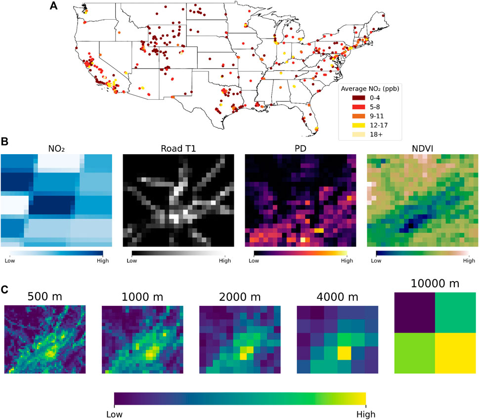
FIGURE 1. NO2 monitors and gridded variable representation examples. (A) Map of EPA NO2 monitors across the U.S. and their average NO2 concentrations over the study period. (B) Example gridded representations of the TROPOMI NO2, tier 1 (T1) roads, PD, and NDVI at the 1,000 m resolution. (C) Example data grid resolutions obtained from the ISA layer, ranging from 500 m to 10,000 m.
We excluded any monitoring data prior to July 2018, as the TROPOMI data was not yet available prior to that date. Daily averages were computed from the hourly data, and each daily average was considered to be valid if at least 75% of the day’s data was available (as following the EPA’s reliability criterion).
Although the COVID pandemic brought significant decreases in NO2 levels (Hoang et al., 2021) and certain studies (Larkin et al., 2023) excluding data after 2019 for that reason, we chose to include such data to provide the most up-to-date model for immediate NO2 predictions and to demonstrate the model’s capacity to adapt temporally to lurking factors.
Modeling variables and databases
The standard modeling variables were chosen from various commonly used satellite data methods used in past LUR approaches, such as traffic data, tree cover (TC), elevation (ELEV), and temperature (TP), with the full list of variables listed in Table 1. Traffic and railway (RW) data were obtained from the Open Street Map (OSM) database, a community based, worldwide map service widely used in many research applications (Vargas-Munoz et al., 2020). In this study, we used the OSMnx Python module to efficiently extract OSM information (Boeing et al., 2017).
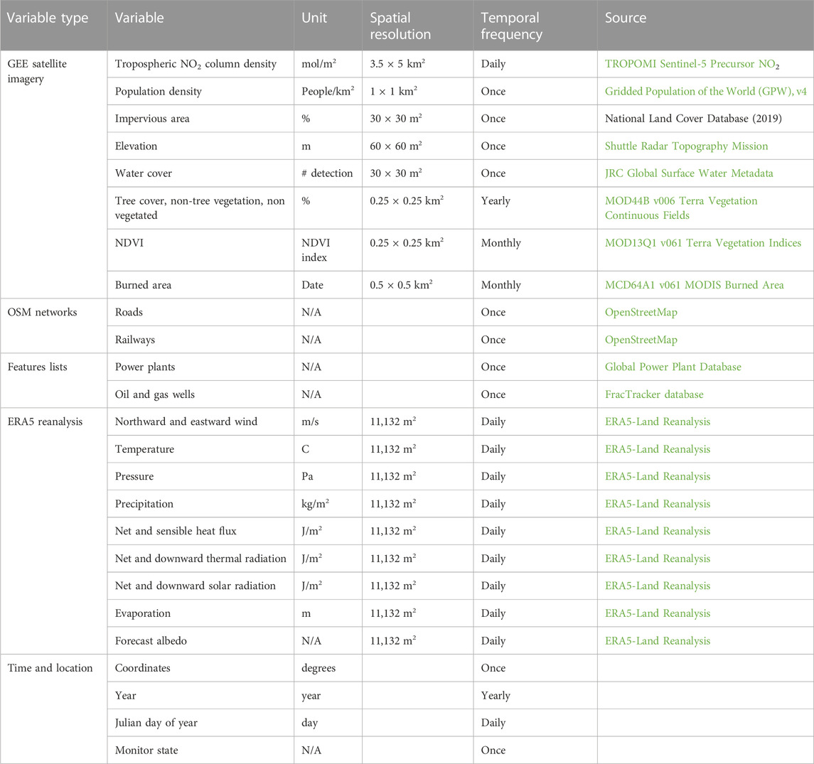
TABLE 1. All predictor variables (imagery and numerical) taken by the model. Temporal frequency indicates the frequency of data collected over the study period.
Almost the entirety of the satellite data and meteorological reanalysis, including the TROPOMI NO2, were obtained from the GEE database. The GEE database, a cloud computing platform which compiles a large set of satellite data into an easily accessible interface, greatly streamlines the data gathering process as the data of interest can be directly extracted without having to process entire datasets of raw data (Gorelick et al., 2017; Mutanga et al., 2019). GEE provides many built-in functions to obtain data in the needed format, working to streamline the preprocessing data collection to focus on the actual model development (Gorelick et al., 2017). Furthermore, GEE is also incredibly useful as its regularly updated cloud system allows satellite data of a given day at any location around the world to be easily extracted allowing immediate predictions. With GEE, we extracted the TROPOMI NO2 (Veefkind et al., 2012), population density (PD) (CISESIN, 2018), impervious surface area (ISA) (Dewitz et al., 2021), ELEV (Jarvis et al., 2008), water cover (WC) (Pekel et al., 2016), tree cover, non-tree vegetation (NTV), non-vegetated (NV) (DiMiceli et al., 2015), normalized difference vegetation index (NDVI) (Didan, 2021), and burned area (BA) (Giglio et al., 2021).
Oil and gas (O&G) wells, which also contribute to NO2 emissions, were also included in this study (Dix et al., 2022). O&G wells have generally been excluded from LUR studies, but the increasing prevalence of wells in the U.S. specifically potentially calls for their inclusion. Data of O&G wells was obtained from the FracTracker database, which gathers data of O&G wells from U.S. states (Jalbert et al., 2017). Lastly, power plants were obtained from the Global Power Plant Database. A full list of predictor variables leveraged by the model, their spatial resolutions, their temporal frequencies, and their sources is listed in Table 1.
Data grid representations
To represent each variable, we took advantage of the gridded format of the GIS data to directly pass it as a 2D image to the CNN. At a buffer distance of 10 km, each variable was represented as a pixel gridded image where each pixel represents the satellite measured value over the given region the pixel encompasses. 10 km is largely considered to be the maximum buffer distance for LUR studies, therefore it was considered to be our bounding box (Hoek et al., 2008; Novotny et al., 2011). Examples of selected gridded variable representations are displayed in Figure 1B.
Using the GEE database, data grids were computed based on each variable for each monitoring site. Three different scale resolutions were tested: 10,000 m, 4,000 m, 2,000 m, 1,000 m, and 500 m per pixel. Example plots of each size are displayed in Figure 1C. For the TROPOMI data, whose resolution is not as fine as the other variables, the original pixels were expanded to fit the size of the other variables. These computations were done using GEE’s scale computation involving image pyramids, which aggregates the data into various pyramidal scales and chooses the closest scale to the specified resolution. To ensure that each bounding box remains equal in size, we linearly interpolated each bounding box to fit the specified resolution. Due to much of the satellite data being gridded through latitude and longitude, bounding boxes were not entirely square for most resolutions.
Image plots of the road and railway networks were exported and resized to fit the pixel resolution of the satellite data using OSMnx. Road networks were separated into five separate tiers (Supplementary Table S1), with each passed as its own image. RW networks were given their own layer.
For power plants and O&G wells, which are datasets of features with coordinates rather than grids, empty data grids were first generated at a 10 km buffer distance. Then, each pixel was given a value based on the number of power plants or wells that were present in it and a zero if not. Oil (OP), gas (GP), coal (CP), and waste (WP) power plants were each given a layer, along with O&G wells.
The meteorological reanalysis data from the ERA5 global reanalysis dataset from GEE and was provided as averages over the 10 km buffer distance due to its coarse resolution (Munoz Sabater, 2019; Hersbach et al., 2020). In addition to regularly used meteorological variables including TP, wind components, precipitation (PC), evaporation (EV) and surface pressure (SP), we also included a couple of the ERA5 dataset’s other surface measurements including sensible/latent heat flux (SHF, LHF), normal/downward solar (SR, DSR) and thermal radiation (TR, TSR), and forecast albedo (FA). Wind components consisted of northward (VW) and eastward (UV), with their respective minimums and maximums. By providing a detailed assessment of meteorological variables, the model can better understand both atmospheric NO2 formation as well as seasonal variability in NO2 concentrations. Other non-image variables include the state of the monitor (one hot encoded), year of measurement, Julian day of the measurement, and lat-long coordinates of the monitor.
CNN model architecture
In this study, the widely successful CNN was applied to learn from the spatial patterns of the satellite generated pixel gridded images. CNNs are a class of neural networks that scan through a given input image with various filters to extract important features (LeCun et al., 2015; O’Shea and Nash, 2015). Then, these features are processed in a feed forward fashion to generate predictions.
In this task where multiple “images” are provided as input, there are three potential architectures of varying complexity to leverage. The first architecture consists of stacking each of the images together to form a multi-channel, 3D tensor, and train using four 2D convolution layers.
The second architecture treats the images like a video, with each image variable contained in its own 3D tensor. Each 3D tensor is then combined into a single 4D tensor, in which 3D convolution layers are used rather than 2D layers. Figure 2A displays a model of architectures 1 and 2.
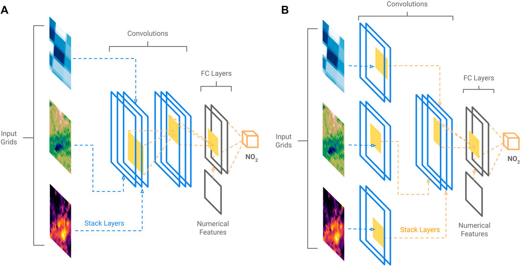
FIGURE 2. CNN model architectures 1 and 2 (A), which stack layers prior to applying convolutions, and architecture 3 (B), which first apply convolutions to each layer before stacking and applying further convolutions.
The final, more complex architecture similarly treats each image as its own 3D tensor. However, instead of stacking the data into a 4D tensor, two unique convolution layers first process each image variable before the information is passed into the last three convolution layers, as Kappeler et al. (2016) introduced in their video processing CNN (Figure 2B).
Lastly, the numerical features are concatenated to the fully-connected (FC) layer at the end of the convolutions before going through two more FC layers to generate the prediction with rectified linear unit (ReLU) initializers to introduce nonlinearity (Nair and Hinton, 2010), as well as dropout layers to combat overfitting (Srivastava et al., 2014). All modeling was conducted using the PyTorch module in Python and a NVIDIA RTX A4000 GPU (Paszke et al., 2019).
Buffer distance models
In addition to the CNN, we also developed various buffer distance models using three buffers of 1 km, 5 km, and 10 km to directly compare with the CNN. Each variable that was once represented as an image was computed into those three buffer distance averages. Using that dataset, we trained a feedforward neural network (FNN), a random forest (RF) model, as well as a classic multivariate linear regression (MLR) for both daily and annual prediction tasks.
The FNN is a network of neuron layers, where the neurons of each layer are connected to every neuron of the next layer through a weight coefficient, thus resulting in a 2D matrix of weights to transform the representations at each layer (Svozil et al., 1996). Ultimately, we built a three layer FNN using a hidden layer of 128 neurons with the PyTorch module in Python (Paszke et al., 2019), as three layer networks show sufficiently capable prediction ability (Eldan and Shamir, 2016). Between each layer, we used the ReLU activation function, which introduces nonlinearity within the network (Nair and Hinton, 2010), as well as dropout layers to combat overfitting (Srivastava et al., 2014). Lastly, using the backpropagation algorithm given by stochastic gradient descent (SGD), the weight matrices are optimized to best predict the output variable, being the NO2 measurement (Bottou, 2012).
Next, we also developed an RF model, which is a set of several individual decision trees whose results are combined to form the culminating RF’s prediction (Breiman, 2001). Each decision tree is built through a network of if-then-else branches that are split using a scoring criterion, such as Gini for classification and mean squared error for regression (Myles et al., 2004). We developed our RF model in the Scikit-Learn Python module using the RandomForestRegressor class with 200 decision trees (Pedregosa et al., 2011). For each decision tree, after resampling from the training data, we use log2 times the number of features to build each split that best minimizes the mean squared error. Then, the resulting values from each decision tree are averaged to obtain the RF’s NO2 prediction.
Lastly, we implemented a classic MLR model, which simply aims to fit the coefficients of a linear model that minimizes the residual sum of squares between observed and predicted values (Alexopoulos, 2010). We similarly implemented the MLR using the LinearRegression class in Scikit-Learn (Pedregosa et al., 2011).
Model analysis
To analyze the performance of each CNN, we performed a 10-fold cross validation (CV). Using the entire dataset of all monitoring sites and their measurements, we separated the data into ten different chunks, training the model on nine chunks and evaluating on the final chunk in ten separate iterations. Three metrics were used for this evaluation: the coefficient of determination (R2), root mean squared error (RMSE), and mean absolute error (MAE).
In addition to the 10-fold CV, a spatial and temporal hold-out validation was also conducted. The spatial evaluation separates the list of monitoring sites into ten separate chunks. Then, the model is trained on the measurements of the monitoring sites of nine chunks and evaluated on the measurements of the sites of the final chunk in ten separate iterations. The temporal evaluation holds out each year of data for evaluation, and trains the model on the other years between 2018–2022 for each year in the analysis. The spatial evaluation simulates using the model to predict for unseen locations, and the temporal evaluation simulates the model predicting for future/past years. Example scripts used in this study can be found at the following Github repository: https://github.com/eltonc01/national-no2-cnn.
Results and discussion
Model input overview
From the 500 monitoring sites across the contiguous US, we obtained 234,781 daily averages and 1,350 annual averages over the 4 year study period. After 2020, due to the COVID pandemic, there was a marked decrease in average NO2 measurements, decreasing from 8.08 ppb pre-2020 to 7.59 ppb 2020 and beyond (p < 0.001).
Between the image resolutions of 500 m, 1,000 m, 2,000 m, 4,000 m, and 10,000 m, we obtained data grids of size 42 × 50, 20 × 24, 10 × 12, 5 × 6, and 2 × 2 respectively using Google Earth Engine’s scale computation. Example data grids of these resolutions are shown in Figure 1C.
Model architecture and resolution selection results
Using the image resolutions, we trained the three model architectures to both ascertain the effect of image resolution on CNN performance and identify the most efficient model by comparing model performance.
Between the three architectures, there was not a significant difference between each model’s performance. Architectures 1 and 2 comparing 2D and 3D convolution layers respectively achieved similar performance (Supplementary Figure S1). Additionally, the more complex architecture 3 did not provide a boost in performance despite greater computational resources consumed. We opted for architecture 1 due to its simplicity throughout the study.
Interestingly, image resolution similarly did not improve model performance. For the daily model, between the resolutions of 500 m (daily R2: 0.879; annual R2: 0.951), 1,000 m (daily R2: 0.885; annual R2: 0.947), 2,000 m (daily R2: 0.889; annual R2: 0.950) and 4,000 m (daily R2: 0.892; annual R2: 0.952), each model’s R2 indicated similar performance, with higher resolution inputs even showing a slight decrease in R2 performance, especially in the daily models (Figure 3A, Supplementary Table S2). Additionally, the 10,000 m resolution model, which was simply just a 2 × 2 grid, similarly performed fairly well (daily R2: 0.877; annual R2: 0.937), albeit slightly worse than the higher resolutions. These results suggest that the CNN does not require a high resolution to maintain its accuracy; in fact, it may benefit more from a more generalized and less nuanced input. Although many deep learning tasks may require large and complex models to train such as certain image recognition tasks accomplished using ResNet models (Allen-Zhu and Li, 2019), we demonstrate that the task of NO2 prediction can be successfully done with simple, from-scratch CNN models.
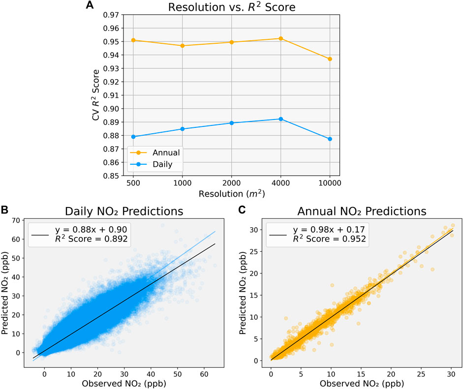
FIGURE 3. CNN satellite data resolution and performance. (A) CNN satellite data resolution vs 10-fold CV R2 score for daily (blue) and annual (yellow) prediction tasks. (B + C) Observed NO2 vs CNN predicted NO2 concentrations for daily (B) and annual (C).
The architectures and resolution indicate that the problem does not need particularly complex machine learning inputs, with low resolution images and simple CNN architectures achieving the best and most efficient performance. With these low resolution images and simpler architectures, models can be trained and developed at a much faster rate.
Furthermore, it was only when restricting the image resolution to a very coarse 10,000 m per pixel that the TROPOMI NO2 data had to be blurred from its input size. Since a decrease in performance was observed in the only iteration where the NO2 grid resolution was decreased, it suggests that the CNN relies largely on the TROPOMI data. However, when evaluating on a model which did not include the TROPOMI data, the CNN only experienced a slight drop in performance (daily R2: 0.873; annual R2: 0.939), albeit the model took notably longer to converge and more epochs to train (Supplementary Table S3).
When taking the best performing resolution of 4,000 m and the simplest architecture 1, we obtained a daily 10-fold CV R2 score of 0.892, RMSE of 2.259, and MAE of 1.534 and an annual 10-fold CV R2 score of 0.952, RMSE of 0.988, and MAE of 0.690. When comparing the observed vs the predicted NO2 concentrations, both models achieve a high correlation (Figures 3B, C).
Model and method comparison
We also developed a set of buffer distance-based models to directly compare the CNN’s 2D representation with the classic approach of providing various buffer distance averages. Among those models, we developed FNN, RF, and MLR models using 1 km, 5 km, and 10 km buffers. These models represent the simplest buffer distance based models, using both nonlinear and linear statistical models, so that it is possible to gauge the effect of model type on air quality prediction given that each model uses the same predictor variables.
Out of all the models, the MLR performed poorest (daily R2: 0.625, annual R2: 0.758), indicating that linear approaches are likely too simple to quantify NO2 concentrations. This result is consistent with past implementations of linear models, and despite its fastest computational time, the linear dependencies between the GIS predictor variables likely cannot capture the complexities behind NO2 prediction (Ghahremanloo et al., 2021; Kang et al., 2021).
The FNN makes a significant improvement in performance compared to the MLR (daily R2: 0.863, annual R2: 0.863). The FNN, which leveraged a 2D matrix of weights, rather than a 1D vector of weights in the MLR, and a nonlinear activation function, provided the necessary nonlinearity to the buffer distance GIS predictor variables towards greatly improved NO2 predictions (Maas et al., 2013). Similarly, the RF also shows a significant improvement from the MLR (daily R2: 0.863, annual R2: 0.828). RF models, which are made up of a large number of decision trees, are similarly able to capture nonlinearity within the GIS predictor variables. Each decision tree makes a network of if-then-else branches, and with hundreds of these deep decision tree networks, the RF captures a significant portion of nonlinear patterns within the data to ultimately increase predictive capacity (Biau and Scornet, 2016).
Between all models developed in this study, the CNN performed best in all metrics, providing further improvements on the FNN and RF approaches (Table 2; Supplementary Figure S2). The CNN gains much of the advantages provided by the FNN, with deeper weight matrices and nonlinear activation functions. However, with the more informative 2D representation leveraged by the CNN’s approach, the model can likely better learn specific factors which lead to ground-level NO2 concentrations at a given site. With the CNN’s backpropagation boosted filters, the most predictive properties of the buffer region are automatically identified and purposed towards prediction, hence the feature extraction of the CNN, which is the primary mechanism behind CNNs success (Jogin et al., 2018). Rather than simply forcing the model to predict using a set of predefined buffer averages, the CNN has freedom to select which spatial patterns in the GIS variables it deems to be important and use those towards NO2 prediction.
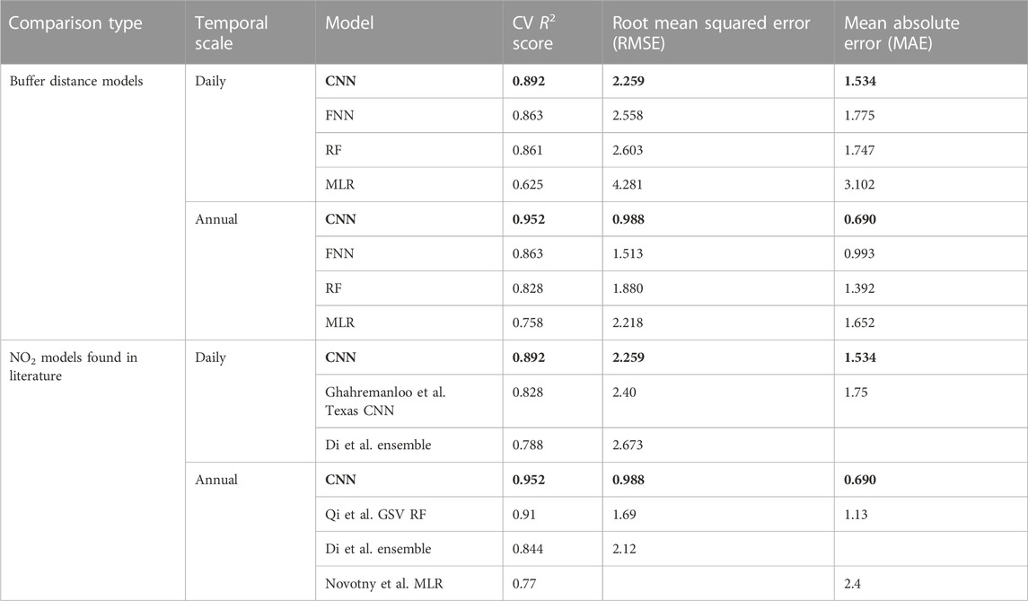
TABLE 2. CNN performance compared to buffer distance models and models found in literature for both daily and annual temporal scales. Bolded values indicate the best performing model’s metric in each section.
In regards to computational training time, each model trained did not require intense computational resources. Due to the lower resolution imagery, model training was quick even for the more complex CNN. Although FNN, RF, and MLR approaches were much faster to train in comparison, the overall training time required by the CNN was not particularly intense, maintaining the lower cost of developing statistical models over computationally heavy physical chemical transport models.
Compared to national NO2 models in literature, the CNN achieves highly competitive performance, improving metric-wise on Ghahremanloo et al.‘s Texas CNN, Di et al.‘s ensemble, and Novotny et al.‘s MLR, which are based on buffer distances. Developing effective models for expansive regions, such as the contiguous U.S. or even the state of Texas, can be difficult with many LUR models optimized for districts or cities. However, the CNN regardless displays a very high accuracy in predicting NO2. Furthermore, despite the success of Qi et al.‘s novel GSV image approach, the CNN regardless maintains increased performance while using classic land use GIS variables. Although some of this effect could potentially be attributed to the CNN using the more detailed TROPOMI data (Qi et al. used the coarser OMI data) and our model being trained on a smaller timespan, our results still indicate the strengths of using land use variables in a more detailed way.
It can be difficult to accurately compare model performances between models from different studies. However, these results mirror the results comparing the CNN to our own buffer distance models, ultimately suggesting that the novel CNN 2D representation approach has strengths over classic buffer distance approaches.
Spatial and temporal CVs
In addition to the 10-fold CVs, we also conducted a spatial and temporal CV to test the CNNs ability to predict for both unseen locations and unseen years. In the spatial evaluation, model performance dropped significantly, with a daily R2 CV score of 0.593 and an annual R2 CV score of 0.549 (Supplementary Table S4). This result is consistent with many other LUR models, indicating that the issue of a lower spatial evaluation performance has yet to be solved (Park et al., 2020; Ghahremanloo et al., 2021; Qi et al., 2022).
For the temporal evaluation, it is not only important to consider the overall accuracy, but also whether the hold-out temporal year is within the range of years trained or if we are extrapolating for past or future years. Overall, both daily and annual models experienced a slight drop in performance, with a daily R2 CV score of 0.848 and an annual R2 CV score of 0.943 (Supplementary Table S5). Regarding the daily model, when we did not extrapolate temporally (years 2019–2021), the CNN recorded an average R2 score of 0.854. However, when extrapolating, performance dropped slightly to R2 score of 0.838 (2018) and 0.839 (2022). Annually, a slightly differing pattern was observed. Extrapolating for a past year did not decrease performance; however, when extrapolating for a future year, R2 score dropped to 0.929.
A factor weighing into the poorer performance for both the spatial and temporal evaluations could also be the smaller timespan. With more years to train on, the model can likely better ascertain the effect of changing years regarding the temporal evaluation, and more samples of the changing landscapes over time provide different types of spatial factors for the model to learn from a more diverse set of locations.
Time series analysis
We also evaluated our model in a time series forecasting scenario, where the model is trained on years 2018–2021 and attempts to forecast the year 2022. Although our model was not developed as a forecasting model, with recurrent neural networks (RNN) better suited to the task (Tsai et al., 2018), it is regardless useful to identify the model’s predictive capacity in this scenario, and how well a statistical model could potentially replace a real NO2 monitor.
We first individually evaluated the MAE of each specific monitoring site when forecasting for 2022, with Figure 4A displaying a histogram of the MAEs of each site. Although there are certain sites where the model predicts poorly, the model overall displays a decent distribution of performance.
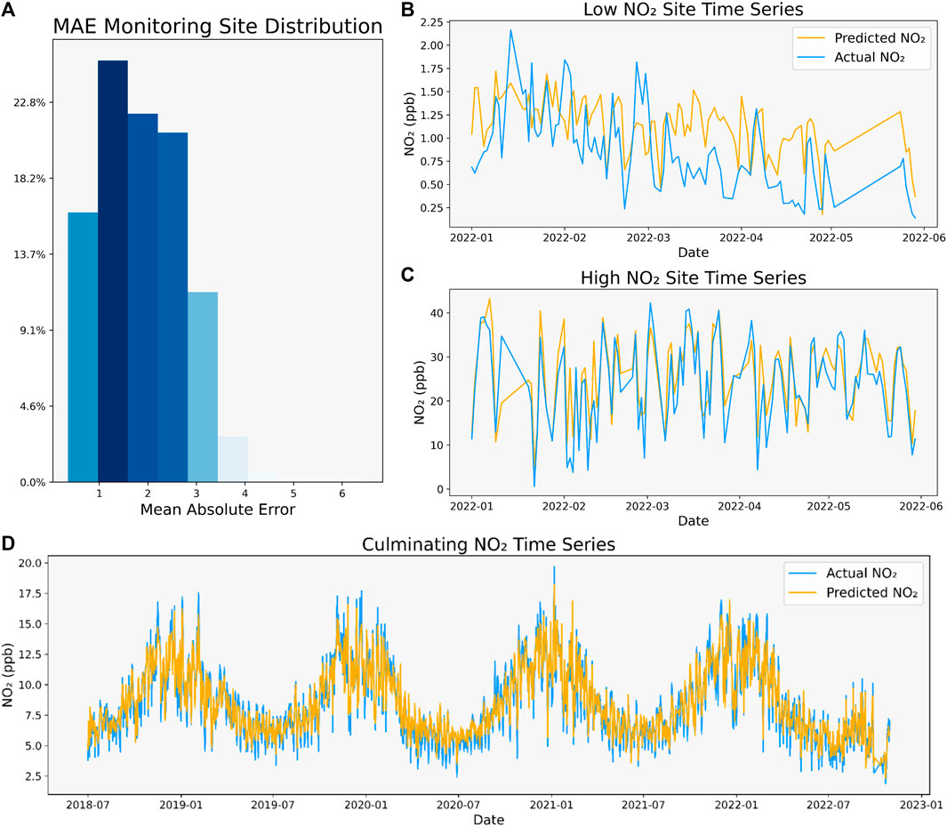
FIGURE 4. CNN time series analysis. (A) Histogram of MAE scores individual to each monitoring site. (B + C) Predicted and actual time series over 2022 for low (B) and high (C) NO2 monitors. (D) Culminating NO2 time series with all monitors over the entire study period.
Additionally, we also selected two specific monitors to investigate their time series prediction for 2022. We chose two monitors to conduct the analysis: one monitor in a low NO2 environment, and another in a high NO2 environment. Both monitors were from California, with the high NO2 monitor located at the coordinates (34.068120°, −117.525790°) outside Los Angeles located near an interstate highway, and the low NO2 monitor located at the coordinates (34.725352°, −120.428717°) in the rural region between the coastline of Los Angeles and San Francisco (Supplementary Figure S3).
Figures 4B, C display the predicted and actual time series for both specific monitors. The prediction model had difficulty in capturing the variance in the low NO2 environment, only capturing the general trend. This suggests the model has difficulty capturing very fine variances in NO2 concentrations. Compared to the high NO2 environment, the model appears to capture larger scale variances in NO2 concentrations, with the predicted time series matching the actual time series closely.
Although the model was also not optimized to predicting time series, the model regardless displayed fairly good performance for predicting NO2 time series. Models optimized to predicting time series are often built using RNNs, which incorporate past NO2 concentrations to infer the concentration of the next time step (Tsai et al., 2018). Although our model lacked this “past” information and leveraged the spatial information only, it regardless matched the actual time series well.
Lastly, we also analyzed the overall time series patterns in Figure 4D, which displays the actual and predicted overall time series by averaging the predictions of all monitoring sites of each day across the entire study period. In the actual time series, the seasonal variability of NO2 concentrations appears in peaks over winter seasons and lows over summer seasons. The CNN’s predicted time series closely matches this seasonal variation, indicating the model’s ability to understand seasonal variations in NO2 concentrations. Given Julian day and other meteorological variables such as temperature, the model gains an understanding of the distinct seasons. Considering anthropogenic, biomass burning, and soil emissions as the primary sources of NO2 seasonal variability (Van Der A et al., 2008), our model can use the variable indicators of those sources (ex: ISA, BA, and NDVI respectively) combined with seasonal understanding to identify contributors to seasonal variation in NO2. In the U.S., anthropogenic sources contribute most towards seasonal variability in NO2, which our model thoroughly assessed through various road, RW, ISA, and PD variables (Van Der A et al., 2008). Furthermore, given a thorough meteorological assessment of variables such as solar radiation, which contribute to seasonal NO2 atmospheric lifetime, the CNN effectively understands meteorological parameters contributing to seasonal variability (Van Der A et al., 2008).
SHAP analysis
Using the SHAPely Additive Explanations (SHAP), many once black-box deep learning models could be effectively interpreted, including CNNs (Lundberg et al., 2017). SHAP analyzes each individual prediction and determines what features factored into making the prediction by comparing the model predictions with and without the feature. To determine the importance and effect of each feature on the CNNs predictions, we ran a SHAP analysis to determine the individual effects of each variable on model performance, as well as how the CNN processes each data grid for prediction.
We first ran a general SHAP analysis by gathering the effects of the pixels of each variable together into a plot. A larger SHAP value indicates a greater feature importance for a given prediction. For each GIS variable grid, we summed up all the SHAP and actual pixel values in a grid to compare with the numerical variables. Additionally, due to the removal of the TROPOMI having a minimal effect on performance, we ran SHAP analysis for both a TROPOMI CNN model and a TROPOMI-less CNN model. We chose to only analyze the annual model to allow SHAP to better generalize to the dataset with a more encompassing set of background samples in a reasonable span of time, as having a large number of background samples reduces the variability of the results (Yuan et al., 2022).
In the general SHAP analysis described in Figure 5A, the model favored many variables that were previously identified as important in past LUR models, such as the road variables (positive correlation) and NDVI (negative correlation). Similarly, many of the more detailed meteorological variables, such as thermal radiation, were identified as important features in the model. Considering the role that atmospheric and meteorological variables play in NO2 formation, these results indicate the CNN began to identify chemical processes of NO2 formation (Atkinson, 2000; Voiculescu et al., 2020).
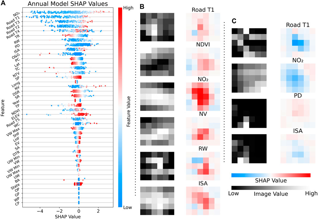
FIGURE 5. CNN SHAP analysis. (A) General SHAP analysis for annual NO2 predictions. The x-axis lists SHAP values, while the y-axis lists the features. Each point represents the SHAP values from an individual prediction, with the scale on the right indicating the real value of the feature. (B + C) Singular SHAP analysis for urban (B) and rural (C) monitoring sites. The right row of these figures is the plot of SHAP values for each pixel in the grid, and the left row is the actual pixel grid, with white values indicating a higher value and black values indicating a lower value.
However, although the TROPOMI NO2 was identified as the most important feature in the annual analysis, its removal had a minimal impact on overall model performance for both daily and annual models. In the SHAP analysis of the TROPOMI-less model, the model’s feature importance did not change significantly; rather, it used the same features to compensate for the lack of TROPOMI information (Supplementary Figure S4). While previous buffer distance LUR models relied heavily on the TROPOMI information (Novotny et al., 2011), our model was only slightly impacted, further indicating the strength of providing a 2D CNN representation as opposed to the classic buffer distance method.
Interestingly, O&G wells were identified as an important feature by the SHAP analysis. However, the numbers corresponding to the SHAP values do not quite indicate that more O&G wells influences higher NO2. Regardless, O&G wells should likely be useful to include in future LUR models due to their importance here.
Lastly, we also conducted a more focused SHAP analysis using the annual model by selecting specific monitoring sites and analyzing the spread of SHAP values within the data grids of certain important variables. For this singular analysis, we chose the two monitors used in the previous time series analysis: one in a high NO2 and another in a low NO2 environment, which allow the factors contributing to NO2 to be more clearly observed. The high NO2 monitor recorded an average NO2 concentration of 29.89 ppb and the low monitor 0.35 ppb over the study period. For both samples, we chose the most recent year of 2021, in which the urban monitor recorded a concentration of 29.04 ppb and the rural 0.49 ppb. For the urban monitor, the model predicted a concentration of 29.31 ppb, and for the rural monitor, the model predicted a concentration of 0.41 ppb.
In Figure 5, we displayed a set of notable variable layers from the urban (Figure 5B) and rural (Figure 5C) analyses. Within both samples, the model’s filters learned to quantify pixels near the center of the plot as more important due to proximity to the monitor. For example, in the rural Road Tier 1 (T1) and ISA layers, the absence of roads and impervious % in the middle of the plot resulted in a decrease in SHAP values. In the urban analysis, the presence of roads and rails near the middle of the plot showed larger SHAP values.
Conversely, the model also learned to take the pixels near the edge of the plot with less consideration. For example, despite the Road T1 plot for the rural monitor being influenced by a highway near the top, it contributed little to the overall SHAP analysis.
Among both analyses, the NO2 layer continues to contribute a large amount of SHAP values. Furthermore, these NO2 SHAP values seemed to appear in spreads of SHAP values rather than individual peaks. The actual NO2 values may not necessarily be lower/higher, but if the overall spread of NO2 was generally low/high, the whole region would contribute to the SHAP value in the same direction.
Limitations and future implications
In this study, we built a novel NO2 LUR model based on satellite GIS variables in a novel CNN pixel plot representation for both daily and annual temporal scales. By representing these GIS variables in a pixel plot, more detailed features can be learned by the model to make its predictions.
The primary limitation behind the CNN lies in its poor spatial evaluation performance. However, this limitation is not experienced by the CNN alone; in fact, this is an issue observed in statistical models in general, as they are often confined to the specific regions they are trained on. Compared to advanced physical models, which develop a set of comprehensive patterns that can account for a broad set of environments, statistical models face a major limitation.
Such an issue can likely not be solved by model architecture alone, as the problem likely lies in the inherent lack of monitoring sites. With more monitoring sites and diverse locations, models like the CNN can learn better about what types/formations of surroundings that would lead to a given NO2 concentration. Due to the lack of this general diversity, an unseen location is interpreted as completely novel by the model as it has never seen any sample similar to the location, thereby resulting in poor predictive capacity. As methods of mobile monitoring (Padilla et al., 2022) and low-cost sensors (van Zoest et al., 2019) advance and diffuse across the U.S., we expect the CNN along with LUR models in general to improve significantly for the prediction of unseen locations.
Furthermore, with the recent launch of the new TEMPO satellite (Zoogman et al., 2017), which provides higher resolution NO2 imagery over North America only thereby providing more frequent measurements, the CNN could improve both in its general performance and its spatial validations. Satellite NO2 remains a fairly good predictor of ground-level NO2 regardless of whether a location has been seen or not, therefore higher quality data would likely benefit the model’s spatial prediction ability (Goldberg et al., 2021).
In the future, this approach could also potentially be expanded beyond the contiguous U.S. With the model only requiring coarse resolution imagery to achieve excellent performance, the entire world could be quickly mapped using the readily available GIS satellite data. Although this approach has not been tested outside of the U.S., it has adapted well to state-to-state variations in NO2 and can likely show the same performance globally.
Conclusion
In this study, using GIS satellite imagery, meteorological reanalysis, and TROPOMI tropospheric NO2 data, we developed a CNN which inputs a 2D buffer representation towards more comprehensive NO2 predictions. Using the same predictor variables, we also developed FNN, RF, and MLR models based on 1D buffer distance averages. Among these models, the CNN outperformed buffer distance models and past NO2 LUR methods. Using the GEE database, the once tedious data collection process from various data sources was optimized into an efficient pipeline that allows immediate predictions to be made by the model. With the CNN, we hope to provide more accurate and precise NO2 monitoring across the contiguous U.S. As modern deep learning frameworks continue to develop, we expect to see their rapid implementation in this field with the success of CNNs in this study.
Data availability statement
The original contributions presented in the study are included in the article/Supplementary Material, further inquiries can be directed to the corresponding author.
Author contributions
EC: Conceptualization, Data curation, Formal Analysis, Investigation, Methodology, Software, Writing–original draft, Writing–review and editing.
Funding
The author(s) declare that no financial support was received for the research, authorship, and/or publication of this article.
Acknowledgments
We would like to thank Paul K. Strode for his important guidance throughout the authors’ research careers.
Conflict of interest
The author declares that the research was conducted in the absence of any commercial or financial relationships that could be construed as a potential conflict of interest.
Publisher’s note
All claims expressed in this article are solely those of the authors and do not necessarily represent those of their affiliated organizations, or those of the publisher, the editors and the reviewers. Any product that may be evaluated in this article, or claim that may be made by its manufacturer, is not guaranteed or endorsed by the publisher.
Supplementary material
The Supplementary Material for this article can be found online at: https://www.frontiersin.org/articles/10.3389/fenvs.2023.1285471/full#supplementary-material
References
Alexopoulos, E. C. (2010). Introduction to multivariate regression analysis. Hippokratia 14 (Suppl. 1), 23–28.
Allen-Zhu, Z., and Li, Y. (2019). What can resnet learn efficiently, going beyond kernels? Adv. Neural Inf. Process. Syst. 32.
Atkinson, R. (2000). Atmospheric chemistry of VOCs and NOx. Atmos. Environ. 34 (12-14), 2063–2101. doi:10.1016/s1352-2310(99)00460-4
Biau, G., and Scornet, E. (2016). A random forest guided tour. Test 25, 197–227. doi:10.1007/s11749-016-0481-7
Boeing, G. (2017). OSMnx: new methods for acquiring, constructing, analyzing, and visualizing complex street networks. Comput. Environ. Urban Syst. 65, 126–139. doi:10.1016/j.compenvurbsys.2017.05.004
Bottou, L. (2012). “Stochastic gradient descent tricks,” in Neural networks: tricks of the trade (Berlin, Germany: Springer), 421–436.
Byun, D., and Schere, K. L. (2006). Review of the governing equations, computational algorithms, and other components of the Models-3 Community Multiscale Air Quality (CMAQ) modeling system. Appl. Mech. Rev. 59 (2), 51–77. doi:10.1115/1.2128636
Center for International Earth Science Information Network - CIESIN - Columbia University (2018). Gridded population of the world, version 4 (GPWv4): population density, revision 11. Palisades, NY, USA: NASA Socioeconomic Data and Applications Center SEDAC. doi:10.7927/H49C6VHW
Chan, K. L., Khorsandi, E., Liu, S., Baier, F., and Valks, P. (2021). Estimation of surface NO2 concentrations over Germany from TROPOMI satellite observations using a machine learning method. Remote Sens. 13 (5), 969. doi:10.3390/rs13050969
Chiusolo, M., Cadum, E., Stafoggia, M., Galassi, C., Berti, G., Faustini, A., et al. (2011). Short-term effects of nitrogen dioxide on mortality and susceptibility factors in 10 Italian cities: the EpiAir study. Environ. Health Perspect. 119 (9), 1233–1238. doi:10.1289/ehp.1002904
Clark, L. P., Millet, D. B., and Marshall, J. D. (2014). National patterns in environmental injustice and inequality: outdoor NO2 air pollution in the United States. PloS One 9 (4), e94431. doi:10.1371/journal.pone.0094431
Costa, S., Ferreira, J., Silveira, C., Costa, C., Lopes, D., Relvas, H., et al. (2014). Integrating health on air quality assessment—review report on health risks of two major European outdoor air pollutants: PM and NO2. J. Toxicol. Environ. Health, Part B 17 (6), 307–340. doi:10.1080/10937404.2014.946164
De Hoogh, K., Saucy, A., Shtein, A., Schwartz, J., West, E. A., Strassmann, A., et al. (2019). Predicting fine-scale daily NO2 for 2005–2016 incorporating OMI satellite data across Switzerland. Environ. Sci. Technol. 53 (17), 10279–10287. doi:10.1021/acs.est.9b03107
De Hoogh, K., Wang, M., Adam, M., Badaloni, C., Beelen, R., Birk, M., et al. (2013). Development of land use regression models for particle composition in twenty study areas in Europe. Environ. Sci. Technol. 47 (11), 5778–5786. doi:10.1021/es400156t
Di, Q., Amini, H., Shi, L., Kloog, I., Silvern, R., Kelly, J., et al. (2019). Assessing NO2 concentration and model uncertainty with high spatiotemporal resolution across the contiguous United States using ensemble model averaging. Environ. Sci. Technol. 54 (3), 1372–1384. doi:10.1021/acs.est.9b03358
Dickerson, R. R., Anderson, D. C., and Ren, X. (2019). On the use of data from commercial NOx analyzers for air pollution studies. Atmos. Environ. 214, 116873. doi:10.1016/j.atmosenv.2019.116873
Didan, K. (2021). MODIS/Terra vegetation indices 16-day L3 global 250m SIN grid V061. NASA EOSDIS Land Process. DAAC. doi:10.5067/MODIS/MOD13Q1.061
DiMiceli, C., Carroll, M., Sohlberg, R., Kim, D., Kelly, M., and Townshend, J. (2015). MOD44B MODIS/terra vegetation continuous fields yearly L3 global 250m SIN grid V006. NASA EOSDIS Land Process. DAAC. doi:10.5067/MODIS/MOD44B.006
Dix, B., Francoeur, C., Li, M., Serrano-Calvo, R., Levelt, P. F., Veefkind, J. P., et al. (2022). Quantifying NOx emissions from U.S. Oil and gas production regions using TROPOMI NO2. ACS Earth Space Chem. 6 (2), 403–414. doi:10.1021/acsearthspacechem.1c00387
Eldan, R., and Shamir, O. (2016). The power of depth for feedforward neural networks. https://arxiv.org/abs/1512.03965.
Finazzi, F., Scott, E. M., and Fassò, A. (2013). A model-based framework for air quality indices and population risk evaluation, with an application to the analysis of Scottish air quality data. J. R. Stat. Soc. Ser. C Appl. Statistics 62 (2), 287–308. doi:10.1111/rssc.12001
Gbd Risk Factors Collaborators, , Afshin, A., Abajobir, A. A., Abate, K. H., Abbafati, C., Abbas, K. M., et al. (2017). Global, regional, and national comparative risk assessment of 84 behavioural, environmental and occupational, and metabolic risks or clusters of risks, 1990–2016: a systematic analysis for the Global Burden of Disease Study 2016. Lancet 390 (10100), 1345–1422. doi:10.1016/s0140-6736(17)32366-8
Ghahremanloo, M., Lops, Y., Choi, Y., and Yeganeh, B. (2021). Deep learning estimation of daily ground-level NO2 concentrations from remote sensing data. J. Geophys. Res. Atmos. 126 (21), e2021JD034925. doi:10.1029/2021jd034925
Giglio, L., Justice, C., Boschetti, L., and Roy, D. (2021). MODIS/Terra+Aqua burned area monthly L3 global 500m SIN grid V061. NASA EOSDIS Land Process. DAAC. doi:10.5067/MODIS/MCD64A1.061
Goldberg, D. L., Anenberg, S. C., Kerr, G. H., Mohegh, A., Lu, Z., and Streets, D. G. (2021). TROPOMI NO2 in the United States: a detailed look at the annual averages, weekly cycles, effects of temperature, and correlation with surface NO2 concentrations. Earth's Future 9 (4), e2020EF001665. doi:10.1029/2020ef001665
Gorelick, N., Hancher, M., Dixon, M., Ilyushchenko, S., Thau, D., and Moore, R. (2017). Google earth engine: planetary-scale geospatial analysis for everyone. Remote Sens. Environ. 202, 18–27. doi:10.1016/j.rse.2017.06.031
Greenberg, N., Carel, R. S., Derazne, E., Bibi, H., Shpriz, M., Tzur, D., et al. (2016). Different effects of long-term exposures to SO2 and NO2 air pollutants on asthma severity in young adults. J. Toxicol. Environ. Health, Part A 79 (8), 342–351. doi:10.1080/15287394.2016.1153548
Gu, J., Wang, Z., Kuen, J., Ma, L., Shahroudy, A., Shuai, B., et al. (2018). Recent advances in convolutional neural networks. Pattern Recognit. 77, 354–377. doi:10.1016/j.patcog.2017.10.013
Hersbach, H., Bell, B., Berrisford, P., Hirahara, S., Horányi, A., Muñoz-Sabater, J., et al. (2020). The ERA5 global reanalysis. Q. J. R. Meteorological Soc. 146 (730), 1999–2049. doi:10.1002/qj.3803
Hoang, A. T., Huynh, T. T., Nguyen, X. P., Nguyen, T. K. T., and Le, T. H. (2021). An analysis and review on the global NO2 emission during lockdowns in COVID-19 period. Energy Sources, Part A Recovery, Util. Environ. Eff., 1–21. doi:10.1080/15567036.2021.1902431
Hoek, G., Beelen, R., De Hoogh, K., Vienneau, D., Gulliver, J., Fischer, P., et al. (2008). A review of land-use regression models to assess spatial variation of outdoor air pollution. Atmos. Environ. 42 (33), 7561–7578. doi:10.1016/j.atmosenv.2008.05.057
Ialongo, I., Virta, H., Eskes, H., Hovila, J., and Douros, J. (2020). Comparison of TROPOMI/Sentinel-5 Precursor NO&lt;sub&gt;2&lt;/sub&gt; observations with ground-based measurements in Helsinki. Atmos. Meas. Tech. 13 (1), 205–218. doi:10.5194/amt-13-205-2020
Jalbert, K., Rubright, S. M., and Edelstein, K. (2017). The civic informatics of FracTracker Alliance: working with communities to understand the unconventional oil and gas industry. Engaging Sci. Technol. Soc. 3, 528–559. doi:10.17351/ests2017.128
Jarvis, A., Reuter, H. I., Nelson, A., and Guevara, E. (2008). Hole-filled SRTM for the globe version 4, available from the CGIAR-CSI SRTM 90m database. https://srtm.csi.cgiar.org.
Jogin, M., Madhulika, M. S., Divya, G. D., Meghana, R. K., and Apoorva, S. (2018). “Feature extraction using convolution neural networks (CNN) and deep learning,” in 2018 3rd IEEE international conference on recent trends in electronics, information & communication technology (RTEICT), Banglore, India, May, 2018, 2319–2323.
Kaminski, J. W., Neary, L., Struzewska, J., McConnell, J. C., Lupu, A., Jarosz, J., et al. (2008). GEM-AQ, an on-line global multiscale chemical weather modelling system: model description and evaluation of gas phase chemistry processes. Atmos. Chem. Phys. 8 (12), 3255–3281. doi:10.5194/acp-8-3255-2008
Kang, G. K., Gao, J. Z., Chiao, S., Lu, S., and Xie, G. (2018). Air quality prediction: Big data and machine learning approaches. Int. J. Environ. Sci. Dev. 9 (1), 8–16. doi:10.18178/ijesd.2018.9.1.1066
Kang, Y., Choi, H., Im, J., Park, S., Shin, M., Song, C. K., et al. (2021). Estimation of surface-level NO2 and O3 concentrations using TROPOMI data and machine learning over East Asia. Environ. Pollut. 288, 117711. doi:10.1016/j.envpol.2021.117711
Kappeler, A., Yoo, S., Dai, Q., and Katsaggelos, A. K. (2016). Video super-resolution with convolutional neural networks. IEEE Trans. Comput. Imaging 2 (2), 109–122. doi:10.1109/tci.2016.2532323
Knibbs, L. D., Hewson, M. G., Bechle, M. J., Marshall, J. D., and Barnett, A. G. (2014). A national satellite-based land-use regression model for air pollution exposure assessment in Australia. Environ. Res. 135, 204–211. doi:10.1016/j.envres.2014.09.011
Lamsal, L. N., Martin, R. V., Van Donkelaar, A., Celarier, E. A., Bucsela, E. J., Boersma, K. F., et al. (2010). Indirect validation of tropospheric nitrogen dioxide retrieved from the OMI satellite instrument: insight into the seasonal variation of nitrogen oxides at northern midlatitudes. J. Geophys. Res. Atmos. 115 (D5). doi:10.1029/2009jd013351
Larkin, A., Anenberg, S., Goldberg, D. L., Mohegh, A., Brauer, M., and Hystad, P. (2023). A global spatial-temporal land use regression model for nitrogen dioxide air pollution. Front. Environ. Sci. 11, 484. doi:10.3389/fenvs.2023.1125979
Larkin, A., Geddes, J. A., Martin, R. V., Xiao, Q., Liu, Y., Marshall, J. D., et al. (2017). Global land use regression model for nitrogen dioxide air pollution. Environ. Sci. Technol. 51 (12), 6957–6964. doi:10.1021/acs.est.7b01148
LeCun, Y., Bengio, Y., and Hinton, G. (2015). Deep learning. nature 521 (7553), 436–444. doi:10.1038/nature14539
Lelieveld, J., Evans, J. S., Fnais, M., Giannadaki, D., and Pozzer, A. (2015). The contribution of outdoor air pollution sources to premature mortality on a global scale. Nature 525 (7569), 367–371. doi:10.1038/nature15371
Liu, Y., Goudreau, S., Oiamo, T., Rainham, D., Hatzopoulou, M., Chen, H., et al. (2020). Comparison of land use regression and random forests models on estimating noise levels in five Canadian cities. Environ. Pollut. 256, 113367. doi:10.1016/j.envpol.2019.113367
Lundberg, S. M., and Lee, S. I. (2017). A unified approach to interpreting model predictions. Adv. Neural Inf. Process. Syst. 30.
Maas, A. L., Hannun, A. Y., and Ng, A. Y. (2013). Rectifier nonlinearities improve neural network acoustic models. Proc. icml 30 (1), 3.
Muñoz Sabater, J. (2019). ERA5-Land monthly averaged data from 1981 to present. Copernic. Clim. Change Serv. (C3S) Clim. Data Store (CDS). doi:10.24381/cds.68d2bb30
Mutanga, O., and Kumar, L. (2019). Google earth engine applications. Remote Sens. 11 (5), 591. doi:10.3390/rs11050591
Myles, A. J., Feudale, R. N., Liu, Y., Woody, N. A., and Brown, S. D. (2004). An introduction to decision tree modeling. J. Chemom. A J. Chemom. Soc. 18 (6), 275–285. doi:10.1002/cem.873
Nair, V., and Hinton, G. E. (2010). “Rectified linear units improve restricted Boltzmann machines,” in Proceedings of the 27th international conference on machine learning (ICML-10), Haifa Israel, June, 2010, 807–814.
National Land Cover Database (Nlcd), (2019). Products (ver. 2.0, june 2021). Virginia, USA: U.S. Geological Survey data release. doi:10.5066/P9KZCM54
Novotny, E. V., Bechle, M. J., Millet, D. B., and Marshall, J. D. (2011). National satellite-based land-use regression: NO2 in the United States. Environ. Sci. Technol. 45 (10), 4407–4414. doi:10.1021/es103578x
O’Shea, K., and Nash, R. (2015). An introduction to convolutional neural networks nov. https://arxiv.org/abs/1511.08458.
Padilla, L. E., Ma, G. Q., Peters, D., Dupuy-Todd, M., Forsyth, E., Stidworthy, A., et al. (2022). New methods to derive street-scale spatial patterns of air pollution from mobile monitoring. Atmos. Environ. 270, 118851. doi:10.1016/j.atmosenv.2021.118851
Park, Y., Kwon, B., Heo, J., Hu, X., Liu, Y., and Moon, T. (2020). Estimating PM2. 5 concentration of the conterminous United States via interpretable convolutional neural networks. Environ. Pollut. 256, 113395. doi:10.1016/j.envpol.2019.113395
Paszke, A., Gross, S., Massa, F., Lerer, A., Bradbury, J., Chanan, G., et al. (2019). Pytorch: an imperative style, high-performance deep learning library. Adv. neural Inf. Process. Syst. 32.
Pedregosa, F., Varoquaux, G., Gramfort, A., Michel, V., Thirion, B., Grisel, O., et al. (2011). Scikit-learn: machine learning in Python. J. Mach. Learn. Res. 12, 2825–2830.
Pekel, J. F., Cottam, A., Gorelick, N., and Belward, A. S. (2016). High-resolution mapping of global surface water and its long-term changes. Nature 540 (7633), 418–422. doi:10.1038/nature20584
Qi, M., Dixit, K., Marshall, J. D., Zhang, W., and Hankey, S. (2022). National land use regression model for NO2 using street view imagery and satellite observations. Environ. Sci. Technol. 56 (18), 13499–13509. doi:10.1021/acs.est.2c03581
Sánchez, A. S., Nieto, P. G., Fernández, P. R., del Coz Díaz, J. J., and Iglesias-Rodríguez, F. J. (2011). Application of an SVM-based regression model to the air quality study at local scale in the Avilés urban area (Spain). Math. Comput. Model. 54 (5-6), 1453–1466. doi:10.1016/j.mcm.2011.04.017
Srivastava, N., Hinton, G., Krizhevsky, A., Sutskever, I., and Salakhutdinov, R. (2014). Dropout: a simple way to prevent neural networks from overfitting. J. Mach. Learn. Res. 15 (1), 1929–1958.
Svozil, D., Kvasnicka, V., and Pospichal, J. (1997). Introduction to multi-layer feed-forward neural networks. Chemom. intelligent laboratory Syst. 39 (1), 43–62. doi:10.1016/s0169-7439(97)00061-0
Tsai, Y. T., Zeng, Y. R., and Chang, Y. S. (2018). “Air pollution forecasting using RNN with LSTM,” in 2018 IEEE 16th Intl Conf on Dependable, Autonomic and Secure Computing, Athens, Greece, August, 2018, 1074–1079.
Van Der A, R. J., Eskes, H. J., Boersma, K. F., Van Noije, T. P. C., Van Roozendael, M., De Smedt, I., et al. (2008). Trends, seasonal variability and dominant NOx source derived from a ten year record of NO2 measured from space. J. Geophys. Res. Atmos. 113 (D4). doi:10.1029/2007jd009021
van Zoest, V., Osei, F. B., Stein, A., and Hoek, G. (2019). Calibration of low-cost NO2 sensors in an urban air quality network. Atmos. Environ. 210, 66–75. doi:10.1016/j.atmosenv.2019.04.048
Vargas-Munoz, J. E., Srivastava, S., Tuia, D., and Falcao, A. X. (2020). OpenStreetMap: challenges and opportunities in machine learning and remote sensing. IEEE Geoscience Remote Sens. Mag. 9 (1), 184–199. doi:10.1109/mgrs.2020.2994107
Veefkind, J. P., Aben, I., McMullan, K., Förster, H., De Vries, J., Otter, G., et al. (2012). TROPOMI on the ESA Sentinel-5 Precursor: a GMES mission for global observations of the atmospheric composition for climate, air quality and ozone layer applications. Remote Sens. Environ. 120, 70–83. doi:10.1016/j.rse.2011.09.027
Voiculescu, M., Constantin, D. E., Condurache-Bota, S., Călmuc, V., Roșu, A., and Dragomir Bălănică, C. M. (2020). Role of meteorological parameters in the diurnal and seasonal variation of NO2 in a Romanian urban environment. Int. J. Environ. Res. Public Health 17 (17), 6228. doi:10.3390/ijerph17176228
Wu, S., Huang, B., Wang, J., He, L., Wang, Z., Yan, Z., et al. (2021). Spatiotemporal mapping and assessment of daily ground NO2 concentrations in China using high-resolution TROPOMI retrievals. Environ. Pollut. 273, 116456. doi:10.1016/j.envpol.2021.116456
Yuan, H., Liu, M., Krauthammer, M., Kang, L., Miao, C., and Wu, Y. (2022). An empirical study of the effect of background data size on the stability of SHapley Additive exPlanations (SHAP) for deep learning models. https://arxiv.org/abs/2204.11351.
Zhan, Y., Luo, Y., Deng, X., Zhang, K., Zhang, M., Grieneisen, M. L., et al. (2018). Satellite-based estimates of daily NO2 exposure in China using hybrid random forest and spatiotemporal kriging model. Environ. Sci. Technol. 52 (7), 4180–4189. doi:10.1021/acs.est.7b05669
Zhang, Y., Bocquet, M., Mallet, V., Seigneur, C., and Baklanov, A. (2012). Real-time air quality forecasting, part I: history, techniques, and current status. Atmos. Environ. 60, 632–655. doi:10.1016/j.atmosenv.2012.06.031
Keywords: air pollution, convolutional neural networks, land use, environmental modeling, machine learning, nitrogen dioxide
Citation: Cao EL (2023) National ground-level NO2 predictions via satellite imagery driven convolutional neural networks. Front. Environ. Sci. 11:1285471. doi: 10.3389/fenvs.2023.1285471
Received: 30 August 2023; Accepted: 05 December 2023;
Published: 15 December 2023.
Edited by:
Linlin Xu, University of Waterloo, CanadaCopyright © 2023 Cao. This is an open-access article distributed under the terms of the Creative Commons Attribution License (CC BY). The use, distribution or reproduction in other forums is permitted, provided the original author(s) and the copyright owner(s) are credited and that the original publication in this journal is cited, in accordance with accepted academic practice. No use, distribution or reproduction is permitted which does not comply with these terms.
*Correspondence: Elton L. Cao, ZWx0b25jYW8wMUBnbWFpbC5jb20=