 Martin Drechsler1,2*
- 1Helmholtz Centre for Environmental Research, Helmholtz Association of German Research Centres (HZ), Leipzig, Germany
- 2Brandenburg University of Technology Cottbus-Senftenberg, Cottbus, Germany
Coordination incentives like the agglomeration bonus have been proposed to induce the spatial agglomeration of biodiversity conservation efforts and counter the loss and fragmentation of species habitats. Most theoretical and empirical analyses of the agglomeration bonus make unrealistic assumptions about the spatial structure of landholdings. This paper presents a spatially explicit agent-based simulation model to explore how the spatial structure of landholdings affects the performance of the agglomeration bonus. It turns out that if the number of land parcels per landowner is large and their land is spatially cohesive, a higher proportion and agglomeration of conserved land parcels can be achieved for the given budget, implying a higher level of cost-effectiveness. This also has implications for the cost-effective design of coordination incentives. The observed effects are especially high if the conservation costs vary strongly in space.
Highlights
• The land-use dynamics under an agglomeration bonus are simulated.
• The size and spatial distribution of landholdings are considered.
• Larger and more cohesive properties enhance scheme performance.
• The effect of land fragmentation depends on the distribution of conservation costs
1 Introduction
To halt the ongoing loss and fragmentation of species habitats, coordination incentives have been proposed that induce private landowners to carry out conservation measures on their land in a spatially coordinated manner (Nguyen et al., 2022). The best-known and most popular variant of coordination incentive is the agglomeration bonus (AB), which consists of a base payment for the conservation of land, irrespective of its location, plus a bonus for each neighbouring land parcel that is conserved (Parkhurst et al., 2002). The bonus offsets costs that arise if a more costly but connected land parcel is conserved rather than an isolated but less costly one (Drechsler et al., 2010). Both base payment and bonus have an impact on the total amount of conserved land, while the bonus particularly induces the spatial aggregation of conserved land parcels.
Since its first formulation, many research papers have been published about the AB. These comprise modelling studies (Albers et al., 2008; Bell et al., 2016; Delacote et al., 2016; Iftekhar and Tisdell, 2016; Dijk et al., 2017; Arora et al., 2021; Bareille et al., 2023), empirical analyses (Bell et al., 2018; Krämer and Wätzold, 2018; Huber et al., 2021), and lab experiments (Parkhurst et al., 2002; Parkhurst and Shogren, 2007; Banerjee et al., 2012; Banerjee et al., 2014; Krawczyk et al., 2016; Parkhurst et al., 2016; Banerjee et al., 2017; Panchalingam et al., 2019; Kuhfuss et al., 2022).
A central topic of most studies is the degree of spatial coordination that emerges under the AB. An important assumption that is likely to drive their results but has so far received no attention is the spatial extent and distribution of the landowners’ (or players’ or model agents’) properties. One large group of experimental and modelling studies (e.g., Albers et al., 2008; Banerjee et al., 2012; Banerjee et al., 2014; Bell et al., 2016; Delacote et al., 2016; Iftekhar and Tisdell, 2016; Banerjee et al., 2017; Dijk et al., 2017; Arora et al., 2021) assumes that each agent or player, respectively, owns a single land parcel that is neighboured to a number of land parcels owned by other agents or players.
Somewhat more realistic are the landscapes considered in the second group of studies in which agents own several land parcels, each of which can either be enrolled in the conservation payment scheme or not. The land parcels are generally arranged in cohesive blocks (Parkhurst and Shogren, 2007; Krawczyk et al., 2016; Panchalingam et al., 2019; Bareille et al., 2023); an example is shown in Figure 1A. This spatial property structure, however, contrasts with real landscapes in which landowners not only own several land parcels but the landholdings are fragmented (LaTruffe and Piet, 2014). This fragmentation implies that the land parcels of different landowners are more or less intermingled.
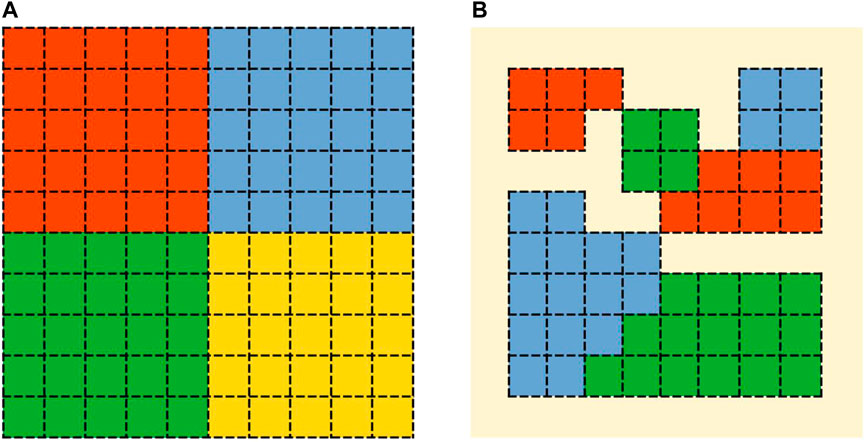
FIGURE 1. Model landscapes of (A) Parkhurst and Shogren (2007) with four agents (by colour) managing 25 land parcels each, and (B) the AgriPoliS parametrisation example in Brady et al. (2012) with three agents.
Some farmland models consider the spatial structure of landholdings in a more realistic manner. An example is the AgriPoliS model by Happe et al. (2008), which, since its development, has been used in numerous applied modelling studies throughout Europe (e.g., Happe et al., 2008; Brady et al., 2012; Hristov et al., 2020). A typical agricultural model landscape, as considered in AgriPoliS, was presented by Brady et al. (2012) and is reproduced in Figure 1B. It mimics typical farm structures, such as those shown in Figure 3 of Marie et al. (2009) and in Figure 3 of Pauchard et al. (2018).
Why is the spatial structure of the landholdings relevant? Agents under an AB are situated in a coordination game (van Huyck et al., 1990; Heinemann et al., 2004; Parkhurst and Shogren, 2007) in which a player’s reward is maximised if all players coordinate by spatially agglomerating their conservation efforts. Compared to that, the reward is somewhat reduced if the player does not coordinate (by conserving isolated low-cost land parcels); but it is minimised if they coordinate but the others do not. Both the coordinated and the uncoordinated states are Nash equilibria, and the establishment of the coordinated one is greatly enhanced if the agents can communicate (Parkhurst and Shogren, 2007; Banerjee et al., 2014; Banerjee et al., 2017). Thus, and quite obviously, the coordination problem would disappear if there were only a single agent who chooses the land-use pattern that maximises the total reward. On the opposite end, one can expect that the coordinated state is most difficult to establish if there are many agents, each of them owning only a single land parcel, as assumed in those studies mentioned above.
It is not clear how the spatial structure of landholdings affects the performance of the AB (and that of coordination in general) and whether and by how much the existing studies over- or underestimate the ability of landowners to coordinate their conservation efforts. To shed some light on these issues, this study considers a range of randomly created, stylised spatial landholding structures and evaluates them using a simple spatial land-use simulation model. The sampled model landscapes range from the case in which each landowner owns only a single land parcel, via landscapes similar to that shown in Figure 1B, to landscapes similar to that in Figure 1A.
For each sampled landscape, here, the model agents are subjected to an AB and the dynamics of their induced land use are stimulated. As functions of the regulator’s budget and the AB scheme design, this study determines the proportion and spatial agglomeration of conserved land parcels, as well as their ecological benefit (and hence, cost-effectiveness), assuming the conservation of a species with a limited dispersal range. The dependence of these scheme performance indicators on the described characteristics of the agents’ landholdings is analysed, as well as their dependence on other features, including the spatial variation and autocorrelation of the conservation costs and the species’ dispersal range.
In the next section, the rationale of the analysis is presented, as well as the structure and analysis of the model; followed by the presentation of the results and their discussion and a short concluding section.
2 Methods
2.1 Rationale
To demonstrate the (in fact, rather simple) reason why the size and spatial distribution of properties affect the performance of the agglomeration bonus, consider a square of four land parcels i = 1, … , 4, each owned by a single landowner. Each land parcel i can be conserved (xi = 1) or used for economic purposes (xi = 0). Conservation incurs a profit loss, henceforth termed conservation cost, ci. Table 1 shows a numerical example.

TABLE 1. Conservation costs of four land parcels arranged in a square.
Assume a conservation agency offers a base payment p = 55 for each conserved land parcel, plus a bonus b = 25 if the conserved land parcel is adjacent to another conserved land parcel (considering the eight movement directions of a chess king). I consider a sequence of contract periods—as, e.g., in the experiments by Parkhurst and Shogren (2007) or Banerjee et al. (2014), Banerjee et al. (2017). In each period, each landowner i myopically and independently chooses the profit-maximising land use xi that depends on the land uses of the other three land parcels j, k, and l and is given by
Assume all land parcels are initially used economically. Then, the base payment p = 55 > 50 induces conservation of the upper left land parcel of Table 1. In the second contract period, the other land parcels have one conserved neighbour each, so conservation of their land parcel would not only earn p = 55 but p + b = 80. However, this payment still falls short of the costs of all the other three land parcels, which stay in economic use altogether, only the upper left land parcel is conserved.
Now assume, alternatively, that there are only two landowners, where the first one owns the two left land parcels and the second one owns the two right land parcels. In the first contract period, each of the two landowners independently assesses four land-use strategies: all in economic use, conservation only of the upper land parcel, conservation only of the lower land parcel, and conservation of both land parcels. For the left landowner, the corresponding profits are 0, p – 50 = 5, p – 100 = –45, and 2p + 2b – 150 = 30. So, the most profitable decision is to conserve both land parcels. For the right landowner, the profits are 0, p – 100 = –45, p – 90 = –35, and 2p + 2b – 190 = –10, in that order, so the landowner uses both land parcels economically.
In the second contract period, the right landowner observes both the left land parcels to be conserved. Assuming constant conservation costs and a rational neighbouring landowner, they can be certain that these two land parcels will also be conserved in the second contract period. So, the profits of the four land-use strategies of the right landowner are now 0, p + 2b – 100 = 5, p + 2b – 90 = 15, and 2p + 6b – 190 = 70, rendering the conservation of both right land parcels profitable, so that in the second contract period, all four land parcels are conserved.
The difference between the two cases, four versus two landowners, is that in the latter case, each landowner can reap some of the agglomeration benefits (b) for themselves, and transfer surpluses (payment minus cost) from the least costly land parcel(s) to the more costly land parcel(s). So, conservation of the more costly land parcels becomes profitable, too. This effect is very similar to the surplus transfer effect coined by Drechsler et al. (2010), which is achieved by side payments between landowners.
Quite obviously, a major assumption for the existence of this difference between the two cases is that the landowners do not communicate with each other and make the land-use decisions independently and myopically. Otherwise, they could identify the coordinated state with all land parcels conserved right away. The simulation model in the next section allows for a more comprehensive analysis of the influence of the number and spatial distribution of the land parcels per landowner on the performance of the agglomeration bonus.
2.2 The model
Here, we consider two square grid landscapes of different sizes, one with N = 6 × 6 and one with N = 8 × 8 grid cells, each grid cell representing a land parcel. Conservation of a land parcel i ∈ {1, … , N} incurs a cost ci. The ci vary randomly among land parcels, normally distributed with mean one and standard deviation σ. The costs may be autocorrelated with spatial correlation length l [so that “cost hills” and “cost valleys” have spatial extents of about l; a numerical example and the description of the cost sampling method can be found in Drechsler et al. (2022)].
In the next step, the N land parcels are allocated to M agents by randomly selecting for each agent a central land parcel (“farmhouse”) and assigning the other land parcels randomly to one of the agents. The probability of a land parcel assigned to a particular agent exponentially declines with increasing distance to the central land parcel (Supplementary Appendix A). The rate of decline, α, is termed, henceforth, the “landholding cohesion parameter.”
A numerical example is shown in Figure 2. For α = 0 (panel a) the spatial distribution of the land ownership is completely random. The number of clusters with land parcels belonging to the same agent is 13, considering land parcels connected via joint edges or joint corners as neighbours. For α = 1 (panel b), the land parcels of landowner 3 tend to be in the upper left, those of landowner 2 in the lower left, those of landowner 4 in the upper right, and those of landowner 1 are dispersed. The number of clusters is 9. For α = 2 (panel c), the land parcels form 4 clusters and are clearly separated with crisp boundaries between them.
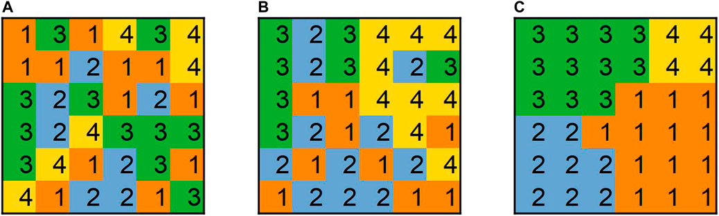
FIGURE 2. Spatial distribution of the landholdings of four landowners (numbered 1–4) in a model landscape with six-by-six land parcels. The property cohesion parameter is (from left to right) α = 0, 1, 2.
Each land parcel i in the so-defined landscape can be conserved (xi = 1) or used for economic purposes like intensive agriculture (xi = 0). Conservation is incentivised by an agglomeration bonus (AB), with spatially homogenous base payment p and a bonus b that is paid for each conserved neighbour within the 8-cell neighbourhood Ji around the focal (conserved) land parcel i:
Starting from an initially economically used landscape with all xi = 0, the agents determine the profits
of all their possible land-use strategies. These profits are the sum of the net revenues pi–ci of the conserved land parcels. Function δ(Oi, m) here is the “Kronecker-delta” that equals 1 if Oi = m and zero otherwise–to indicate whether land parcel i is owned by agent m or not.
As Eq. 2 indicates, the net revenue of a conserved land parcel i depends on the land uses in the neighbouring land parcels (which may belong to other landowners). Given the binary choice of choosing xi = 1 or xi = 0, an agent owning n land parcels evaluates and chooses between 2n different strategies (which are technically screened here via a recursive function). Each agent here assumes the (neighbours’) land use from the previous round (which, in the initial round, is xi = 0 for all i, as mentioned above). The agents do not communicate with each other, and land-use change is instantaneous, so an agent’s current decision is independent of the other agents’ current decisions.
The outcome of this analysis is a changed land-use pattern in which some of the xi may have turned to one. This new land-use pattern is the starting point for the next contract period, which is treated in the same way as described above, except that some of the xi may have changed to one. In the second period, some more of the previously zero-valued xi may change to one (the opposite change is impossible under the present model assumptions) and a new land-use pattern emerges. The simulation is continued until a maximum of ten contract periods is reached. In this way, the analysis is quite similar to the lab experiment of Parkhurst and Shogren (2007).
After the final (10th) period, the proportion of conserved land parcels
and their spatial aggregation, measured by the expected proportion γ of conserved land parcels around conserved land parcels,
are calculated. Next, the ecological benefit is calculated (Drechsler et al., 2010; Bareille et al., 2023)
which sums over all pairs of conserved land parcels, inversely weighted by their pairwise distance dij. It increases with increasing number and spatial aggregation of conserved land parcels. Parameter β may be regarded as the inverse of the mean dispersal distance of a species. An increasing β, i.e., decreasing species dispersal range, increases the importance of spatial aggregation.
Lastly, the regulator’s expenses are calculated by
2.3 Model analysis
To account for the randomness in the conservation costs and the land parcel ownerships, the analysis described in Section 2.2 is replicated several times and an average is taken for the four introduced performance indicators q, γ, V, and E. As a compromise between sampling error and computation time, the number of replicates is chosen: 500 for the small landscape with N = 36 and 200 for the large landscape with N = 64.
Being interested, among other things, in the cost-effectiveness of the AB, where the ecological benefit V is maximised for the given conservation budget B, a number of discrete budget levels B are defined (see below). Since the regulator’s expenses E increase both with increasing base payment p and bonus b, there is an infinite number of combinations (p, b) that lead to the full exhaustion of the budget B. To find the budget-exhausting level of p for the given bonus b (for the considered levels of b, see below) the base payment p is varied to match E with B. The minimisation of the deviation between E and B is carried out via Newton’s secant method (allowing for a relative error, |E/B–1|, of up to 5%).
Five levels for the budget B are considered, defined by the amounts that would be required to conserve 2.5, 7, 16, 31, and 50% of the land parcels under a homogenous payment p (with bonus b = 0). These bounds well encompass the range of typical enrolment rates for agri-environment schemes in EU countries (Tyllianakis and Martin-Ortega, 2021). In Supplementary Appendix B, the five associated levels for the base payment p (Table 2) as well as three values for the bonus b are derived (Table 3).
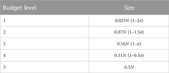
TABLE 2. The five considered budget levels.
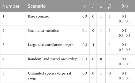
TABLE 3. Values of the model parameters conservation cost variation σ, conservation cost correlation length l, landholding cohesion parameter α, inverse species dispersal range β, and bonus b.
The number of agents M is varied from 3 to 36 for the small landscape N = 36 and from 7 to 64 for the larger landscape N = 64. The upper values of 36 and 64, respectively, represent the cases in which each agent owns one single land parcel. The lower bounds on M are critically determined by computation time, which exponentially increases with the increasing number of land parcels per landowner. Altogether, the analysis yields for each budget level and each level of M the mean values (with the means taken over the randomly sampled model landscapes) of the three scheme performance indicators q, γ, and V.
The above parameter sweeps are performed for five model parameter combinations (“scenarios”) and three levels of the bonus b. The scenarios are formed by setting all model parameters at some base values (scenario 1) and from there, varying each parameter individually to another value. To choose the base values, the number of agents M (or equivalently, the number of land parcels owned by each agent: ∼N/M) is hypothesised to have a particularly strong influence on the performance indicators of the AB if
• The cost variation σ is large,
• The correlation length l of the costs is small (because here, a homogenous payment would lead to a completely random pattern of conserved land parcels and the AB is most important to induce spatial aggregation: see, e.g., Drechsler et al. (2010),
• The properties of the different agents are spatially cohesive and have distinct boundaries with the other agents’ properties, which is achieved by a high landholding cohesion parameter α (Figure 2), and
• The species has a small dispersal range, i.e., the inverse dispersal distance β is large.
From these values that define the base scenario in Table 2, the model parameters are varied to alternative values at which the impact of M is expected to be smaller, i.e., smaller σ, larger l, zero α, and zero β (Table 3). A justification of the chosen values of σ, l, α, and β is provided in Supplementary Appendix B.
To assess the relative influence of landowner number M on the performance variables q, γ, and V (for the given budget) for a particular scenario, we take the mean m1 of the considered performance variable (for the given budget level, Table 1) over the three smallest levels of M (3, 4, 5 for N = 36, and 7, 8, 9 for N = 64) and the mean m2 over the three largest levels of M (30, 31, 32 for N = 36 and 62, 63, 64) for N = 64 (this averaging is to smooth out the randomness in the model results) and calculate the ratio
3 Results
The results are presented in three steps. First, to explore the influence of the number of agents, M, on the performance of the AB, the three performance indicators q, γ, and V (Eqs 4–6 are shown as functions of M, for the five budget levels of Table 2 in the base scenario of Table 3. Second, to understand the influences of the model parameters σ, l, α, and β (cf. Table 3), the ratio r of Eq. 8 that measures the impact of M on the scheme performance is shown for each of the five scenarios defined in Table 3. Lastly, to assess the influence of the bonus b, the scheme cost-effectiveness (V) is shown, for the base scenario, as a function of M, for the three levels of b (Table 3) and three budget levels.
Figure 3 shows that the three AB performance indicators (proportion q and agglomeration γ of conserved land parcels, and ecological benefit V (cost-effectiveness)) decrease with the increasing number of agents M (i.e., decreasing number of land parcels per landowner). As expected, they increase with increasing budget. The largest influences of M are generally observed for larger budgets, with the ratios r between the outcomes for small and large M reaching values around 0.25.
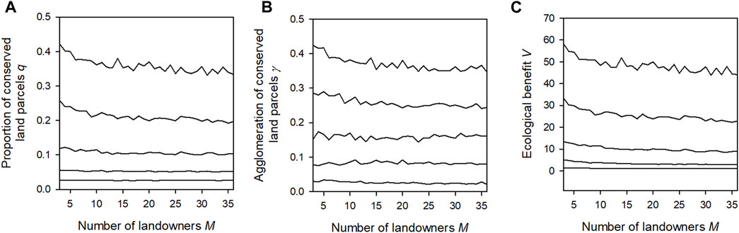
FIGURE 3. Proportion q and spatial agglomeration γ of conserved land parcels (A,B) and ecological benefit V (C) as functions of the number of model agents M, for a given conservation budget (B). Shown for the five budget levels of Table 2 (lines increasing from bottom to top). Model parameters as defined for the base scenario of Table 3, with a large bonus of b = 0.5σ. The number of land parcels is N = 6 × 6 = 36.
The effects of the model parameters (scenarios) on these effects of M are less clear than hypothesised (Figure 4). A low-cost variation (Figure 4, scenario 2) does reduce the effect of M on the proportion q and the benefit V (Figures 4A, C), but the effect of M on the spatial agglomeration γ seems to be quite independent of the cost variation and of all model parameters altogether (Figure 4B). A positive cost correlation length (scenario 3) slightly reduces the effect of M on q and γ and considerably reduces its effect on V.
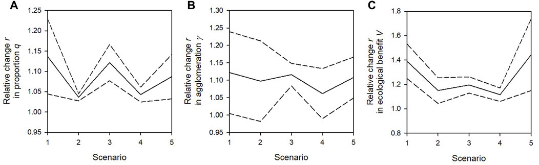
FIGURE 4. Relative influence r (Eq. 8) of the number of landowners M on the proportion and spatial agglomeration γ of conserved land parcels (A,B) and the ecological benefit V (cost-effectiveness, (C) for five different scenarios. Since the dependence of r on the budget B differs between scenarios (and no unique pattern can be detected such that r always increases or decreases with increasing B) the mean (solid line) and the “range” (mean plus/minus one standard deviation: dashed lines) of r over the five budget levels is shown.
As hypothesised, if the land parcels are not cohesive per landowner but the landholdings are strongly fragmented (α = 0), the influence of M is weakened for all three performance indicators (scenario 4). Other than hypothesised, an unlimited dispersal range (β = 0, scenario 5) increases the influence of M on the ecological benefit V. The reason is that for β = 0, we have V(β = 0) = q2, so the spatial agglomeration of conserved land parcels has no influence on the benefit function V, which instead quadratically increases with increasing q. Thus, the influence of M on q (i.e., decreasing M increases q, Figure 3A) is amplified in V.
The final issue of interest is the cost-effective level of the bonus b. Since only three levels of b were considered, it is determined which of these three levels generates, for the given budget, the highest ecological benefit V. Figure 5 delivers three insights. First, with increasing budget, smaller levels of the bonus become cost-effective. The reason is that there is a trivial correlation between the proportion q and the spatial agglomeration γ of conserved land parcels in the sense that, necessarily, γ ≥ q. So, even for a zero bonus, a high budget implies, via a high q, a high γ. Consequently, smaller bonuses are required to achieve the cost-effective level of spatial agglomeration.
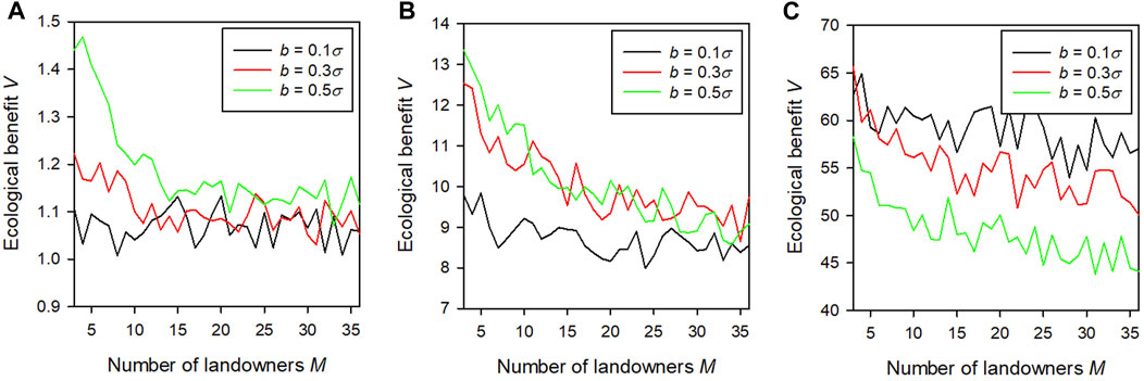
FIGURE 5. Ecological benefit V (level of cost-effectiveness) as a function of the number of landowners M. The colours represent the bonus level b. (A–C) show, from left to right, the results for the smallest, medium, and largest budgets, i.e., levels 1, 3, and 5 of Table 2. The model parameters σ, l, α, and β are set at their baseline values (Scenario 1 in Table 3).
Second, the effect of the landowner number M is higher for larger bonus levels. This implies that, third, the relative advantage of a given bonus level relative to other levels changes with changing M. In particular, for the smallest budget (Figure 5A), at large M, the largest bonus b = 0.5σ is only slightly more cost-effective than the other two bonus levels, while at small M, it is much more cost-effective. A similar result is observed for the medium budget (Figure 5B), where there is even a small rank reversal: while for large M, the largest bonus level appears slightly less cost-effective than the medium level (b = 0.3σ), at small M, it is clearly more cost-effective.
For the largest budget (Figure 5C), at large M, the smallest bonus level (b = 0.1σ) is clearly more cost-effective than the other two levels, while at small M, it is about as cost-effective as the medium bonus level. The results of N = 64 land parcels Figs. C1–3 of Supplementary Appendix C are very similar to those presented in Figure 5.
4 Discussion
Coordination incentives like the agglomeration bonus of Parkhurst et al. (2002) in which conservation of a land parcel earns a base payment, plus an additional bonus if that land parcel is adjacent to other conserved land parcels, have been proposed to induce the spatial agglomeration of conservation efforts. Many of the numerical and simulation studies, as well as experimental studies, that have contributed to a better understanding of the functioning of the AB assume that each landowner owns only a single land parcel that can either be conserved or used for economic purposes like intensive agriculture. On the opposite end of the spectrum, other studies assume that landowners own several land parcels, but these land parcels are arranged in cohesive blocks, with crisp boundaries between the properties of different landowners.
Both assumptions are not realistic. Instead, real landholdings are fragmented (Marie et al., 2009; LaTruffe and Piet, 2014; Pauchard et al., 2018). The present simulation analysis reveals that the number of land parcels per landowner and their spatial distribution matters. A decreasing number of landowners (so that each landowner owns an increasing number of land parcels), and a declining level of fragmentation of the landholdings (so that the landholdings become spatially cohesive as, e.g., in Figure 2C; rather than fragmented as, e.g., in Figure 2A) increase the proportion and spatial agglomeration of land parcels as well as the cost-effectiveness (ecological benefit for given conservation budget) of the scheme.
The reason for this finding is that adjacent land parcels allow the landowner to transfer the economic surpluses from agglomeration from high-cost to low-cost land parcels (as outlined in Section 2.1); so, for the given base payment and bonus, they will conserve more land. While, if the land parcels of each landowner are dispersed and surrounded by the land parcels of other landowners, the situation is similar to that in which each landowner owns only a single land parcel, and where surpluses are not transferred and coordination of conservation efforts is impeded.
These observed effects are especially large if 1) the conservation costs are spatially heterogeneous and spatially uncorrelated and 2) the bonus is large. To avoid a misunderstanding about the latter result, it should be noted that all the analyses are carried out under a fixed conservation budget so that a larger bonus is accompanied by a smaller base payment in order to meet the budget constraint.
The reason for result 1) is that the AB is meant to offset the cost difference between less costly but isolated land parcels and connected but costly land parcels (e.g., Parkhurst and Shogren, 2007; Drechsler et al., 2010); so, it is most effective if there is sufficient variation in the costs of neighbouring land parcels. Result 2) is obtained because the above-described internal surplus transfer from low-cost to high-cost land parcels within each landholding is most effective and relevant if the bonus is large.
Result 2) implies that the number of land parcels per landowner affects the cost-effective level of the bonus. The analysis reveals that with an increasing number of land parcels per landowner, larger bonus levels (and accordingly smaller base payments) become more cost-effective relative to smaller ones (which, of course, does not mean larger bonus levels are always more cost-effective than smaller levels, since this depends on many other ecological and economic parameters). The reason is, again, that the described “internal surplus transfer” is most effective when the landholdings are spatially cohesive.
As the rationale of Section 2.1 reveals, the results are driven by the assumption that the landowners do not communicate with each other, which would allow for transferring agglomeration surpluses between landowners, as in Drechsler et al. (2010), and more conservation and agglomeration could be achieved for given levels of base payment and bonus. The landowners also do not decide strategically, which implies that they are locked in the uncoordinated Nash equilibrium (cf. Parkhurst and Shogren, 2007) and that they can leave only with sufficiently high levels of the bonus. With strategic behaviour (Drechsler, 2023) and communication (Parkhurst and Shogren, 2007; Banerjee et al., 2014; Banerjee et al., 2017), in contrast, the coordinated Nash equilibrium could be found more easily.
Future research may explore the role of strategic behaviour and communication between landowners in more detail. Further issues of interest would be different types of coordination incentives, like threshold payments (Nguyen et al., 2022). Like most theoretical and experimental studies of coordination incentives, the present analysis is based on a number of simplifying assumptions, e.g., about the landowner behaviour, the consideration of only two land-use types, and the structure of the model landscapes. These abstract landscapes ignore many details of real landscapes to focus on the spatial structure of the landholdings and to allow for a systematic variation between large and small landholdings and between cohesive and fragmented landholdings. An application of the model to a real agricultural landscape, therefore, would be a fruitful avenue for future research.
5 Conclusion
The analysis highlights the substantial influence of the spatial structure of landholdings on the dynamics and performance of coordination incentives, represented here by the agglomeration bonus (AB). The smaller and the more fragmented the landholdings are, the more difficult is it for landowners to coordinate their conservation efforts and the lower the cost-effectiveness of the AB, especially if the conservation costs vary strongly in space. As a consequence, the cost-effective scheme design, too, depends on the spatial structures of the landholdings. Especially when the landholdings are spatially dispersed, the facilitation of communication between landowners is an important instrument for the enhancement of coordination and scheme performance.
Data availability statement
The original contributions presented in the study are included in the article/Supplementary Material, further inquiries can be directed to the corresponding author.
Author contributions
MD: Writing–original draft, Writing–review and editing.
Funding
The author(s) declare that no financial support was received for the research, authorship, and/or publication of this article.
Conflict of interest
The author declares that the research was conducted in the absence of any commercial or financial relationships that could be construed as a potential conflict of interest.
The author(s) declared that they were an editorial board member of Frontiers, at the time of submission. This had no impact on the peer review process and the final decision.
Publisher’s note
All claims expressed in this article are solely those of the authors and do not necessarily represent those of their affiliated organizations, or those of the publisher, the editors and the reviewers. Any product that may be evaluated in this article, or claim that may be made by its manufacturer, is not guaranteed or endorsed by the publisher.
Supplementary material
The Supplementary Material for this article can be found online at: https://www.frontiersin.org/articles/10.3389/fenvs.2023.1233758/full#supplementary-material
References
Albers, H. J., Ando, A. W., and Batz, M. (2008). Patterns of multi-agent land conservation: crowding in/out, agglomeration, and policy. Resour. Energy Econ. 30 (4), 492–508. doi:10.1016/j.reseneeco.2008.04.001
Arora, G., Feng, H., Hennessy, D. A., Loesch, C. R., and Kvas, S. (2021). The impact of production network economies on spatially-contiguous conservation – theoretical model with evidence from the U.S. Prairie Pothole Region. J. Environ. Econ. Manag. 107, 102442. doi:10.1016/j.jeem.2021.102442
Banerjee, S., Cason, T. N., de Vries, F. P., and Hanley, N. (2017). Transaction costs, communication and spatial coordination in Payment for Ecosystem Services schemes. J. Environ. Econ. Manag. 87, 68–89. doi:10.1016/j.jeem.2016.12.005
Banerjee, S., de Vries, F. P., Hanley, N., and van Soest, D. P. (2014). The impact of information provision on agglomeration bonus performance: an experimental study on local networks. Am. J. Agric. Econ. 96, 1009–1029. doi:10.1093/ajae/aau048
Banerjee, S., Kwasnica, A. M., and Shortle, J. S. (2012). Agglomeration bonus in small and large local networks: a laboratory examination of spatial coordination. Ecol. Econ. 84, 142–152. doi:10.1016/j.ecolecon.2012.09.005
Bareille, F., Zavalloni, M., and Viaggi, D. (2023). Agglomeration bonus and endogenous group formation. Am. J. Agric. Econ. 105, 76–98. doi:10.1111/ajae.12305
Bell, A. R., Parkhurst, G., Droppelmann, K., and Benton, T. G. (2016). Scaling up pro-environmental agricultural practice using agglomeration payments: proof of concept from an agent-based model. Ecol. Econ. 126, 32–41. doi:10.1016/j.ecolecon.2016.03.002
Bell, A. R., Ward, P. S., Mapemba, L., Nyirenda, Z., Msukwa, W., and Kenamu, E. (2018). Smart subsidies for catchment conservation in Malawi. Sci. Data 5, 180113. doi:10.1038/sdata.2018.113
Brady, M., Sahrbacher, C., Kellermann, K., and Happe, K. (2012). An agent-based approach to modeling impacts of agricultural policy on land use, biodiversity and ecosystem services. Landsc. Ecol. 27, 1363–1381. doi:10.1007/s10980-012-9787-3
Delacote, P., Robinson, E. J., and Roussel, S. (2016). Deforestation, leakage and avoided deforestation policies: a spatial analysis. Resour. Energy Econ. 45, 192–210. doi:10.1016/j.reseneeco.2016.06.006
Dijk, J., Ansink, E., and van Soest, D. (2017). Buyouts and agglomeration bonuses in wildlife corridor auctions. Tinbergen Inst. Discuss. Pap. doi:10.2139/ssrn.2946850
Drechsler, M. (2023). Improving models of coordination incentives for biodiversity conservation by fitting a multi-agent simulation model to a lab experiment. J. Behav. Econ. Exp. 102, 101967. doi:10.1016/j.socec.2022.101967
Drechsler, M., Johst, K., Wätzold, F., and Shogren, J. F. (2010). An agglomeration payment for cost-effective biodiversity conservation in spatially structured landscapes. Resour. Energy Econ. 32, 261–275. doi:10.1016/j.reseneeco.2009.11.015
Drechsler, M., Wätzold, F., and Grimm, V. (2022). The hitchhiker's guide to generic ecological-economic modelling of land-use-based biodiversity conservation policies. Ecol. Model. 465, 109861. doi:10.1016/j.ecolmodel.2021.109861
Happe, K., Balmann, A., Kellermann, K., and Sahrbacher, C. (2008). Does structure matter? The impact of switching the agricultural policy regime on farm structures. J. Econ. Behav. Organ. 67, 431–444. doi:10.1016/j.jebo.2006.10.009
Heinemann, F., Nagel, R., and Ockenfels, P. (2004). Measuring strategic uncertainty in coordination games. Munich: Center for Economic Studies and ifo Institute CESifo. CESifo Working Paper, No. 1364. Available at: https://www.econstor.eu/bitstream/10419/18727/1/cesifo1_wp1364.pdf (Accessed October 17, 2023).
Hristov, J., Clough, Y., Sahlin, U., Smith, H., Stjernman, M., Olsson, O., et al. (2020). Impacts of the EU's common agricultural policy “greening” reform on agricultural development, biodiversity, and ecosystem services. Appl. Econ. Perspect. Policy 42, 716–738. doi:10.1002/aepp.13037
Huber, R., Zabel, A., Schleiffer, M., Vroege, W., Brändle, J. M., and Finger, R. (2021). Conservation costs drive enrolment in agglomeration bonus scheme. Ecol. Econ. 186, 107064. doi:10.1016/j.ecolecon.2021.107064
Iftekhar, Md.S., and Tisdell, J. G. (2016). An agent based analysis of combinatorial bidding for spatially targeted multi-objective environmental programs. Environ. Resour. Econ. 64, 537–558. doi:10.1007/s10640-015-9882-4
Krämer, J. E., and Wätzold, F. (2018). The agglomeration bonus in practice – an exploratory assessment of the Swiss network bonus. J. Nat. Conservation 43, 126–135. doi:10.1016/j.jnc.2018.03.002
Krawczyk, M., Bartczak, A., Hanley, N., and Stenger, A. (2016). Buying spatially-coordinated ecosystem services: an experiment on the role of auction format and communication. Ecol. Econ. 124, 36–48. doi:10.1016/j.ecolecon.2016.01.012
Kuhfuss, L., Préget, R., Thoyer, S., de Vries, F. P., and Hanley, N. (2022). Enhancing spatial coordination in payment for ecosystem services schemes with non-pecuniary preferences. Ecol. Econ. 192, 107271. doi:10.1016/j.ecolecon.2021.107271
LaTruffe, L., and Piet, L. (2014). Does land fragmentation affect farm performance? A case study from Brittany, France. Agric. Syst. 129, 68–80. doi:10.1016/j.agsy.2014.05.005
Marie, M., Bensaid, A., and Delahaye, D. (2009). Le rôle de la distance dans l’organisation des pratiques et des paysages agricoles: l’exemple du fonctionnement des exploitations laitières dans l’arc atlantique. Cybergeo Eur. J. Geogr. doi:10.4000/cybergeo.22366
Nguyen, C., Latacz-Lohmann, U., Hanley, N., Schilizzi, S., and Iftekhar, S. (2022). Spatial Coordination Incentives for landscape-scale environmental management: a systematic review. Land Use Policy 114, 105936. doi:10.1016/j.landusepol.2021.105936
Panchalingam, T., Ritten, C. J., Shogren, J. F., Ehmke, M. D., Bastian, C. T., and Parkhurst, G. M. (2019). Adding realism to the Agglomeration Bonus: how endogenous land returns affect habitat fragmentation. Ecol. Econ. 164, 106371. doi:10.1016/j.ecolecon.2019.106371
Parkhurst, G. M., and Shogren, J. F. (2007). Spatial incentives to coordinate contiguous habitat. Ecol. Econ. 64, 344–355. doi:10.1016/j.ecolecon.2007.07.009
Parkhurst, G. M., Shogren, J. F., Bastian, C., Kivi, P., Donner, J., and Smith, R. B. W. (2002). Agglomeration bonus: an incentive mechanism to reunite fragmented habitat for biodiversity conservation. Ecol. Econ. 41, 305–328. doi:10.1016/S0921-8009(02)00036-8
Parkhurst, G. M., Shogren, J. F., and Crocker, T. (2016). Tradable set-aside requirements (TSARs): conserving spatially dependent environmental amenities. Environ. Resour. Econ. 63, 719–744. doi:10.1007/s10640-014-9826-4
Pauchard, L., Marie, M., and Madeline, P. (2018). “Les échanges parcellaires dans l’ouest français: du diagnostic à la proposition de groupes de travail,” in Infinite rural systems in a finite planet: bridging gaps towards sustainability. Editors V. P. Carril, R. C. L. González, J. N. T. Santamaría, and F. H. McKenzie (Santiago de Compostela, Spain: Universidade de Santiago de Compostela), 115–122. https://hal.science/hal-01913271/document.
Tyllianakis, E., and Martin-Ortega, J. (2021). Agri-environmental schemes for biodiversity and environmental protection: how we are not yet “hitting the right keys”. Land Use Policy 109, 105620. doi:10.1016/j.landusepol.2021.105620
van Huyck, J. B., Battalio, R. C., and Beil, R. O. (1990). Tacit coordination games, strategic uncertainty, and coordination failure. Am. Econ. Rev. 80, 234–248. Available at: http://www.jstor.org/stable/2006745 (Accessed October 17, 2023).
Keywords: agent-based model, agglomeration bonus, coordination incentives, cost-effectiveness, land fragmentation, spatial distribution
Citation: Drechsler M (2023) The influence of farmland distribution on the performance of the agglomeration bonus. Front. Environ. Sci. 11:1233758. doi: 10.3389/fenvs.2023.1233758
Received: 24 July 2023; Accepted: 30 October 2023;
Published: 05 December 2023.
Edited by:
Tolera Senbeto Jiren, International Center for Biosaline Agriculture (ICBA), United Arab EmiratesReviewed by:
Stuart Pimm, Duke University, United StatesSita Koné, International Center for Biosaline Agriculture (ICBA), United Arab Emirates
Copyright © 2023 Drechsler. This is an open-access article distributed under the terms of the Creative Commons Attribution License (CC BY). The use, distribution or reproduction in other forums is permitted, provided the original author(s) and the copyright owner(s) are credited and that the original publication in this journal is cited, in accordance with accepted academic practice. No use, distribution or reproduction is permitted which does not comply with these terms.
*Correspondence: Martin Drechsler, bWFydGluLmRyZWNoc2xlckB1ZnouZGU=