Dissolved oxygen concentration inversion based on Himawari-8 data and deep learning: a case study of lake Taihu

Dissolved Oxygen (DO) concentration is an essential water quality parameter widely used in water environments and pollution assessments, which indirectly reflects the pollution level and the occurrence of blue-green algae. With the advancement of satellite technology, the use of remote sensing techniques to estimate DO concentration has become a crucial means of water quality monitoring. In this study, we propose a novel model for DO concentration estimation in water bodies, termed Dissolved Oxygen Multimodal Deep Neural Network (DO-MDNN), which utilizes synchronous satellite remote sensing data for real-time DO concentration inversion. Using Lake Taihu as a case study, we validate the DO-MDNN model using Himawari-8 (H8) satellite imagery as input data and actual DO concentration in Lake Taihu as output data. The research results demonstrate that the DO-MDNN model exhibits high accuracy and stability in DO concentration inversion. For Lake Taihu, the performance metrics including adj_R², RMSE, Pbias, and SMAPE are 0.77, 0.66 mg/L, −0.44%, and 5.36%, respectively. Compared to the average performance of other machine learning models, the adj_R² shows an improvement of 6.40%, RMSE is reduced by 8.27%, and SMAPE is decreased by 12.1%. These findings highlight the operational feasibility of real-time DO concentration inversion using synchronous satellite data, providing a more efficient, economical, and accurate approach for real-time DO monitoring. This method holds significant practical value in enhancing the efficiency and precision of water environment monitoring.

1 Introduction

In recent years, the rapid growth of population, accelerated industrialization, and excessive use of fertilizers and pesticides have resulted in numerous adverse effects on the water quality of lakes. As a consequence, local lake environments are facing serious deterioration in water quality and eutrophication issues (e.g., Liu et al., 2019; Liang et al., 2021). Therefore, enhancing the capability of water quality monitoring and timely understanding the changes in lake water environments are of great significance for lake protection and pollution control (e.g., Lyu et al., 2015; Batur and Maktav, 2018; Chen et al., 2021). Dissolved Oxygen (DO) concentration is a commonly used water quality indicator in water environments and pollution studies. Monitoring the spatio-temporal variations of DO has become crucial in assessing water environments. DO, primarily originated from atmospheric diffusion, biological photosynthesis, and runoff, is influenced by factors such as radiation flux density, precipitation, and water nutrient concentrations. If the water body becomes eutrophic, it can lead to abnormal proliferation of cyanobacteria, and the decomposition of microorganisms and organic matter can significantly deplete DO concentrations (e.g., Ma et al., 2013). The decrease in DO concentration has various adverse effects on the ecological diversity of the region. It leads to the death of other organisms in the water and results in discoloration and foul odor (e.g., Guo et al., 2021). Therefore, DO concentration can indirectly describe the degree of water pollution and reflect the ecological and pollution status of the water body.

Traditional water quality monitoring methods rely on manual sampling or station monitoring, which can provide certain monitoring data (e.g., Zhang et al., 2022). However, these methods are costly for deploying monitoring buoys, and have a limited effective monitoring range, which makes it difficult to observe the dynamic changes of pollution on a macro scale (e.g., Sagan et al., 2020). With the continuous improvement in the spatial and temporal resolution of satellite remote sensing data, the use of satellite remote sensing data for water quality inversion has gradually become an important approach for monitoring surface water quality (e.g., Batur and Maktav, 2018). In current research, DO is primarily inferred indirectly through optically active constituents (OACs) or directly through remote sensing reflectance (Rrs). In terms of indirect inference using OACs, Guo et al. (2021) used Landsat and MODIS satellite data and employed a Support Vector Regression (SVR) model with strong generalization capability to estimate the measured DO concentration in four lakes. The study successfully reproduced the spatial distribution and monthly variation of DO in Lake Huron from 1984 to 2000. Peterson et al. (2020) utilized the relationship between OACs and NOACs to apply deep learning methods for anomaly detection of DO. Their approach successfully identified water quality anomalies. Kim et al. (2020) established a multiple regression analysis model based on the correlation between DO, water temperature, and Chlorophyll-a (Chl-a), demonstrating the potential monitoring capability of satellite remote sensing in high spatio-temporal resolution DO concentration. Regarding direct estimation using Rrs, Karakaya and Evrendilek. (2011) proposed a simple approach based on optimal fit multiple linear regression to estimate DO concentrations using Landsat 7 data. Sharaf, et al. (2017) developed a backpropagation neural network to estimate DO using Landsat 8 data and mapped the spatial distribution of DO concentrations in the Saint John River in Canada. Batur and Maktav. (2018) estimated DO concentrations in Lake Gala (Turkey) using data fusion and mining techniques, such as principal component analysis (PCA), with the assistance of Landsat 8 and Sentinel-2A. These studies demonstrate the potential of remote sensing satellites in monitoring DO concentrations at high spatial and temporal resolutions. For learning features from a single modal (such as text, audio, or video), Artificial Neural Network (ANN) is the most direct learning approach in general. However, different modalities exhibit a complementary yet imbalanced relationship. Inspired by the way humans perceive and process complex information through multiple senses (e.g., vision, hearing), Ngiam, et al. (2018) from Stanford University proposed Multimodal Deep Learning (MDL). In contrast to a single modal, one of the ideas behind multimodal learning is to employ multiple independent sub neural networks (sNNs) to learn features from different modalities. The learned results are then fused and inputted into a new sNN for prediction, enabling the fusion of information from various modalities and facilitating the exchange of information between them. During the training process, a single modal often fails to encompass all the necessary information for producing accurate outputs. By incorporating information from multiple modalities, the multimodal network training process achieves information supplementation, expands the coverage of information contained in the input data, enhances model accuracy, and improves model robustness.

However, previous studies often used polar-orbiting remote sensing satellites, which have low revisit rates for the same location (e.g., Sentinel-2 (e.g., Peterson et al., 2020; Wang et al., 2022) with a revisit period of 5 days, and Landsat-8 (e.g., Chen and Quan, 2012) with even longer intervals of 16 days), often requiring several years of data accumulation to establish effective inversion models.

The new generation geostationary satellite, Himawari-8 (H8) possesses high temporal resolution (e.g., Wang et al., 2017; Wang et al., 2020; Ning et al., 2021). Compared to commonly used polar-orbiting satellites for water quality remote sensing, it offers a higher revisit rate, which allows for repeated sampling of the same location every 10 min. This makes it suitable for monitoring continuous changes in water quality and provides important data support for environmental monitoring. Some researchers have already conducted effective monitoring studies using H8 satellite remote sensing data. Wang et al. (2017) utilized H8 satellite remote sensing data for dynamic monitoring of cyanobacterial blooms in lake Taihu. Chen. (2019), with the support of H8 satellite remote sensing data, effectively monitored floating algae, achieved better monitoring results than the Geostationary Ocean Color Imager (GOCI) satellite (with a revisit period of 1 h). These research findings demonstrate that the high revisit rate characteristic of the H8 satellite can capture more frequent water quality changes, thereby detecting phenomena that may be missed by existing satellites (such as the GOCI satellite) and providing robust data support for the continuous and dynamic monitoring of lake water quality (e.g., Yang et al., 2021). Currently, there is no existing research on DO concentration inversion using H8 satellite remote sensing data. This study aims to establish a correlation model between H8 satellite remote sensing data and DO concentration through machine learning or deep learning algorithms to achieve real-time monitoring of DO concentration.

This study takes Lake Taihu as an example to construct a high-precision deep learning model based on H8 satellite remote sensing data for estimating DO concentration. The main objective is to provide an efficient inversion method for monitoring DO indicators in Lake Taihu and other inland lakes, aiming to reduce monitoring time delays and improve inversion accuracy. This research plays a crucial role in strengthening the management of organic pollution in lakes, supporting water environment pollution prevention and control, pollutant source tracing, and water quality monitoring and early warning. It is expected to serve as a valuable supplement to water quality remote sensing inversion and estimation methods.

2 Materials and methods

2.1 Research area overview

Lake Taihu, as shown in Figure 1, is the third largest freshwater lake in China. It is located in the southern part of Jiangsu Province, between 119°52′32″E to 120°36′10″E and 30°55′40″N to 31°32′58″N. The lake is situated in the economic core area of the Yangtze River Delta and provides daily water supply for irrigation, domestic use, transportation, and other purposes for the surrounding residents. Lake Taihu has a surface area of 2,427.8 km², a water area of 2,338.11 km², a shoreline length of 393.2 km, an average depth of 1.9 m, a maximum depth of 2.6 m, and a total storage capacity of approximately 5 billion m³ (e.g., Lyu et al., 2015).

FIGURE 1

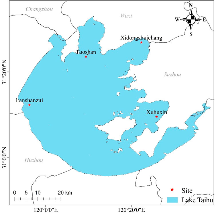
FIGURE 1. Map of Lake Taihu’s Scope and Distribution of Monitoring Sections.

The surrounding areas of lake Taihu suffer from significant pollution, frequent algal blooms, and widespread accumulation of cyanobacteria, which keep the lake in a state of mild eutrophication (e.g., Ma et al., 2008; Zhang et al., 2010; Zhu et al., 2021). The Ecological Environment Reports of Wuxi City, Suzhou City, and Changzhou City in 2021 (e.g., Changzhou Ecological Environment Bureau, 2021; Suzhou Ecological Environment Bureau, 2021; Wuxi Ecological Environment Bureau, 2021) indicated that, according to the “Surface Water Environmental Quality Standards” (GB3838-2002), the overall water quality of lake Taihu during the year was classified as Class IV. The comprehensive nutrient status index ranged from 53.3 to 59.5, indicating a mild eutrophication status.

2.2 Data and preprocessing

2.2.1 DO data

The DO measured data used in this study were obtained from the Comprehensive Business Portal of the Ministry of Ecology and Environment, which provides real-time data from the national automatic monitoring system for surface water quality during the “13th Five-Year Plan” period. The selected data includes DO (mg/L) and water temperature (°C) indicators from four monitoring sections within the Lake Taihu Basin, covering the period from January 1, 2019, to December 31, 2021 (Table 1). The data collection frequency is 1 h per measurement, and it adheres to the technical specifications for automatic monitoring of surface water (HJ 915-2017).

TABLE 1

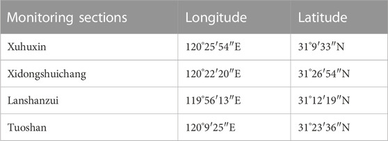
TABLE 1. Latitude and Longitude information of monitoring sections in lake Taihu.

Due to the potential influence of environmental changes or instrument malfunctions during data collection at water quality automatic monitoring stations, it is necessary to address missing and abnormal data to ensure the accuracy of data used for model fitting. Missing values in the obtained DO data were excluded, and the 3σ principle was applied. Concentration data falling within the range of $\left.{\left[DO\right.}_{mean}-3\times {DO}_{std},{DO}_{mean}-3\times {DO}_{std}\right]$ were retained as the measured DO data for the model, while data outside this range were considered abnormal and removed. Here, ${DO}_{mean}$ represents the average DO concentration for the current monitoring section, and ${DO}_{std}$ is the standard deviation of DO concentration for the same section.

2.2.2 Synchronous satellite data

H8 satellite carries an advanced optical sensor, namely, Advanced Himawari Imager (AHI), which includes 3 visible light bands, 3 near-infrared bands, and 10 infrared bands. It captures full-disc images of the Earth every 10 min. These images provide high-frequency coverage of the entire Asia-Pacific region, which includes Asia, Oceania, and part of the Pacific Ocean. The specific coverage area is approximately half of the Earth, equivalent to about 3.9 million square miles. It possesses characteristics of high spatial coverage and high temporal resolution. The H8 satellite remote sensing data used in this study is obtained from the Himawari Monitoring System P-free (https://www.eorc.jaxa.jp/ptree/), accessed on 15 July 2022, which provides full-disc satellite images with a spatial resolution of 2 km. Data from the H8 satellite were selected from January 1, 2019, to December 31, 2021, with hourly sampling to match the temporal resolution of the DO measured data. In total, 26258 images were acquired. Channels 1 to 16 were used for DO inversion, where channels 1–6 were mainly used to obtain visible light and infrared images for monitoring cloud cover, atmospheric details, and temperature, as well as studying weather patterns and cloud formation; Channels 7–16 were primarily used for infrared temperature detection and high-resolution infrared images to detect atmospheric temperature, water vapor distribution, cloud characteristics and properties, as well as observe cloud and surface temperature distribution. The H8 satellite data used are L1-level data, the data file format is Network Common Data Form (NetCDF), the spatial resolution is 2 km × 2 km, the temporal resolution is 10 min/times, and the wavelength ranges and uses of each channel of data are shown in the Table 2.

TABLE 2

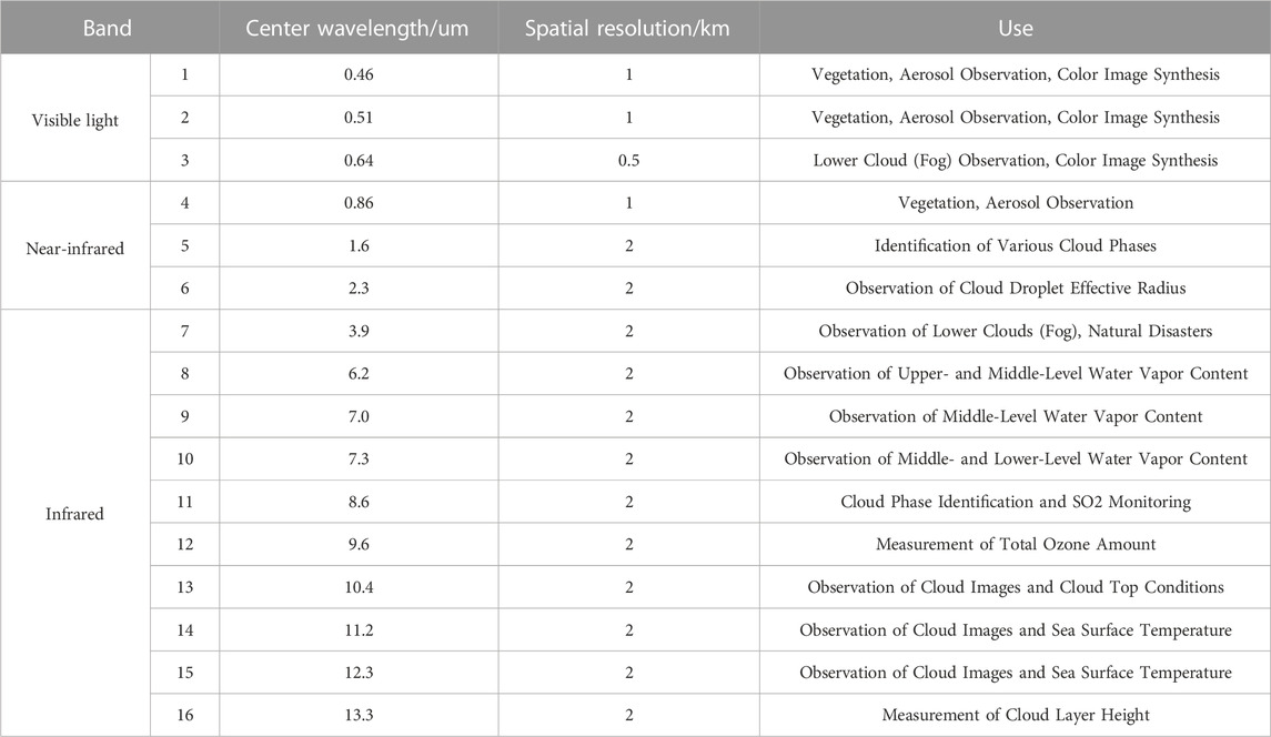
TABLE 2. Information parameters by band.

The H8 satellite has unique advantages over other satellites in lake water quality monitoring. Firstly, H8 is a geostationary orbit satellite, whose position is stabilized at a specific location over the Earth, providing high-resolution images continuously every 10 min/time, enabling us to obtain long time series data and to observe changes in the water bodies of lakes more frequently. Secondly, H8 is equipped with an advanced multispectral imaging instrument, which is capable of capturing different wavelengths of light, thus providing more detailed and multilevel information on water quality, and therefore H8 satellite data is selected for this paper.

When using H8 satellite remote sensing data, it is necessary to perform atmospheric correction using an improved version of the 6S model (e.g., Li et al., 2014). The improved 6S model incorporates parameters are from the Copernicus Climate Data Store of European Centre for Medium-Range Weather Forecasts (ECMWF) (e.g., Hersbach et al., 2020). After atmospheric correction, the apparent reflectance is further corrected for water body using the Gordon model. Finally, the corrected radiance data is converted into surface temperature. Eqs 1, 2 are used to convert the atmospherically corrected radiance temperatures into brightness temperatures, and Eq. 3 is used to calculate the surface temperature.

${\mathit{T}}_{\mathit{b}}=\frac{{\mathit{c}}_{\mathbf{2}}}{\mathit{ln}\left(\mathbf{1}+\frac{{\mathit{c}}_{\mathbf{1}}}{{\mathit{L}}_{\mathit{s}\mathit{f}\mathit{c}}}\right)}(1)$

${\mathit{L}}_{\mathit{s}\mathit{f}\mathit{c}}=\frac{\mathit{L}}{{\mathit{T}}_{\mathit{a}}}(2)$

${\mathit{T}}_{\mathit{s}}=\frac{{\mathit{T}}_{\mathit{b}}}{\mathbf{1}+\left(\frac{{\mathit{\lambda }}_{\mathbf{1}}{\mathit{T}}_{\mathit{b}}}{{\mathit{\rho }}_{\mathit{v}}}\right)\mathbf{ln}\left(\mathit{e}\right)}(3)$

Where $T_b$ refers to brightness temperature, $c_1$ and $c_2$ are constants, $L_{sfc}$ represents land surface radiance temperature, $L$ represents radiance temperature data after atmospheric correction, $T_a$ represents land surface temperature, $T_s$ represents surface temperature, ${\lambda }_1$ represents the proportional constant in the TBB band of H8, ${\rho }_v$ represents atmospheric water vapor content, and $e$ represents water vapor pressure.

According to the study by Chen et al. (2022), the portion of remote sensing reflectance (Rrs) corresponding to solar zenith angle (SOZ) less than 60° is considered as valid data. A correction is applied to the Rrs of bands 1 to 6 using Eq. 4 to mitigate errors caused by SOZ offset. Based on the threshold proposed by Ning et al. (2021) and Qi et al. (2014), when Rrs of band 1 is less than or equal to 0.25, the obtained reflectance is essentially unaffected by solar flickering, thick aerosols, and heavy cloud cover, and is considered as valid data. No invalid data was found during this process that required filling.

${\mathit{R}}_{\mathit{r}\mathit{s}\mathit{i}}^{\prime }=\frac{{\mathit{R}}_{\mathit{r}\mathit{s}\mathit{i}}}{\mathbf{cos}\left(\mathit{\alpha }\times \left(\mathbf{1}-\mathbf{1.3}\times \mathit{sin}\left(\mathbf{0.05}\times \mathit{\alpha }\right)\right)\right)}(4)$

Where $i=1\dots ..6$, $R_{rsi}^{\prime }$ represents the i-th channel of the corrected reflectance, $R_{rsi}$ represents the Remote Sensing Reflectance of the i-th channel, and $\alpha$ represents SOZ.

2.3 Model construction and evaluation methods

2.3.1 Input data

Reference (e.g., Guo et al., 2022) introduced the use of visible and near-infrared bands of remote sensing reflectance (Rrs) to extract more spectral information. In this chapter, we combine these spectral bands to derive multiple spectral indices for more accurate water quality inversion. The selected spectral bands for the visible range from H8 are 460 nm, 510 nm, and 640 nm, while the near-infrared band is at 860 nm. By combining these bands, several spectral indices can be calculated, such as the Normalized Difference Vegetation Index (NDVI) shown in Eq. 5 and the Normalized Difference Water Index (NDWI) shown in Eq. 6. Additionally, due to the significant negative correlation between DO concentration and temperature, infrared bands (from 7th to 16th band) are included as input features in the model.

$\mathit{N}\mathit{D}\mathit{V}\mathit{I}=\frac{{\mathit{R}}_{\mathit{r}\mathit{s}\mathbf{4}}^{\prime }-{\mathit{R}}_{\mathit{r}\mathit{s}\mathbf{3}}^{\prime }}{{\mathit{R}}_{\mathit{r}\mathit{s}\mathbf{4}}^{\prime }+{\mathit{R}}_{\mathit{r}\mathit{s}\mathbf{3}}^{\prime }}(5)$

$\mathit{N}\mathit{D}\mathit{W}\mathit{I}=\frac{{\mathit{R}}_{\mathit{r}\mathit{s}\mathbf{2}}^{\prime }-{\mathit{R}}_{\mathit{r}\mathit{s}\mathbf{4}}^{\prime }}{{\mathit{R}}_{\mathit{r}\mathit{s}\mathbf{2}}^{\prime }+{\mathit{R}}_{\mathit{r}\mathit{s}\mathbf{4}}^{\prime }}(6)$

Where $\mathit{N}\mathit{D}\mathit{V}\mathit{I}$ is the Normalized Difference Vegetation Index, ${\mathit{R}}_{\mathit{r}\mathit{s}\mathbf{3}}^{\prime }$ is the 3-band of the corrected Visible light, and ${\mathit{R}}_{\mathit{r}\mathit{s}\mathbf{4}}^{\prime }$ is the 4-band of the corrected Near-infrared; $\mathit{N}\mathit{D}\mathit{W}\mathit{I}$ is the Normalized Difference Water Index, and ${\mathit{R}}_{\mathit{r}\mathit{s}\mathbf{2}}^{\prime }$ is the 2-band of the corrected Visible light.

The extracted features from the H8 satellite remote sensing data, based on different central wavelengths and spectral indices, are divided into three modes. Mode A includes the visible, near-infrared, and shortwave infrared bands (1st to 6th channels) of Rrs. Mode B consists of various spectral indices. Mode C includes the surface temperature from the infrared bands (7th to 16th channels). Before inputting the features into the model, standardization processing is applied to each feature, as shown in Eq. 7:

${\mathit{x}}_{\mathit{i}}^{\prime }=\frac{{\mathit{x}}_{\mathit{i}}-{\mathit{x}}_{\mathit{min}}}{{\mathit{x}}_{\mathit{max}}-{\mathit{x}}_{\mathit{min}}}(7)$

Where $x_i^{\prime }$ is the normalized variable of the i-th feature in sample x, $x_i$ is the i-th feature in sample x, $x_{\mathit{max}}$ is the maximum value of the feature in the training dataset, and $x_{\mathit{min}}$ is the minimum value of the feature in the training dataset. It is important to note that during the normalization process, the formulas involving the maximum and minimum values of the sample x are limited to the training dataset only.

2.3.2 Output data

To develop a DO inversion model suitable for the entire lake area, this study combines data from four representative monitoring sections in Lake Taihu, resulting in a total of 7429 valid data points (N = 7429). The merging of data from multiple monitoring stations increases the sample size and enriches the training data for water quality inversion models, thereby improving the accuracy and precision of the inversion. Different areas within a lake may exhibit varying water quality conditions, and building individual inversion models for each station may not fully consider the spatial heterogeneity within the lake. By merging data from multiple stations, the model gains a better understanding of spatial variations within the lake, enhancing its generalization ability. The model’s output data represents the merged DO concentrations from the four selected monitoring sections. The overall data processing process is shown in Figure 2.

FIGURE 2

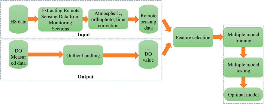
FIGURE 2. Technical Roadmap.

2.3.3 Model framework

The paper proposes a DO-MDNN (Dissolved Oxygen Multimodal Deep Neural Network) model, which consists of four single-modal neural networks (sNNs). Here, sNN refers to an independent neural network corresponding to each perception modal in the multimodal neural network. Each sNN processes its respective input data and extracts useful information from the multimodal data through a fusion or integration mechanism, as illustrated in Figure 3. The model is designed with one sNN for each modal, allowing the model to effectively balance information and noise during the training phase. Modal A, Modal B, and Modal C represent remote sensing data. The outputs of Subnetwork 1 (sNN1), Subnetwork 2 (sNN2), and Subnetwork 3 (sNN3) are non-linearly mapped through a weighted sum in the hidden layer to obtain the input features, which are then connected to Subnetwork 4 (sNN4) for DO inversion. The number of neurons in each layer of the network is labeled in Figure 3 to illustrate the model structure.

FIGURE 3

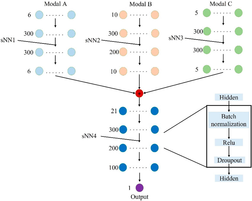
FIGURE 3. The model network structure diagram.

2.3.4 Structure and parameter determination

In Figure 3, sNN1, sNN2, and sNN3 are all set as neural networks with three hidden layers, while sNN4 is set as a neural network with four hidden layers. The number of neurons in the input layer of sNN1, sNN2, and sNN3 depends on the features number in each modal, while the number of neurons in the output layer is determined based on the model’s performance.

To prevent overfitting, a Batch Normalization (BN) layer, a Rectified Linear Unit (ReLU) activation function, and a dropout layer are added after each hidden layer. The BN layer and dropout layer serve to normalize the features and discard some neurons in the network to improve the generalization ability of the inversion model. During the training process, the three modalities are trained separately in sNN1, sNN2, and sNN3, and their outputs are then concatenated (represented by the red nodes in Figure 3) and fed into sNN4 for further training. In terms of model optimization, Mean Squared Error Loss (MSELoss) is used as the optimization parameter (Eq. 8), and the Adaptive Moment Estimation (Adam) optimizer is employed for gradient descent.

$\mathit{M}\mathit{S}\mathit{E}\mathit{L}\mathit{o}\mathit{s}\mathit{s}=\frac{\mathbf{1}}{\mathit{n}}{\displaystyle \sum _{\mathit{i}=\mathbf{1}}^{\mathit{n}}}{\left({\mathit{y}}_{\mathit{i}}-\widehat{{\mathit{y}}_{\mathit{i}}}\right)}^{\mathbf{2}}(8)$

Where $y_i$ and $\widehat{y_i}$ represent the observed and inverted DO concentrations, respectively, and $n$ denotes the number of samples.

2.3.5 Comparison with other models

In this study, 80% of the data was randomly allocated for training the model (N = 5940), and the remaining 20% of the data was used as the test set for model evaluation (N = 1489).

In this study, six machine learning algorithms, namely, ElasticNet, K-Nearest Neighbors (KNN), Support Vector Regression (SVR) (e.g., Guo et al., 2021), Random Forest (RF) (e.g., Cao et al., 2020), Extreme Gradient Boosting (XGBoost) (e.g., Bui et al., 2020), and Light Gradient Boosting Machine (LightGBM), were used as comparative models. The same data partitioning method was applied to all algorithms, and a Genetic Algorithm (GA) was used to search for the optimal hyperparameters relative to each model.

2.3.6 Model evaluation

To quantitatively describe the inversion capability of the DO inversion model, this chapter utilizes multiple indicators to evaluate its performance. These indicators include adj_R², Root Mean Square Error (RMSE), Percent bias (Pbias) (e.g., Bui et al., 2020) and Symmetric Mean Absolute Percentage Error (SMAPE) (e.g., Zaini et al., 2021a). The calculation formulas, value ranges, and optimal values for these evaluation indicators are presented in Table 3.

TABLE 3

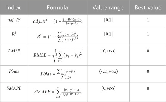
TABLE 3. Calculation formula, value range, and optimal value of evaluation indicators.

Where $R^2$ is the coefficient of determination between the simulated values and the measured values, $y_i$ represents the i-th variable of the measured DO, $\overline{y}$ is the average value of the measured DO, $\widehat{y_i}$ represents the i-th variable of the simulated DO, n is the number of samples, and p is the number of features.

3 Result

3.1 Statistical analysis of measured DO

Figure 4 displays the monthly average DO concentrations from 2019 to 2021. The original DO concentrations in the monitoring sections of Lake Taihu exhibit evident seasonal variations. The MK trend test reveals a significant decreasing trend in DO concentrations during spring (March to May) (p < 0.01) and a significant increasing trend during autumn (September to November) (p < 0.01). DO concentrations in summer (June to August) are lower than in winter (December to February of the following year), with varying trends across different years, indicating substantial inter-seasonal variations. The range of DO concentrations throughout the year is 6–14 mg/L, with the lowest average values observed in summer and the highest average values occurring during the colder winter months, suggesting uneven seasonal distribution of DO concentrations in the monitored sections of Lake Taihu, likely influenced by temperature. Pearson correlation analysis indicates a significant negative correlation between DO concentrations and water temperature in the monitoring sections, with a Pearson coefficient of −0.81 and p-value <0.01.

FIGURE 4

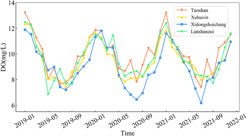
FIGURE 4. Monthly Average Trends of DO Concentration from 2019 to 2021.

Regarding spatial heterogeneity, the Tuoshan monitoring section shows higher overall DO concentrations, with an average DO concentration of 9.99 mg/L from January 2019 to December 2021. On the other hand, the Xidongshuichang monitoring section exhibits lower overall DO concentrations, with an average DO concentration of 9.10 mg/L during the same period. In general, DO concentrations in the western part of Lake Taihu are slightly higher than in the eastern part, especially during winter, where Tuoshan and Lanshanzui sections have relatively higher DO concentrations. These findings indicate the presence of spatial heterogeneity among the four monitoring sections in Lake Taihu.

3.2 Feature selection

After merging the DO concentrations from the four monitoring sections, the correlation between all remote sensing features and DO concentrations was examined using the Pearson correlation analysis method. Table 4 displays pearson correlation coefficient between DO and various characteristics, indicating the feasibility of using remote sensing information such as visible, near-infrared, and shortwave infrared bands of Rrs, spectral indices, and surface temperature in the infrared band for DO concentration inversion.

TABLE 4

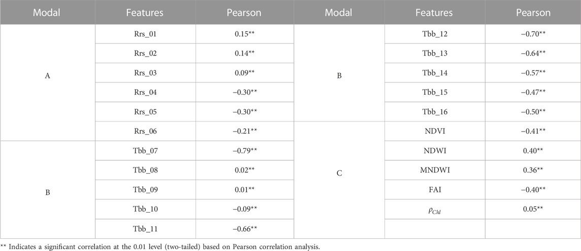
TABLE 4. Pearson correlation coefficient between DO and various characteristics.

3.3 Model performance

The evaluation results on the test set were chosen to represent the model’s performance in practical applications. Firstly, six machine learning models were used to compare the effectiveness of the DO-MDNN method. As shown in Figure 5, the LightGBM model demonstrated the best performance among the six models, with adj_R², RMSE, SMAPE, and Pbias values of 74.18%, 0.70 mg/L, 5.94%, and −0.007% respectively. On the other hand, the ElasticNet model showed the poorest performance, with adj_R², RMSE, SMAPE, and Pbias values of 69.73%, 0.76 mg/L, 6.61%, and −0.003% respectively. Using the same dataset, we trained and validated the DO-MDNN model developed in this study to further investigate its advantages. As illustrated in Figure 6, the DO-MDNN model developed in this study provided more accurate DO concentration estimations (adj_R², RMSE, SMAPE, and Pbias values of 77.11%, 0.66 mg/L, 5.36%, and −0.44% respectively), as expected. The evaluation results indicated that the DO-MDNN model outperformed all other models. Compared to the average performance of the other baseline models, DO-MDNN showed a 6.40% increase in adj_R², an 8.27% reduction in RMSE, and a 12.1% decrease in SMAPE. The density plot shown in Figure 6 visually demonstrates the performance of the DO-MDNN model’s DO estimations compared to the actual measurements on the test set, effectively avoiding data stacking issues.

FIGURE 5

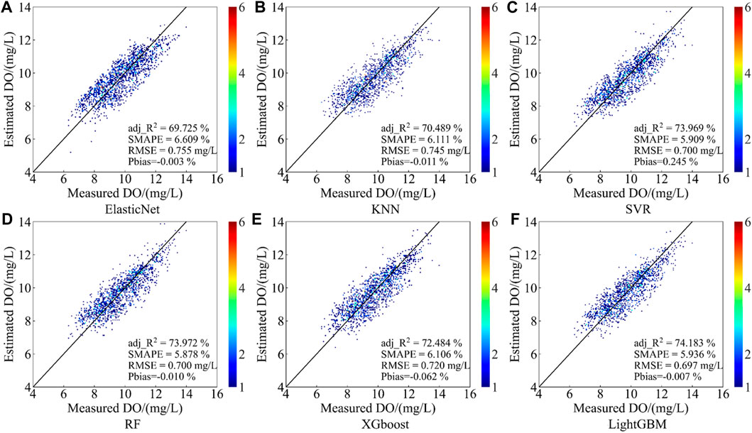
FIGURE 5. Fitting Plots of Six Machine Learning Models.

FIGURE 6

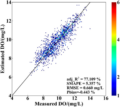
FIGURE 6. Fitting Plot of the DO-MDNN Model.

Therefore, the DO -MDNN model developed in this study has been demonstrated to successfully invert DO concentration using H8 satellite data and can be used for high-frequency dynamic monitoring of DO.

In order to verify the application of the DO-MDNN model in the whole Lake Taihu region, we selected the H8 data from 08:00-13:00 on May 16, 2022, and mapped the DO concentration in the Lake Taihu region on a time-by-time basis, and the results are shown in Figure 7. DO concentration varied from 8.5 to 11.5 mg/L from 8:00 to 13:00, with an overall increase and then a decrease in DO concentration values, with an overall increase in DO concentration values from 8:00 to 10:00, and a beginning of a decrease in DO concentration values from 11:00 to 13:00, especially in littoral areas such as the southwestern and northeastern parts of the country. The southwestern part of Lake Taihu is mostly the river inlet, with vigorous vegetation and shallow water nearby leading to strong photosynthesis and higher DO concentrations. The northeastern part of Lake Taihu is mainly an economically developed urban area with a large population density, which is affected by anthropogenic factors all year round, and the littoral areas of the lake are in a state of nutrient fertilization all year round, resulting in a higher DO concentration. The above results show that the DO-MDNN model has some applicability in the Taihu Lake region.

FIGURE 7

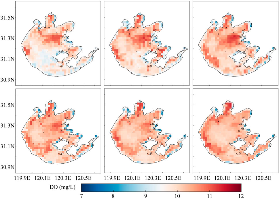
FIGURE 7. Remote sensing mapping of DO concentrations in the Lake Taihu region from 08:00 to 13:00 (order is from top left to bottom right).

4 Discussion

4.1 Model advantages and limitations

4.1.1 Model advantages

(1) The DO-MDNN model constructed in this study validates the feasibility of using geostationary satellite remote sensing data for the inversion of non-optical active parameter, DO concentration. The model demonstrates high accuracy and provides reliable data support for lake water quality inversion using geostationary satellite data, which complements the limitations of traditional water quality monitoring and estimation. It offers advantages such as wide coverage, rapid monitoring, and addresses the low revisit rate of polar-orbiting satellites, thereby enhancing the current level of water environment protection and management.

(2) Firstly, this model divides the input features into three modalities, enabling the model to capture multimodal information. Each modality can focus on extracting and learning specific types of features, thus reflecting the influencing factors of DO more comprehensively. Secondly, the adoption of multimodal neural networks allows for the full utilization of the expressive capabilities of each modality. Through hierarchical feature extraction and combination, the model enhances its ability to represent the input features and better learn the complex relationship between DO and these features. Finally, different modalities of features may possess distinct scales, distributions, and correlations. By handling them separately, the model can reduce interference during the learning process. Moreover, multimodal neural networks can effectively learn correlations between different modalities through appropriate weight sharing and joint training, thereby improving the model’s generalization ability.

(3) The H8 satellite data inversion model not only shows technical advantages in DO monitoring, but also has the potential to be extended to other water quality indicators, such as total phosphorus and total nitrogen. Specific spectral channels may capture optical features associated with total phosphorus and total nitrogen concentrations, such as particulate matter concentrations, the presence of nitrogen compounds, and the color of the water column. In addition, changes in temperature distribution and biological activity may also be affected by total nitrogen. Through in-depth research and model development, we can further explore how to effectively utilize H8 data as well as deep learning models to enable remote monitoring and estimation of key water quality indicators such as total phosphorus and total nitrogen, which can provide important support for water resource management and ecosystem monitoring.

4.1.2 Model limitations

The discrepancy between the model’s output and the true values can be attributed to several factors. Firstly, the water quality parameters are collected from fixed monitoring points, while the spatial resolution of the satellite data used in this study is relatively low (2 km). As a result, the presence of other interfering factors within the same remote sensing pixel adds complexity and makes it challenging to achieve a perfect match. Secondly, the DO concentrations outputted by the proposed DO inversion model represent average values within the remote sensing pixel and may not directly correspond to the measured concentrations at automatic monitoring stations. The proximity to the land adjacency effect (e.g., Sun et al. 2022) negatively impacts the inversion results, with poorer performance observed in areas closer to the lake shore (e.g., Zhao et al. 2021). Additionally, the measurements taken at automatic monitoring stations may be affected by unexpected events such as changes in sensor environment, network failures, or the presence of boats and fish. Furthermore, remote sensing satellites are unable to monitor the vertical profiles of water bodies, and different water bodies exhibit significant individual variations in their optical properties. All of these factors can contribute to certain errors in water quality inversion and prediction.

4.2 Reasons for the uneven distribution of DO over time

Based on the analysis of DO measured data over time, it is evident that the DO concentration in Lake Taihu exhibits an uneven temporal distribution, with higher levels observed in summer and autumn compared to spring and winter. This phenomenon is likely attributed to several factors. During the summer and autumn, local water temperature rises, and there is abundant sunlight, leading to significant reproduction of aquatic organisms. Additionally, increased rainfall in summer results in a higher influx of pollution loads into Lake Taihu, leading to eutrophication and increased DO consumption, thereby causing higher-than-normal occurrences of cyanobacterial blooms and a gradual decline in water quality (e.g., Dai et al., 2020). In the winter, the Lake Taihu ecosystem enters a dormant state, although some aquatic organisms remain active due to the subtropical monsoon climate of the region (e.g., Lyu et al., 2015). Cyanobacterial frequency decreases during this period, resulting in gradually higher DO content in the water. As a result, the correlation between DO concentration and cyanobacterial blooms becomes weaker during non-blooming periods, while during cyanobacterial bloom outbreaks, there is a negative correlation between DO concentration and the frequency of bloom events. Rapid increases in cyanobacterial populations lead to a large amount of photosynthesis, depleting DO levels in the water. Moreover, after cyanobacteria die, they also consume oxygen, further reducing the DO concentration in the water. Hence, cyanobacterial bloom periods are often associated with lower DO concentrations in the water. These combined factors result in the uneven temporal distribution of DO concentrations in Lake Taihu during different seasons. Analyzing the spatiotemporal distribution changes of non-optical active parameters in different research areas is crucial for improving the precision of remote sensing inversion of non-optical active parameters.

4.3 Comparison of models based on time series decomposition

In typical situations, during the training of a machine learning model, the high correlation between the input and output data may be due to both exhibiting simultaneous upward or downward trends in time, rather than a true fit. This phenomenon is particularly evident in time series data. If the trend component (a persistent upward or downward movement or state that develops over a long period) and the seasonal component (regular variations in the level of development caused by seasonal changes) cannot be eliminated, it becomes challenging to accurately map features in residual analysis. This is also referred to as the “spurious regression” phenomenon (e.g., Tian, 2014).

This study takes the “Xuhuxin” section as an example. Due to the longer data sequence of this site, it was chosen as the research object. The measured DO data can be treated as a time series $Y\left(t\right)$, and the Seasonal and Trend decomposition using Loess (STL) algorithm (e.g., Rojo et al., 2017) is used to decompose it.

$\mathit{Y}\left(\mathit{t}\right)=\mathit{S}\left(\mathit{t}\right)+\mathit{T}\left(\mathit{t}\right)+\mathit{R}\left(\mathit{t}\right)(9)$

Where $Y\left(t\right)$ represents the DO concentration at time $t$, $S\left(t\right)$ represents the periodic component at time $t$, $T\left(t\right)$ represents the trend component at time $t$, and $R\left(t\right)$ represents the residual component at time $t$. The time series $Y\left(t\right)$ exhibit a fixed “annual cycle” $S_{year}\left(t\right)$ over the course of a year and a fixed “daily cycle” $S_{day}\left(t\right)$ within a day. The parameters for the annual cycle are set as $n_{p-year}$ = 365 days, and for the daily cycle as $n_{p-day}$ = 24 h. Since a single STL decomposition can only extract one type of periodic component, the first step is to remove the annual cycle component $S_{year}\left(t\right)$ from $Y\left(t\right)$ to obtain a new time series $X_1\left(t\right)$ without the annual cycle. Then, the daily cycle component $S_{day}\left(t\right)$ is removed from $X_1\left(t\right)$ to obtain the combined trend and residual components of the DO measured data in the series $X_2\left(t\right)$.

The Augmented Dickey-Fuller (ADF) test (e.g., Zaini et al., 2021b) is applied to the merged component $X_2\left(t\right)$ to check for stationarity. If $X_2\left(t\right)$ is not stationary, differencing will be performed. If $X_2\left(t\right)$ is stationary, a white noise test will be conducted. If $X_2\left(t\right)$ is a white noise sequence, it indicates that the data is invalid and the experiment should be stopped. If $X_2\left(t\right)$ is a stationary non-white noise sequence, it implies that the output data has eliminated periodic variations, and $X_2\left(t\right)$ can be used as the output for model construction in the next section.

The evaluation results on the test set were chosen to represent the model’s performance in practical applications. Firstly, six machine learning models were used to compare the effectiveness of the STL method. The merged component $X_2\left(t\right)$ obtained from the second STL decomposition of DO concentration was used as the model output, and the performance of the models before and after STL decomposition was compared. As shown in Figure 8 and Table 5, the comparison models after STL processing exhibited significant improvements compared to the models without STL decomposition. The average adj_R² of the six machine learning models increased by 0.26, RMSE decreased by 0.24 mg/L, and SMAPE decreased by 2.2% after STL processing. Among them, the ElasticNet model showed the largest improvement in the comparison before and after STL decomposition, with a difference of 0.19 in adj_R², 0.23 mg/L in RMSE, and 1.56% in SMAPE, indicating a significant enhancement in its performance. Meanwhile, the DO-MDNN model showed an increase of 0.14 in adj_R², a decrease of 0.23 mg/L in RMSE, and a decrease of 2.1% in SMAPE after STL decomposition. The above results demonstrate that STL decomposition helps remove noise and trend components from the DO concentration time series, thereby improving the accuracy of DO inversion.

FIGURE 8

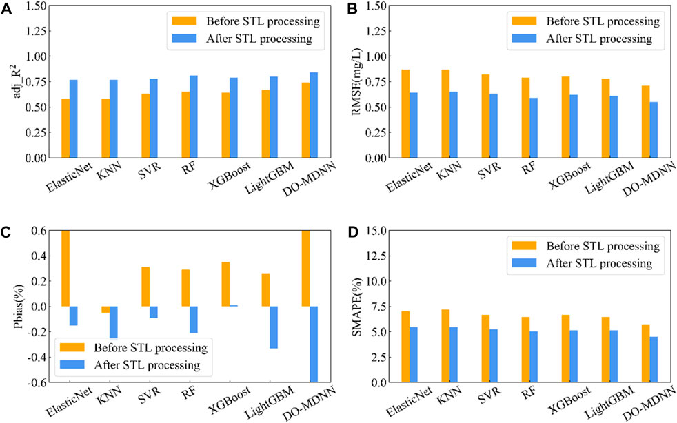
FIGURE 8. Comparison plots of each model before and after STL processing.

TABLE 5

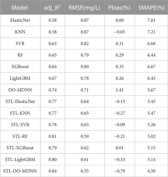
TABLE 5. Comparison of each model before and after STL processing.

The model constructed in this section is specifically designed for the single observation station “Xuhuxin” and does not have the feasibility to be applied to other areas within Lake Taihu or other water bodies outside of Lake Taihu. In this study, only the time series of the “Xuhuxin” site were relatively complete for the four sites, while the time series of the other three sites were not complete enough. Therefore, the accuracy of the removed periodic terms in the overall time series decomposition cannot be determined. Therefore, this study only used the “Xuhuxin” site. In practical applications, it is necessary to increase the number of DO observation stations and establish a unified model that fits all DO observation stations. Only then can we consider the model to be applicable to the water bodies represented by these DO observation stations.

4.4 Optical basis for remote sensing inversion methods

In the field of water ecology and bio-optics, the optical mechanism and bio-optical processes of DO are of great significance for monitoring and analyzing ecosystems, and the H8 satellite plays a key role in this regard. DO, as the dissolved state of oxygen in water, is essential for sustaining aquatic organisms. Optical analysis methods, such as oxygen sensors, utilize the H8 satellite’s high-resolution optical sensors to achieve accurate measurements of DO concentration through the interaction of fluorescence or absorption properties with oxygen molecules. At the same time, the H8 satellite monitored the refraction and reflection of light on the surface of water bodies, providing important data for processes such as photosynthesis and oxygen dissolution. In addition, the H8 satellite was able to capture the temperature distribution of the water body, helping us to understand the effect of light on the interrelationship between temperature and oxygen solubility. In summary, the optical mechanism and bio-optical processes of DO are integrated with the H8 satellite observation data, which will help to explore the dynamics of aquatic ecosystems in depth and provide scientific support for ecological protection and sustainable management.

Among them, Tbb_07, Tbb_08, Tbb_10, Tbb_12 as infrared bands are mainly used to invert the water temperature (e.g., Yamamoto et al., 2018), and the correlation between the water temperature and DO is high (e.g., Rajwa-Kuligiewicz et al., 2015), so Tbb_07, Tbb_08, Tbb_10, and Tbb_12 have strong correlation to DO in this study; MNDWI (e.g., Guha and Govil, 2022), ${\rho }_{Chl}$ (e.g., Feng et al., 2022) and others as spectral indices are assess the vegetation growth condition by calculating the ratio between the reflectance of red, near-infrared and blue light bands, so it can indirectly reflect the concentration of DO; Wang, et al. (2013) pointed out that DO was negatively correlated with the remote sensing reflectance with the center wavelength in the range of 400-900 nm, and the highest correlation was found at 686 nm, and the center wavelength of Rrs_03 was 640 nm, and the correlation to the DO The center wavelength of Rrs_03 is 640 nm, and the correlation of Rrs_03 to DO is stronger, which is consistent with the conclusion of its research; Rrs_06 and Rrs_05 mainly invert environmental parameters such as vegetation index (e.g., Wang et al., 2022b), soil moisture, surface temperature, etc., which are indirectly related to DO, and therefore the correlation of Rrs_06 and Rrs_05 to DO is also higher.

5 Conclusion

With the rapid development of artificial intelligence and remote sensing technology, the application of machine learning or deep learning models in the inversion and prediction of lake water quality has become a hot topic in the interdisciplinary field of artificial intelligence and environment. The process of obtaining traditional water quality indicators is time-consuming and labor-intensive, often requiring on-site collection of water samples, appropriate storage, and transportation to laboratories for testing. Even data generated by automatic monitoring stations may have some defects. To address the shortcomings of traditional water quality monitoring, this study combines a large amount of historical monitoring water quality data with satellite remote sensing data and uses the DO-MDNN model to achieve more frequent and macroscopic monitoring activities. This approach has the advantages of wide coverage and fast monitoring, providing an effective reference for improving the level of water environment monitoring and holding significant importance for protecting lake water quality. The conclusions of this research are as follows:

(1) Based on H8 data and DO measured data, a deep learning method was employed to propose a DO inversion model called DO-MDNN. The results showed that the average performance of the DO-MDNN model was adj_R² of 0.77, RMSE of 0.66 mg/L, Pbias of −0.44%, and SMAPE of 5.36%. Compared to other baseline models, DO-MDNN exhibited better average performance, with a 6.40% increase in adj_R², an 8.27% decrease in RMSE, and a 12.1% decrease in SMAPE.

(2) The comparison models after STL processing exhibited significant improvement compared to the models without STL decomposition. The six machine learning models showed an average increase of 0.26 in adj_R², a decrease of 0.24 mg/L in RMSE, and a decrease of 2.2% in SMAPE. Among them, the ElasticNet model showed the largest difference in the before and after STL decomposition comparison, with a 0.19 difference in adj_R², a 0.23 mg/L difference in RMSE, and a 1.56% difference in SMAPE, showing a significantly improved performance. Additionally, the DO-MDNN model had an increase of 0.14 in adj_R², a decrease of 0.23 mg/L in RMSE, and a decrease of 2.1% in SMAPE compared to before STL decomposition. The above results indicate that STL decomposition helps remove noise and trend components from the DO concentration time series, thereby enhancing the accuracy of DO inversion.

(3) Based on the H8 data, DO measurements, and the DO-MDNN model, it is possible to achieve hourly monitoring of DO concentration. This capability meets the demand for high-frequency and dynamic monitoring of DO concentration, providing strong support for marine environmental management and conservation efforts.

Data availability statement

Publicly available datasets were analyzed in this study. This data can be found here: Himawari-8 data from https://www.eorc.jaxa.jp/ptree/ Water quality data from Chinese Research Academy of Environmental Sciences.

Author contributions

KS and QL designed the research. WY and PW conducted experiments and developed models. KS and WY analyzed the result and wrote the manuscript. QL reviewed and edited the manuscript. All authors contributed to the article and approved the submitted version.

Funding

This work was supported by the Key Research Project of Qinghai Province (2021-SF-A7-1), the National Key Research and Development Program (2021YFC310170504) and the Research Project on Machine Learning-based Satellite Remote Sensing for Multi-index Water Quality Inversion, Monitoring, and Early Warning Technology of the State Key Laboratory of Ecological and Agricultural on the Qinghai-Tibet Plateau (2023-ZZ-09).

Conflict of interest

The authors declare that the research was conducted in the absence of any commercial or financial relationships that could be construed as a potential conflict of interest.

Publisher’s note

All claims expressed in this article are solely those of the authors and do not necessarily represent those of their affiliated organizations, or those of the publisher, the editors and the reviewers. Any product that may be evaluated in this article, or claim that may be made by its manufacturer, is not guaranteed or endorsed by the publisher.

References

Batur, E., and Maktav, D. (2018). Assessment of surface water quality by using satellite images fusion based on PCA method in the Lake Gala, Turkey. IEEE Trans. Geoscience Remote Sens. 57 (5), 2983–2989. doi:10.1109/TGRS.2018.2879024

CrossRef Full Text | Google Scholar

Bui, D. T., Khosravi, K., Tiefenbacher, J., Nguyen, H., and Kazakis, N. (2020). Improving prediction of water quality indices using novel hybrid machine-learning algorithms. Sci. Total Environ. 721, 137612. doi:10.1016/j.scitotenv.2020.137612

PubMed Abstract | CrossRef Full Text | Google Scholar

Cao, Z. G., Ma, R. H., Duan, H. T., Pahlevan, N., Melack, J., Shen, M., et al. (2020). A machine learning approach to estimate chlorophyll-a from Landsat-8 measurements in inland lakes. Remote Sens. Environ. 248, 111974. doi:10.1016/j.rse.2020.111974

CrossRef Full Text | Google Scholar

Changzhou Ecological Environment Bureau, (2021). Suzhou ecological environment status bulletin. Changzhou, China: Changzhou Ecological Environment Bureau.

Google Scholar

Chen, J., and Quan, W. T. (2012). Using landsat/TM imagery to estimate nitrogen and phosphorus concentration in Taihu Lake, China. IEEE J. Sel. Top. Appl. Earth Observations Remote Sens. 5 (1), 273–280. doi:10.1109/jstars.2011.2174339

CrossRef Full Text | Google Scholar

Chen, J., Zheng, W., Wu, S., Liu, C., and Yan, H. (2022). Fire monitoring algorithm and its application on the geo-kompsat-2A geostationary meteorological satellite. Remote Sens. 14 (11), 2655. doi:10.3390/RS14112655

CrossRef Full Text | Google Scholar

Chen, N. W., Yu, Y. Q., Chen, J. X., Chen, L. B., and Zhang, D. Z. (2021). Artificial neural network models for water quality early warning: A review. Acta Sci. Circumstantiae 41 (12), 4771–4782. doi:10.13671/j.hjkxxb.2021.0343

CrossRef Full Text | Google Scholar

Chen, X. R. (2019). High-frequency observation of floating algae bloom from AHI on himawari-8. Xiamen, China: Xiamen University.

Google Scholar

Dai, Q. Z., Zhang, K., and Xu, B. (2020). The trend of water quality variation and analysis of meiliang bay and dongtaihu bay in Taihu Lake from 2014 to 2018. China Rural Water Hydropower (7), 82–84.

Google Scholar

Feng, T. S., Pang, Z. G., and Jiang, W. (2022). Remote sensing retrieval of chlorophyll-a concentration in Lake chaohu based on zhuhai-1 hyperspectral satellite. Spectrosc. Spectr. Analysis 42 (8), 2642–2648. doi:10.3964/j.issn.1000-0593(2022)08-2642-07

CrossRef Full Text | Google Scholar

Guha, S., and Govil, H. (2022). Annual assessment on the relationship between land surface temperature and six remote sensing indices using landsat data from 1988 to 2019. Geocarto Int. 37 (15), 4292–4311. doi:10.1080/10106049.2021.1886339

CrossRef Full Text | Google Scholar

Guo, H. W., Tian, S., Huang, J. .H. J. .N., Zhu, X. T., Wang, B., and Zhang, Z. J. (2022). Performance of deep learning in mapping water quality of Lake Simcoe with long-term Landsat archive. ISPRS J. Photogrammetry Remote Sens. 183, 451–469. doi:10.1016/j.isprsjprs.2021.11.023

CrossRef Full Text | Google Scholar

Guo, H. W., Huang, J. J., Zhu, X. T., Wang, B., Tian, S., Xu, W., et al. (2021). A generalized machine learning approach for dissolved oxygen estimation at multiple spatiotemporal scales using remote sensing. Environ. Pollut. 288, 117734. doi:10.1016/J.ENVPOL.2021.117734

PubMed Abstract | CrossRef Full Text | Google Scholar

Hersbach, H., Bell, B., Berrisford, P., Hirahara, S., Horanyi, A., Munoz-Sabater, J., et al. (2020). The ERA5 global reanalysis. Q. J. R. Meteorological Soc. 146 (730), 1999–2049. doi:10.1002/qj.3803

CrossRef Full Text | Google Scholar

Karakaya, N., and Evrendilek, F. (2011). Monitoring and validating spatio-temporal dynamics of biogeochemical properties in Mersin Bay (Turkey) using Landsat ETM+. Environ. Monit. Assess. 181, 457–464. doi:10.1007/s10661-010-1841-5

PubMed Abstract | CrossRef Full Text | Google Scholar

Kim, Y. H., Son, S., Kim, H. C., Kim, B., Park, Y. G., Nam, J., et al. (2020). Application of satellite remote sensing in monitoring dissolved oxygen variabilities: A case study for coastal waters in korea. Environ. Int. 134, 105301. doi:10.1016/j.envint.2019.105301

PubMed Abstract | CrossRef Full Text | Google Scholar

Li, Y., Li, Y. M., Wang, Q., Zhu, L., and Guo, Y. L. (2014). An observing system simulation experiments framework based on the ensemble square root kalman filter for evaluating the concentration of chlorophyll a by multi-source data: A case study in Taihu Lake. Aquatic Ecosyst. Health & Manag. 17 (3), 233–241. doi:10.1080/14634988.2014.940799

CrossRef Full Text | Google Scholar

Liang, Y. C., Yin, F., Zhao, Y. F., and Liu, L. (2021). Remote sensing inversion of biochemical oxygen demand in Taihu Lake based on Landsat 8 images. Ecol. Environ. Sci. 30 (7), 1492–1502. doi:10.16258/j.cnki.1674-5906.2021.07.018

CrossRef Full Text | Google Scholar

Liu, P., Wang, J., Sangaiah, A. K., Xie, Y., and Yin, X. C. (2019). Analysis and prediction of water quality using LSTM deep neural networks in IoT environment. Sustainability 11 (7), 2058. doi:10.3390/su11072058

CrossRef Full Text | Google Scholar

Lyu, H., Zhang, J., Zha, G. H., Wang, Q., and Li, Y. M. (2015). Developing a two-step retrieval method for estimating total suspended solid concentration in Chinese turbid inland lakes using Geostationary Ocean Colour Imager (GOCI) imagery. Int. J. Remote Sens. 36 (5), 1385–1405. doi:10.1080/01431161.2015.1009654

CrossRef Full Text | Google Scholar

Ma, R. H., Duan, H. T., Gu, X. H., and Zhang, S. X. (2008). Detecting aquatic vegetation changes in Taihu Lake, China using multi-temporal satellite imagery. Sensors 8 (6), 3988–4005. doi:10.3390/s8063988

PubMed Abstract | CrossRef Full Text | Google Scholar

Ma, Z. M., Niu, Y., Xie, P., Chen, J., Tao, M., and Deng, X. W. (2013). Off-flavor compounds from decaying cyanobacterial blooms of Lake Taihu. J. Environ. Sci. 25 (3), 495–501. doi:10.1016/S1001-0742(12)60101-6

PubMed Abstract | CrossRef Full Text | Google Scholar

Ngiam, J., Khosla, A., Kim, M., Nam, J., Lee, H., and Ng, A. Y. (June 2018). Multimodal deep learning. Proceedings of the international conference on machine learning, Bellevue Washington USA,

Google Scholar

Ning, H. T., Jiang, P., and Wu, Y. L. (2021). Research on aerosol optical depth retrieval of himawari-8 data based on deep neural networks. Adm. Tech. Environ. Monit. 33 (1), 8–12. doi:10.19501/j.cnki.1006-2009.2021.01.003

CrossRef Full Text | Google Scholar

Peterson, K. T., Sagan, V., and Sloan, J. J. (2020). Deep learning-based water quality estimation and anomaly detection using Landsat-8/Sentinel-2 virtual constellation and cloud computing. GIScience Remote Sens. 57 (4), 510–525. doi:10.1080/15481603.2020.1738061

CrossRef Full Text | Google Scholar

Qi, L., Hu, C. M., Duan, H. T., Cannizzaro, j., and Ma, R. H. (2014). A novel MERIS algorithm to derive cyanobacterial phycocyanin pigment concentrations in a eutrophic lake: Theoretical basis and practical considerations. Remote Sens. Environ. 154, 298–317. doi:10.1016/j.rse.2014.08.026

CrossRef Full Text | Google Scholar

Rajwa-Kuligiewicz, A., Bialik, R. J., and Rowinski, P. M. (2015). Dissolved oxygen and water temperature dynamics in lowland rivers over various timescales. J. HYDROLOGY HYDROMECHANICS 63 (4), 353–363. doi:10.1515/johh-2015-0041

CrossRef Full Text | Google Scholar

Rojo, J., Rivero, R., Romero-Morte, J., Fernandez-Gonzalez, F., and Perez-Badia, R. (2017). Modeling pollen time series using seasonal-trend decomposition procedure based on LOESS smoothing. Int. J. Biometeorol. 61 (2), 335–348. doi:10.1007/s00484-016-1215-y

PubMed Abstract | CrossRef Full Text | Google Scholar

Sagan, V., Peterson, K. T., Maimaitijiang, M., Sidike, P., Sloan, J., Greeling, B. A., et al. (2020). Monitoring inland water quality using remote sensing: Potential and limitations of spectral indices, bio-optical simulations, machine learning, and cloud computing. Earth-Science Rev. 205, 103187. doi:10.1016/j.earscirev.2020.103187

CrossRef Full Text | Google Scholar

Sharaf, El. D. E., Zhang, Y., and Suliman, A. (2017). Mapping concentrations of surface water quality parameters using a novel remote sensing and artificial intelligence framework. Int. J. Remote Sens. 38 (4), 1023–1042. doi:10.1080/01431161.2016.1275056

CrossRef Full Text | Google Scholar

Sun, X., Zhang, Y. L., Shi, K., Zhang, Y. B., Li, N., Wang, W. J., et al. (2022). Monitoring water quality using proximal remote sensing technology. Sci. Total Environ. 803, 149805. doi:10.1016/J.SCITOTENV.2021.149805

PubMed Abstract | CrossRef Full Text | Google Scholar

Suzhou Ecological Environment Bureau, (2021). Suzhou ecological environment status bulletin. Suzhou, China: Suzhou Ecological Environment Bureau.

Google Scholar

Tian, L. F. (2014). Analysis of the "pseudo regression" of non stationary data. Statistics Decis. Mak. 39 (3), 17–21. doi:10.13546/j.cnki.tjyjc.000004

CrossRef Full Text | Google Scholar

Wang, B., An, H. J., and Lv, C. W. (2013). Inversion modeling of dissolved oxygen in Hulun Lake of Northeast China based on multisource remote sensing. Chin. J. Ecol. 32 (4), 993–998. doi:10.13292/j.1000-4890.2013.0174

CrossRef Full Text | Google Scholar

Wang, G., Wang, D. Y., and Wu, R. (2020). Application study of Himawari-8/AHI ionfrared spectral data on precipitation signal recognition and retrieval. J.Infrared Millim. Waves. 39 (02), 251–262. doi:10.11972/j.issn.1001-9014.2020.02.013

CrossRef Full Text | Google Scholar

Wang, M., Zheng, W., and Liu, C. (2017). Application of Himawari-8 data with high-frequency observation for Cyanobacteria bloom dynamically monitoring in Lake Taihu. J. Lake Sci. 29 (05), 1043–1053. doi:10.18307/2017.0502

CrossRef Full Text | Google Scholar

Wang, X. X., Lu, X. P., and Li, G. Q. (2022b). Extracting urban vegetation information by combining the red edge near red vegetation index with DEM. Spectrosc. Spectr. Analysis 42 (7), 2284–2289. doi:10.3964/J.ISSN.1000-0593(2022)07-2284-06

CrossRef Full Text | Google Scholar

Wang, Z. C., Wang, J., Yan, S. J., Cui, Y. H., and Wang, H. H. (2022a). Annual dynamic remote sensing monitoring of phycocyanin concentration in Lake Chaohu based on Sentinel-3 OLCI images. J. Lake Sci. 34 (2), 391–403. doi:10.18307/2022.0203

CrossRef Full Text | Google Scholar

Wuxi Ecological Environment Bureau, (2021). Suzhou ecological environment status bulletin. Wuxi, City: Wuxi Ecological Environment Bureau.

Google Scholar

Yamamoto, Y., Ishikawa, H., Oku, Y., and Hu, Z. (2018). An algorithm for land surface temperature retrieval using three thermal infrared bands of himawari-8. J. METEOROLOGICAL Soc. Jpn. 96 (B), 59–76. doi:10.2151/jmsj.2018-005

CrossRef Full Text | Google Scholar

Yang, J. Y., Zhang, S., Bai, Y., Huang, A. Q., and Zhang, J. H. (2021). SPEI simulation for monitoring drought based machine learning integrating multi-source remote sensing data in shandong. Chin. J. Agrometeorology 42 (3), 230–242. doi:10.3969/j.issn.1000-6362.2021.03.007

CrossRef Full Text | Google Scholar

Zaini, N., Ean, L. W., Ahmed, A. N., and Malek, M. A. (2021a). A systematic literature review of deep learning neural network for time series air quality forecasting. Environ. Sci. Pollut. Res. 29 (4), 4958–4990. doi:10.1007/S11356-021-17442-1

CrossRef Full Text | Google Scholar

Zaini, N., Ean, L. W., Ahmed, A. N., and Malek, M. A. (2021b). A systematic literature review of deep learning neural network for time series air quality forecasting. Environ. Sci. Pollut. Res. 29 (4), 4958–4990. doi:10.1007/s11356-021-17442-1

CrossRef Full Text | Google Scholar

Zhang, H. J., Wang, B., Zhou, J., Yu, Y., Ke, S., and Huang, F. K. (2022). Remote sensing retrieval of inland river water quality based on BP neural network. J. Central China Normal Univ. Sci. 56 (02), 333–341. doi:10.19603/j.cnki.1000-1190.2022.02.017

CrossRef Full Text | Google Scholar

Zhang, Y. C., Lin, S., Liu, J. P., Qian, X., and Ge, Y. (2010). Time-series MODIS image-based retrieval and distribution analysis of total suspended matter concentrations in Lake Taihu (China). Int. J. Environ. Res. Public Health 7 (9), 3545–3560. doi:10.3390/IJERPH7093545

PubMed Abstract | CrossRef Full Text | Google Scholar

Zhao, X. L., Xu, H. L., Ding, Z. B., Wang, D. Q., Deng, Z. D., Wang, Y., et al. (2021). Comparing deep learning with several typical methods in prediction of assessing chlorophyll-a by remote sensing: A case study in Taihu Lake, China. Water Supply 21 (7), 3710–3724. doi:10.2166/WS.2021.137

CrossRef Full Text | Google Scholar

Zhu, W., Cheng, L., Xue, Z. P., Feng, G. Y., Wang, R. C., Zhang, Y., et al. (2021). Changes of water exchange cycle in Lake Taihu(1986-2018) and its effect on the spatial pattern of water quality. J. Lake Sci. 33 (04), 1087–1099. doi:10.18307/2021.0411

CrossRef Full Text | Google Scholar