
95% of researchers rate our articles as excellent or good
Learn more about the work of our research integrity team to safeguard the quality of each article we publish.
Find out more
ORIGINAL RESEARCH article
Front. Environ. Sci. , 18 May 2023
Sec. Environmental Informatics and Remote Sensing
Volume 11 - 2023 | https://doi.org/10.3389/fenvs.2023.1175392
This article is part of the Research Topic Advances of Spectroscopy and Artificial Intelligence in Environmental Monitoring and Remote Sensing View all 6 articles
 Xiangjun Xu1,2,3
 Geer Teng1,4*
 Qianqian Wang1,2,3*Zhifang Zhao1,2
 Kai Wei1,2Mengyu Bao1,2Yongyue Zheng1,2Tianzhong Luo3
Introduction: Nowadays, the widespread use of plastic products has significantly contributed towards environmental pollution caused by waste plastics. Laser-induced breakdown spectroscopy (LIBS), an emerging spectroscopic technology, has shown great potential for rapid sorting and recycling of plastics. However, the poor robustness of the classification model severely limits the large-scale application of LIBS technology in plastic sorting and recycling.
Methods: In this research, we used spectral preprocessing combined with feature selection to improve the robustness of the support vector machine (SVM) classification model for four typical plastic samples (ABS, nylon, 3240, and its modified product FR-4). LIBS spectral data were collected under different experimental conditions, then we defined robustness over time (ROT), robustness over time and different focusing lenses (ROT&RFL), and robustness over time and different manufacturers (ROT&RDM) to assess model performance. The feature importance of the preprocessed spectra was evaluated using the Relief-F algorithm, and the maximum accuracy of the validation set was 92.6% when inputting the first 19 most important features. Eventually, the optimal model was used for the prediction of the test set.
Results and discussion: The ROT of the original spectrum, spectrum preprocessing, and spectral preprocessing combined with feature selection were 58.4%, 79.1%, and 98.47%, respectively. Similarly, ROT&RFL for the same methods were 65.54%, 75%, and 95.25%, respectively. ROT&RDM were 65.5%, 67%, and 93.92%, respectively. The results demonstrate that spectral preprocessing combined with feature selection can significantly improve the robustness of the classification model, and the proposed method is feasible for plastic sorting and recycling.
Plastics have been extensively utilized in various industries due to their low weight, excellent mechanical, and chemical properties. (Global plastic production 1950-2021, 2022). In 2022, the global production of plastics will exceed 400 million tons, of which less than 10% will be recycled and nearly 80% will be buried or scattered in the environment (Patel et al., 2000; Shi et al., 2021). Since traditional plastics take hundreds of years to decompose and degrade slowly, the problem of white pollution has become increasingly severe. Hence, research into waste plastic recycling and sorting technologies is crucial for preserving the environment (Adarsh et al., 2022). Currently, there exist several techniques for classifying plastics using spectroscopic methods, such as near-infrared spectroscopy (NIR) (Xia et al., 2021), X-ray fluorescence spectroscopy (XRF) (Chaqmaqchee et al., 2017), and Raman spectroscopy (Neo et al., 2022). Although each of these techniques has its advantages in plastics classification, they also have significant limitations. For instance, NIR detects materials based on their absorption spectra between 780 and 2500 nm, and it is impacted by samples with dark or black surfaces. The XRF technique cannot detect light elements, such as C, H, O, and N, which are the primary components of plastics. Raman spectroscopy identifies the sample type based on the sample’s molecular structure, which is rapid and accurate. However, the signal intensity of Raman scattering is weak and easily influenced by stray light, making this approach more suitable for laboratory environments than rapid sorting in industrial settings.
Laser-induced breakdown spectroscopy (LIBS) is an analytical technique that employs high-energy laser pulses to ablate a material, thereby producing plasma whose spectrum is collected and analyzed to determine the material’s elemental composition. LIBS offers several advantages, including simultaneous multi-element analysis, remote detection, rapidity, and no complicated sample pretreatment, thereby presenting a vast scope for material analysis (Dong et al., 2011; Hahn and Omenetto, 2012; Labutin et al., 2013; Li et al., 2018; Liu et al., 2018; Fu et al., 2019; He et al., 2019). Recently, the combination of LIBS technology and machine learning methods for plastics classification and identification has become a popular research topic (Zeng et al., 2021). For instance, Liu et al. (2019) classified plastics using the partial least squares discrimination analysis (PLS-DA) model and presented the wavelet transform (WT) approach to select the suitable spectral window, which significantly decreased the classification model’s overfitting. Banaee and Tavassoli (2012) achieved 99% classification accuracy in identifying six plastic samples with using discriminant function analysis (DFA) with the input of the intensity ratio of the characteristic spectral lines at C 247.86 nm. Wang et al. (2012) selected 21 characteristic spectral lines, including non-metallic elements and impurity metal elements that may be contained in the samples. Then a principal component analysis (PCA) combined with a back propagation (BP) artificial neural network model was used to achieve 97.5% classification recognition rate for seven plastic samples. Although these plastic classification works achieved better recognition rate, however, the research work obtained spectral data for the training set and test set under the same experimental conditions. Even, some researches divided the spectral data from one measurement into a training set and a test set. Thus, it is necessary to evaluate the reliability of the classification models for longer time scales or for data obtained in various test conditions.
In the realm of online analysis, the robustness of classification models is a crucial issue. In practical applications, the analytic instrument needs to be able to run for a long time without requiring frequent recalibration or maintenance from a professional. That is to say, the classification model’s robustness is fundamental. Vors et al. (2016) developed a SIMCA supervised classification model to recognize 13 alloys, evaluated and optimized model robustness using spectral data collected 7–8 months after the calibration phase, and validated the best model using test sample spectra obtained 2.5 years later. Wang et al. (2020) classified LIBS spectrum data of four representative plastic samples using seven chemometric methods. Further, the robustness of the models was evaluated for different excitation wavelengths and various data acquisition periods. The results showed that the neural network model, linear discriminant analysis (LDA) model, and PLS-DA models exhibit better robustness, and it is concluded that the robustness of LIBS classification models can be improved by using suitable preprocessing methods. Although the above study improved model robustness, the experimental scenario was relatively simple. Specifically, the samples that are utilized in the collection of test set spectra are the same ones that were used in the training set, and the LIBS system settings were also the same. In this research, in addition to the different dates of spectral acquisition, the lens used for laser focusing is changed from a single plano-convex lens to a microscope objective, which will change the size of the laser spot as well as the ablation mass of the sample. Furthermore, it is equally important to improve the model’s classification accuracy when collecting spectra from the same type of plastic produced by different manufacturers. The classification model’s capability to accurately identify plastic samples in complex scenarios is crucial for various industrial applications.
In this paper, the robustness of the SVM model is evaluated by collecting spectral data in various scenarios involving four typical plastic samples. Three specific scenarios were set up: collecting spectral data at different dates, changing focusing systems, and using plastic samples from different manufacturers. Then the effects of spectral preprocessing and feature selection on the model robustness are investigated. Additionally, the essential reasons for model robustness enhancement are analyzed in detail.
Figure 1 illustrates the experimental setup in this study. A homemade Q-switched Nd: YAG laser, operating at an output wavelength of 1,064 nm and a repetition frequency of 1 Hz, was used to provide the excitation source. The laser had a pulse width of 10 ns, a beam diameter of 6 mm, and a single pulse energy of 30 mJ. The laser beam is reflected by three mirrors (M1, M2, and M3) and then focused onto the sample surface via a plano-convex lens that had a focal length of 75 mm or a NIR-corrected microscopic objective (×10, working distance of 30.5 mm). The laser was preheated for 30 min before measurements were taken to stabilize the laser’s output energy. During the experiments, energy fluctuations were less than 1%, as verified by the energy meter. The plastic samples were positioned on a stage that moved in three dimensions, with measurements taken under atmospheric conditions. Each point on the sample surface was measured using four laser pulses, with the first two laser pulses cleaning the surface and the last two capturing the spectrum. The plasma radiation was collected and focused into a fiber with a diameter of ∅600 μm using two convex lenses (L2 and L3) with focal lengths of 75 mm and 50 mm, respectively. The angle of the collection system to the laser incidence direction was approximately 45°. The fiber transmitted the collection optical signal to a dual-channel, portable CCD spectrometer (AvaSpec 2048-2-USB2, Avantes) with a spectral measurement range of 200 to 1,100 nm and a spectral resolution of 0.20 to 0.30 nm DG535 commands the spectrometer to begin collecting LIBS spectral signals, with a delay of 1.28 μs after laser pulse excitation, and the spectrometer’s integration time is 1.05 m.

FIGURE 1. Schematic diagram of LIBS experimental setup.
Four common plastics were selected as experimental samples, including acrylonitrile-butadiene-styrene (ABS), Nylon, 3240 epoxy glass cloth and FR-4 epoxy glass cloth, whose molecular formulae and structures are listed in Table 1. The constituent elements (C, H, O, and N) of the four types of plastic samples are similar, where 3240, and FR-4 consist of epoxy resin (C11H12O3)n. Additionally, the presence of metallic elemental emission lines, such as Na, Ca, Fe, and K, in the spectra may be attributed to the presence of additives in each sample. All samples were made into 100 mm × 100 mm × 3 mm plastic plates, and the surfaces were cleaned with alcohol to remove contamination before the experiments.

TABLE 1. Molecular formulas and structure of four types of plastics.
The LIBS spectroscopy measurements were conducted in three distinct scenarios, which included data collection at different dates, using different lenses to focus samples, and using plastic samples from different manufacturers. Table 2 provides details about the focusing lens, sample type, manufacturer, and number of spectra for each data set. A total of 23 sets of spectral data were acquired in varying conditions. Among them, 11 sets of spectra were acquired at different dates for NO.1–NO.11. NO.12–NO.17 were collected at different dates, and the samples were focused using a microscopic objective. NO.18-NO.23 were collected on different dates, and samples were selected from plastics produced by different manufacturers. Each set of spectral data was monitored with an energy meter to ensure the laser energy was consistent before collection, and the samples were excited with laser pulses having a fundamental frequency of 1064 nm and an energy of 30 mJ. The two laser pulses taken at each location were averaged to obtain each spectrum in the dataset.
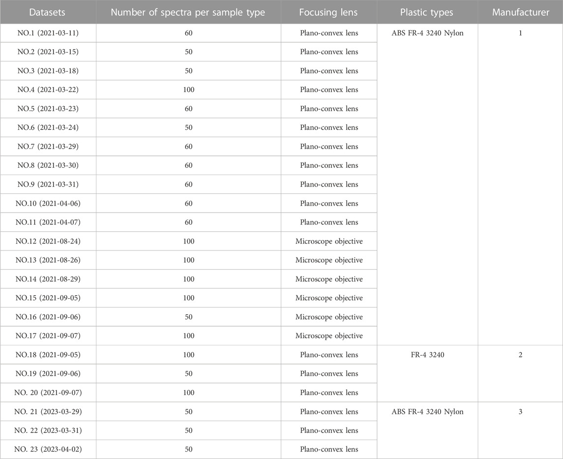
TABLE 2. Details about the make-up of the spectral datasets.
In general, the classification results of the model are affected by the fluctuation of the spectral data due to the variation factor between different measurements. To improve the performance of classification recognition models, spectral data preprocessing is implemented in four steps: baseline correction, spectral peak finding, correction of drift peaks, and total intensity normalization. The detailed processing is described in previous work (Li et al., 2017; Wang et al., 2018; Xu et al., 2020).
The impacts of noise and spurious peaks have been effectively removed from the preprocessed LIBS spectra, however, there are still redundant variables present in the characteristic spectral lines. To address this issue, variable selection identifies useful spectral variables to optimize the spectral differences between various samples and enhance the performance and interpretability of multivariate models. Typically, the choice of spectral variables can be made by employing a priori knowledge that is based on the structure and elemental makeup of a specific sample. However, because the plastic matrix is quite complicated, it is difficult to evaluate if the spectral emission lines of a particular element can accurately reflect the variations between samples. In this work, the Relief-F algorithm is utilized to carry out the process of feature selection and to calculate the important weights of the feature spectral lines. Relief-F is an extended version of the classical filtering feature selection method Relief (Cui et al., 2021), which evaluates the importance of variables by correlation.
Machine learning methods, a type of multivariate analysis methodology, can efficiently extract the implicit information from spectral data for qualitative analysis in LIBS. These methods establish the relationship between sample spectral data and corresponding category information to classify and identify unknown samples. Support vector machine (SVM) models are more commonly used in the data analysis and pattern recognition (Sattlecker et al., 2010; Sattlecker et al., 2011). For data that can be linearly separated, the SVM can perform discrimination directly in the original space. In cases where data is not linearly separable, SVM models use an appropriate kernel function to transform initial data into linearly separable data in a high-dimensional feature space.
The davis-bouldin index (DBI) is used to evaluate the effect of clustering (Davies and Bouldin, 1979). The DBI criterion is based on a ratio of within-cluster and between-cluster distances. DBI is defined as:
where Dij is the within-to-between cluster distance ratio for the ith and jth clusters.
In this research, multiple test scenarios were established to imitate the actual LIBS plastic sorting process, and the raw spectra collected under each scenario were distinct. Specifically, in scenario 1, spectral data collected on various dates were influenced by factors such as changes in laser, collection system, and lens-to-sample distance. Moreover, in scenario 2, in addition to the influence of the aforementioned factors, when the plano-convex lens is replaced with a microscopic objective for focusing, the focused spot diameter is reduced from ∅150 μm to ∅100 μm. As a result, both the sample ablation mass, as well as the power density at the focal point, are impacted. In Scenario 3, there are discrepancies in the manufacturing processes of plastic samples from various manufacturers, which results in more noticeable matrix effects. As a consequence, the LIBS spectra of samples produced by different manufacturers will be distinct from one another.
Based on these scenarios, three indicators are defined to assess the robustness of the classification model. First, the average correct classification rates (CCRs) of the model for spectra measured on different dates reflect the robustness over time (ROT). Second, the average CCRs of the model for spectra measured at different dates and with different focusing lenses is defined as the robustness over time and different focusing lenses (ROT & RFL). Lastly, the average CCRs of the model for spectra measured on different dates and using samples produced by different manufacturers was defined as robustness over time and different manufacturers (ROT & RDM). Here the correct classification rate (CCR) is calculated by the following equation.
where δi is the number of spectra classified correctly for each type of sample and q is the number of classes. N is the number of all samples.
Optimization of the model parameters is required to obtain the best classification accuracy. Table 3 lists the division of the dataset. Dataset NO.1 is used for model building in the training set. To obtain the optimal number of spectral features, datasets NO.2, NO.3, NO.4, and NO.5 are used in the validation set. The test set is used to verify the robustness of the model under different scenarios.
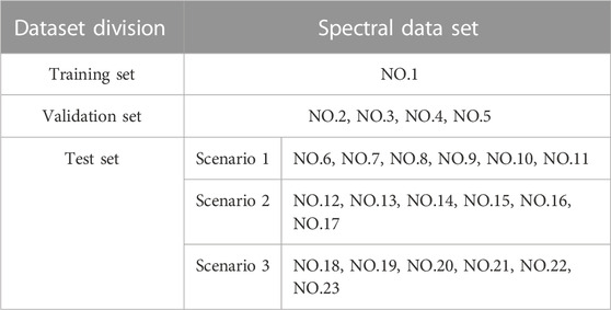
TABLE 3. Lists the division of the spectral data set.
Figure 2A shows the average LIBS spectra of the four plastics in data set NO.1. Although the four plastic samples belong to distinct species, it is clear from the figure that their LIBS spectral data contain about the same elemental information. The spectrum shows the non-metallic elements H (656.3 nm), O (777.3 nm), and N (744.6, 746.5, and 844.6 nm), as well as the CN molecular band (387.8 nm) and C2 molecular line (558.42 nm). Additionally, there are spectral lines for the metal elements Ca (393.4, 442.7, and 445.5 nm, etc.), Fe (315.4 nm and 317.5 nm), Mg (279.1 nm and 517.3 nm), Na (589.0 nm), and K (766.5 nm). Perhaps the presence of additives in the plastic materials caused the metallic lines to appear in the spectra. In addition, there are notable similarities among the LIBS spectral profiles of several plastic samples, such as the spectra of the 3240 and FR-4 samples. Although the constituent elements of the four plastic samples are similar, there are differences in the LIBS spectra. ABS displays a lower number of spectral lines compared to the other samples, and its Ca spectral line has a significantly lower intensity. Similarly, the spectral line intensities of Fe and Mg were weak in the Nylon samples.
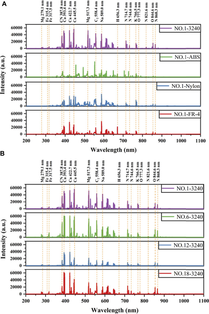
FIGURE 2. Comparison of the acquired LIBS spectra. (A) The average LIBS spectra of the four plastics in data set NO.1. (B) The spectra of the 3240 plastic sample collected under three different scenarios.
Figure 2B shows the spectra of the 3,240 plastic samples collected under three different scenarios. NO.1-3240 and NO.6-3240 are collected under scenario 1, which are extremely similar in their spectral profiles and differ mainly in the intensity of some characteristic spectral lines. When compared to the aforementioned datasets, NO.12-3240 exhibits a considerable intensity decrease of the spectral characteristic peak, which is due to the replacement of the plano-convex lens used for focusing during the experiment with a microscope objective. The maximum intensity of the characteristic peak is about 40,000. This is because, after focusing the microscope objective, the size of the laser spot decreases, resulting in a significant decrease in the size of the ablation crater and a reduction in the mass of the ablated plastic sample. For NO.18-3240 and NO.1-3240, in addition to the different collection dates, the plastic sample manufacturers are also different. The comparison of the two spectra sets revealed a difference in the intensity of several characteristic peaks, including stronger Ca 393.4 nm and Ca 422.7 nm in NO.18-3240, and stronger Mg 517.3, C2 558.4, and Na 589.0 nm in NO.1-3240. Meanwhile, the intensity ratios of the main characteristic spectral lines were calculated to make a clear comparison of the differences between the collected spectra in different scenarios. The calculated results are listed in Table 4, and there are significant differences in the intensity ratios of the characteristic spectral lines of the collected spectra under different scenarios, especially for Ca (393.4 nm)/Na (589.0 nm) and Ca (393.4 nm)/Mg (517.3 nm). There are significant differences in the acquisition spectra of the same plastic sample in different scenarios, which makes plastic classification and identification more challenging.
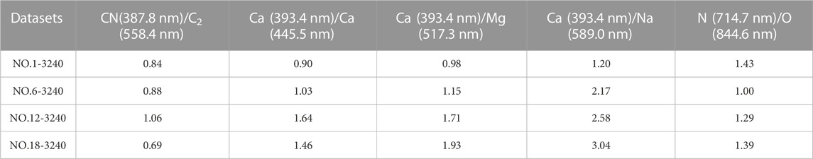
TABLE 4. Intensity ratios of the main characteristic spectral lines in the spectra of 3,240 samples collected under different scenarios.
In a further step, to quantitatively describe the discrepancy between the collected spectra in the three scenarios, the intensities of the spectra from different data sets were fitted, and lower fit coefficients indicated greater spectral discrepancy. The fitted curves between NO.1-3240 and NO.6-3240, NO.13-3240, and NO.18-3240 are depicted in Figures 3A–C, respectively. It is evident that differences occurred in the fitting coefficients for the spectra under different experimental conditions. The fitted curve in Figure 3A has a maximum fit coefficient of R2 = 0.938 because compared to other scenarios, only the date of spectral data acquisition has been changed. The R2 = 0.837 in Figure 3B, the fit coefficient that is noticeably lower than that in Figure 3A, is caused by a change in the sample’s ablation mass following the replacement of the focusing lens, which leads to a major variation in the spectra. In particular, the characteristic spectral lines of Ca at 422.7, 393.4, and 396.5 nm showed greater deviation from the fitted curve. Compared to Figure 3B, the fit coefficient of Figure 3C is further reduced (R2 = 0.823), and there are many data points in the plot that deviate significantly from the fitted curve. This could be as a result of the 3,240 samples’ varied additive composition from various manufacturers, which causes the matrix effects to be more evident. Fitting plots for the other three samples FR-4, ASB and Nylon were added to the support material as shown in Supplementary Figures S1–S3. The lower fit coefficients in different scenarios pose a higher challenge for plastic identification.

FIGURE 3. The fitted curves of spectral intensity between NO.1-3240 and NO.6-3240, NO.12-3240, and NO.18-3240.
In this research, the spectra of different types of plastic samples have similar spectral profiles, but there are discrepancies in the intensity of the characteristic spectral lines. Machine learning models can accomplish the classification task efficiently. LIBS combined with machine learning models can achieve accurate classification of spectra acquired under the same experimental conditions. However, changes in experimental conditions generally result in a decline in the classification recognition accuracy. Hence, the classification model should be robust enough to meet the testing requirements in under different experimental scenarios.
The original spectra were preprocessed using the method introduced in Section 2.4. This study considers the make-up of four different plastic types and the intensity of the characteristic spectral lines, and selects 85 spectral lines with intensities higher than 500 counts. The SVM classification model used the atomic and molecular spectral lines (C, CN, C2, H, N, O, Ca, Fe, K, Mg, Na, etc.) as input variables. The particle swarm optimization algorithm (PSO) in the training set combined with 10-fold cross validation was used to optimize the hyper-parameters of the SVM model. The spectra in the test set were preprocessed similar to the training set, and we compared the CCRs of the SVM model for the original and preprocessed spectra in Figure 4. It is clear from Figure 4 and Table 5 that there is a small improvement in the robustness of the model after spectral preprocessing. The ROT in Figure 4A increases from 58.4% for the original spectrum to 79.1% for the preprocessed spectrum. Similarly, the ROT&RFL increases from 65.54% to 75% in Figure 4B. Finally, ROT&RDM also increased from 65.5% to 67% in Figure 4C.
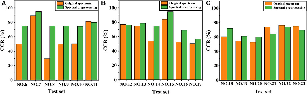
FIGURE 4. CCRs of the SVM model for the original and preprocessed spectra were tested separately. (A) Scenario 1, (B) Scenario 2, and (C) Scenario 3.
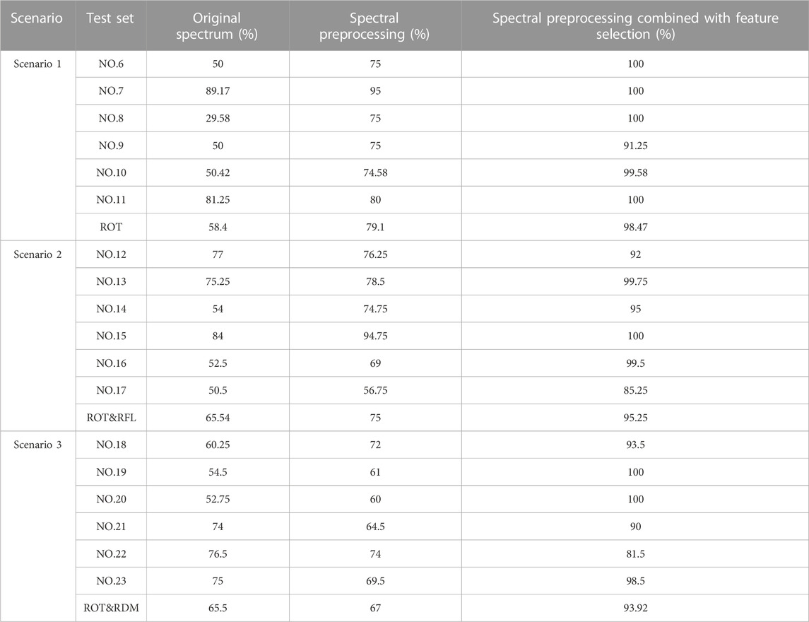
TABLE 5. CCRs predicted by the test sets under different methods.
Spectral preprocessing has three key advantages that enhance the SVM model’s robustness. Firstly, spectral preprocessing can effectively reduce the data dimensionality of the input variables and extract the spectral information. Moreover, the preprocessing can effectively reduce the RSD of the spectra, which means that the uncertainty of the spectra is reduced. Figure 5 shows the RSD of the original spectra of the main feature spectral lines in dataset NO.1 compared with the preprocessed spectra. For samples 3240, ABS, Nylon, and FR-4, the average RSDs of the characteristic spectral lines decreased from 10.85% to 8.49%, 19.26%–12.57%, 37.50%–22.14%, and 13.82%–11.01%, respectively. Particularly, the RSDs were decreased by more than half for the three characteristic spectral lines (Ca, N, and O) of Nylon samples. Moreover, spectral preprocessing reduces the DBI of spectral datasets. As shown in Table 6, the DBI decreased from 0.95 for the original spectra to 0.78 after preprocessing, which indicates that the preprocessing enhanced the clustering effect of the data.
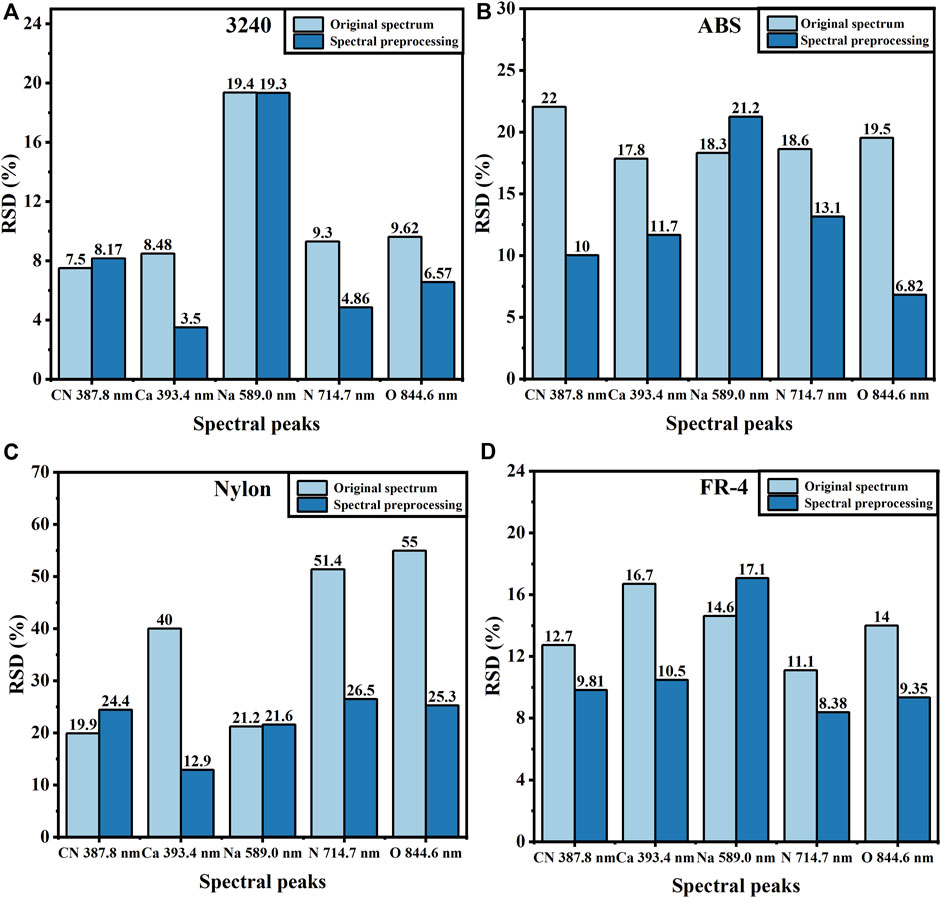
FIGURE 5. Comparison of the RSD between the original spectra and preprocessed spectra of the primary feature spectral lines in dataset NO.1. (A) 3240, (B) ABS, (C) Nylon, and (D) FR-4.
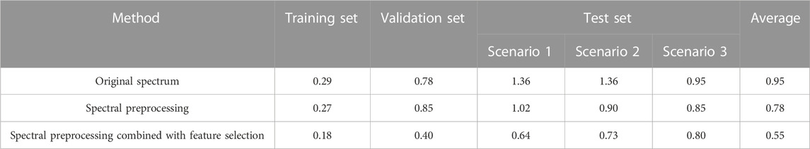
TABLE 6. Comparison of DBI under different methods.
Feature selection is essential in feature engineering and aims to find the optimal subset of features while excluding irrelevant or redundant ones. Feature selection can exclude irrelevant or redundant characteristics in order to minimize the amount of features, maximize spectral variance, enhance model accuracy, and decrease runtime. Typically, characteristic spectral emission lines are selected based on prior knowledge of sample structure and elemental composition. However, for plastic samples with a complicated matrix, it can be challenging to determine if a particular elemental spectral emission line is representative of the variations between samples. The present work utilizes the Relief-F algorithm to evaluate the spectral importance weights of the 85 feature spectral lines that were preprocessed in Section 3.2. Figure 6A depicts the relationship between the importance weights of the characteristic spectral lines and their wavelengths. Among them, the variables with greater importance weights are located at 420–450 nm (Cr and Ca elements) and 512–650 nm (Fe, C, and O elements and C2 molecular bands). After that, we ranked the spectral feature lines from greatest to smallest based on their importance weights, and the corresponding 85 feature selection models are trained in sequence. The feature selection models are applied to the validation set (NO. 2, 3, 4, and 5) to obtain the optimal number of feature spectral lines. As shown in Figure 6B, the average CCRs of the validation set varied with the input variables. When the first 19 most important feature variables are selected, the average CCR reaches a maximum of 92.6%.
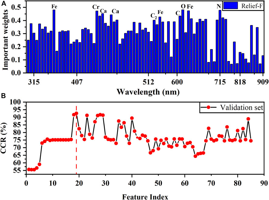
FIGURE 6. (A) Relief-F evaluates the important weights of the characteristic spectral lines. (B) The relationship between the mean CCRs of the validation set and the input variables.
We applied the optimized feature selection models obtained in the previous step to the test set. Figure 7 shows the CCRs that were predicted based on the spectra collected in different scenarios using different methods (original spectra, spectral preprocessing, and spectral preprocessing combined with feature selection). Our results, depicted in Figure 7 and Table 5, demonstrate a substantial enhancement in the SVM model’s robustness after feature selection. In Figure 7A, the ROT improves from 58.40% for the original spectrum and 79.10% for the spectral preprocessing to 98.47% for the feature selection. Similarly, in Figure 7B, ROT&RFL improves from 65.54% to 75%–95.25%. Finally, in Figure 7C, ROT&RDM also improved from 65.50% to 67%–93.92%.
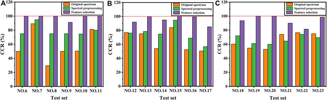
FIGURE 7. Predicted CCRs of original spectra, spectral preprocessing and feature selection methods for different scene acquisition spectra. (A) Scenario 1, (B) Scenario 2, and (C) Scenario 3.
Feature selection significantly improves the model’s robustness via three factors. First, the Relief-F algorithm, which evaluates the importance of variables by correlation, can maximize the spectral differences between different classes of samples. And the important features selected by the method are suitable for different application scenarios. Secondly, feature selection can significantly reduce the DBI of the dataset. As shown in Table 6, the average DBI is reduced from 0.95 for the original spectra and 0.78 for the spectral preprocessing to 0.55, which is 42.1% lower compared to the original spectra. The further reduction of DBI in comparison to preprocessed spectra indicates that feature selection can further improve the clustering performance of spectral datasets. Last but not least, feature selection considerably improves the similarity between the spectral variables of the test set and the training set. After 19 optimal features were selected, the fitting curves of the spectral variables are shown in Figure 8A–C, respectively. Comparing Figure 8A to Figure 3A, the R2 increases from 0.938 to 0.978, indicating that the similarity of spectral variables between scenario 1 and the training set has increased. Especially for Figure 8B and Figure 3B, R2 improves more significantly from 0.837 to 0.954. Similarly, for scenario 3, comparing Figure 3C with Figure 8C, R2 improves from 0.823 to 0.916.
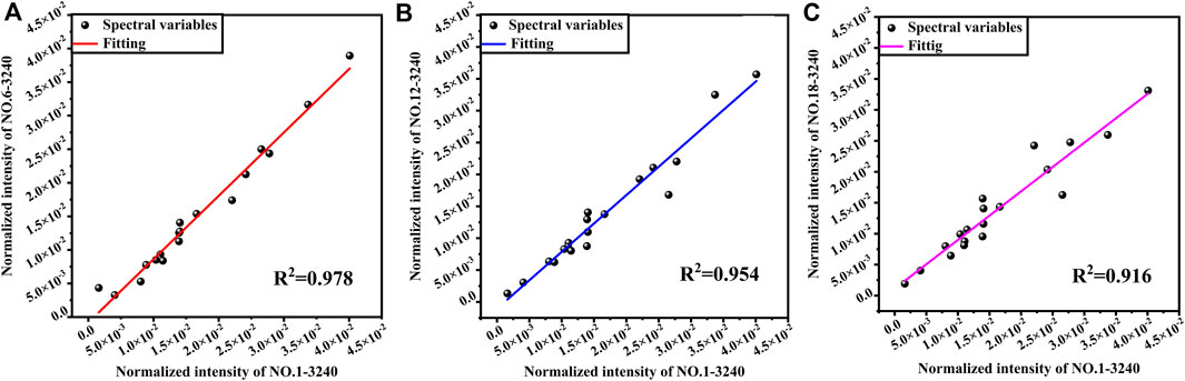
FIGURE 8. After selecting 19 optimal features, the curves between the spectral variables NO.1-3240 and NO.6-3240, NO.13-3240, and NO.18-3240 were fitted.
In this paper, spectral preprocessing combined with feature selection was used to improve the robustness of the SVM classification model for four typical plastic samples (ABS, nylon, 3240, and FR-4). LIBS spectroscopy measurements were taken under three distinct scenarios, including data collected at different dates, samples focused with different lenses, and the use of plastic samples from various manufacturers. We defined three indices (ROT, ROT&RFL, and ROT&RDM) to evaluate the robustness of the model. The feature importance of the preprocessed spectra was assessed using the Relief-F algorithm, and the maximum accuracy of the validation set is 92.6% when inputting the first 19 most important features. Further, the optimal model is applied to predict the test set. The ROT of the original spectrum, spectrum preprocessing, and spectral preprocessing combined with feature selection is 58.4%, 79.1%, 98.47%, respectively. Similarly, ROT&RFL of the three methods is 65.54%, 75%, and 95.25%, respectively. ROT&RDM is 65.5%, 67%, and 93.92%, respectively. Spectral preprocessing combined with feature selection effectively enhances the model’s robustness due to the following factors. 1) Spectral preprocessing can exclude the influence of noise on the model and significantly reduce the RSD of the spectrum. 2) Feature selection can enhance the spectral differences between different sample classes. 3) For the same class of samples, the similarity between the spectra of the test set and the training set is improved after feature selection. The results demonstrate that the combination of spectral preprocessing and feature selection can notably improve the robustness of the classification model, thereby proving the feasibility of the proposed plastic sorting and recycling method.
The raw data supporting the conclusion of this article will be made available by the authors, without undue reservation.
XX: Conceptualization, Methodology, Software, Data curation, Writing-original draft. GT: Methodology, Investigation. QW: Supervision, Funding acquisition. ZZ: Methodology, Investigation. KW: Validation. MB: Methodology, Investigation. YZ: Validation, Investigation. TL: Investigation. All authors contributed to the article and approved the submitted version.
This study was supported by National Natural Science Foundation of China (62075011).
The authors declare that the research was conducted in the absence of any commercial or financial relationships that could be construed as a potential conflict of interest.
All claims expressed in this article are solely those of the authors and do not necessarily represent those of their affiliated organizations, or those of the publisher, the editors and the reviewers. Any product that may be evaluated in this article, or claim that may be made by its manufacturer, is not guaranteed or endorsed by the publisher.
The Supplementary Material for this article can be found online at: https://www.frontiersin.org/articles/10.3389/fenvs.2023.1175392/full#supplementary-material
Adarsh, U. K., Kartha, V. B., Santhosh, C., and Unnikrishnan, V. K. (2022). Spectroscopy: A promising tool for plastic waste management. TrAC Trends Anal. Chem. 149, 116534. doi:10.1016/j.trac.2022.116534
Banaee, M., and Tavassoli, S. (2012). Discrimination of polymers by laser induced breakdown spectroscopy together with the DFA method. Polym. Test. 31, 759–764. doi:10.1016/j.polymertesting.2012.04.010
Chaqmaqchee, F. A. I., Baker, A. G., and Salih, N. F. (2017). Comparison of various plastics wastes using X-ray fluorescence. Am. J. Mater. Synthesis Process. 5, 24–27. doi:10.11648/j.ajmsp.20170202.12
Cui, X., Wang, Q., Kai, W., Geer, T., and Xu, X. (2021). Laser-induced breakdown spectroscopy for the classification of wood materials using machine learning methods combined with feature selection. Plasma Sci. Technol. 23, 055505. doi:10.1088/2058-6272/abf1ac
Davies, D. L., and Bouldin, D. W. (1979). A cluster separation measure. IEEE Trans. pattern analysis Mach. Intell., 224–227. doi:10.1109/tpami.1979.4766909
Dong, M., Lu, J., Yao, S., Li, J., Li, J., Zhong, Z., et al. (2011). Application of LIBS for direct determination of volatile matter content in coal. J. Anal. At. Spectrom. 26, 2183–2188. doi:10.1039/c1ja10109a
Fu, Y. T., Hou, Z. Y., Deguchi, Y., and Wang, Z. (2019). From big to strong: Growth of the asian laser-induced breakdown spectroscopy community. Plasma Sci. Technol. 21, 030101. doi:10.1088/2058-6272/aaf873
Global plastic production 1950-2021 (2022). Available at: https://www.statista.com/statistics/282732/global-production-of-plastics-since-1950/.
Hahn, D. W., and Omenetto, N. (2012). Laser-induced breakdown spectroscopy (LIBS), Part II: Review of instrumental and methodological approaches to material analysis and applications to different fields. Appl. Spectrosc. 66, 347–419. doi:10.1366/11-06574
He, Y., Wang, X., Guo, S., Li, A., Xu, X., Wazir, N., et al. (2019). Lithium ion detection in liquid with low detection limit by laser-induced breakdown spectroscopy. Appl. Opt. 58, 422–427. doi:10.1364/ao.58.000422
Labutin, T. A., Popov, A. M., Raikov, S. N., Zaytsev, S. M., Labutina, N. A., and Zorov, N. B. (2013). Determination of chlorine in concrete by laser-induced breakdown spectroscopy in air. J. Appl. Spectrosc. 80, 315–318. doi:10.1007/s10812-013-9766-8
Li, A., Guo, S., Wazir, N., Chai, K., Liang, L., Zhang, M., et al. (2017). Accuracy enhancement of laser induced breakdown spectra using permittivity and size optimized plasma confinement rings. Opt. Express 25, 27559–27569. doi:10.1364/oe.25.027559
Li, W., Lu, J., Dong, M., Lu, S., Yu, J., Li, S., et al. (2018). Quantitative analysis of calorific value of coal based on spectral preprocessing by laser-induced breakdown spectroscopy (LIBS). Energy & Fuels 32, 24–32. doi:10.1021/acs.energyfuels.7b01718
Liu, F., Ye, L. H., Peng, J. Y., Song, K. L., Shen, T. T., Zhang, C., et al. (2018). Fast detection of copper content in rice by laser-induced breakdown spectroscopy with uni- and multivariate analysis. Sensors 18, 705. doi:10.3390/s18030705
Liu, K., Tian, D., Deng, X., Wang, H., and Yang, G. (2019). Rapid classification of plastic bottles by laser-induced breakdown spectroscopy (LIBS) coupled with partial least squares discrimination analysis based on spectral windows (SW-PLS-DA). J. Anal. At. Spectrom. 34, 1665–1671. doi:10.1039/c9ja00105k
Neo, E. R. K., Yeo, Z., Low, J. S. C., Goodship, V., and Debattista, K. (2022). A review on chemometric techniques with infrared, Raman and laser-induced breakdown spectroscopy for sorting plastic waste in the recycling industry. Resour. Conservation Recycl. 180, 106217. doi:10.1016/j.resconrec.2022.106217
Patel, M., von Thienen, N., Jochem, E., and Worrell, E. (2000). Recycling of plastics in Germany. Resour. Conservation Recycl. 29, 65–90. doi:10.1016/s0921-3449(99)00058-0
Sattlecker, M., Baker, R., Stone, N., and Bessant, C. (2011). Support vector machine ensembles for breast cancer type prediction from mid-FTIR micro-calcification spectra. Chemom. Intelligent Laboratory Syst. 107, 363–370. doi:10.1016/j.chemolab.2011.05.007
Sattlecker, M., Bessant, C., Smith, J., and Stone, N. (2010). Investigation of support vector machines and Raman spectroscopy for lymph node diagnostics. Analyst 135, 895–901. doi:10.1039/b920229c
Shi, P. J., Wan, Y., Grandjean, A., Lee, J. M., and Tay, C. Y. (2021). Clarifying the in-situ cytotoxic potential of electronic waste plastics. Chemosphere 269, 128719. doi:10.1016/j.chemosphere.2020.128719
Vors, E., Tchepidjian, K., and Sirven, J. B. (2016). Evaluation and optimization of the robustness of a multivariate analysis methodology for identification of alloys by laser induced breakdown spectroscopy. Spectrochim. Acta Part B At. Spectrosc. 117, 16–22. doi:10.1016/j.sab.2015.12.004
Wang, Q., Cui, X., Teng, G., Zhao, Y., and Wei, K. (2020). Evaluation and improvement of model robustness for plastics samples classification by laser-induced breakdown spectroscopy. Opt. Laser Technol. 125, 106035. doi:10.1016/j.optlastec.2019.106035
Wang, Q. Q., Huang, Z. W., Liu, K., Li, W. J., and Yan, J. X. (2012). Classification of plastics with laser-induced breakdown spectroscopy based on principal component analysis and artificial neural network model. Spectrosc. Spectr. Analysis 32, 3179–3182.
Wang, X. S., Li, A., Wazir, N., Huang, S. Q., Guo, S., Liang, L., et al. (2018). Accuracy enhancement of laser induced breakdown spectroscopy by safely low-power discharge. Opt. Express 26, 13973–13984. doi:10.1364/oe.26.013973
Xia, J. J., Huang, Y., Li, Q. Q., Xiong, Y. M., and Min, S. G. (2021). Convolutional neural network with near-infrared spectroscopy for plastic discrimination. Environ. Chem. Lett. 19, 3547–3555. doi:10.1007/s10311-021-01240-9
Xu, X., Li, A., Wang, X., Ding, C., Qiu, S., He, Y., et al. (2020). The high-accuracy prediction of carbon content in semi-coke by laser-induced breakdown spectroscopy. J. Anal. At. Spectrom. 35, 984–992. doi:10.1039/c9ja00443b
Keywords: robustness of model, feature selection, spectral preprocessing, laser-induced breakdown spectroscopy, support vector machine
Citation: Xu X, Teng G, Wang Q, Zhao Z, Wei K, Bao M, Zheng Y and Luo T (2023) Spectral preprocessing combined with feature selection improve model robustness for plastics samples classification by LIBS. Front. Environ. Sci. 11:1175392. doi: 10.3389/fenvs.2023.1175392
Received: 27 February 2023; Accepted: 02 May 2023;
Published: 18 May 2023.
Edited by:
Changchun Huang, Nanjing Normal University, ChinaReviewed by:
Shunchun Yao, South China University of Technology, ChinaCopyright © 2023 Xu, Teng, Wang, Zhao, Wei, Bao, Zheng and Luo. This is an open-access article distributed under the terms of the Creative Commons Attribution License (CC BY). The use, distribution or reproduction in other forums is permitted, provided the original author(s) and the copyright owner(s) are credited and that the original publication in this journal is cited, in accordance with accepted academic practice. No use, distribution or reproduction is permitted which does not comply with these terms.
*Correspondence: Qianqian Wang, cXF3YW5nQGJpdC5lZHUuY24=; Geer Teng, Z2Vlci50ZW5nQGVuZy5veC5hYy51aw==
Disclaimer: All claims expressed in this article are solely those of the authors and do not necessarily represent those of their affiliated organizations, or those of the publisher, the editors and the reviewers. Any product that may be evaluated in this article or claim that may be made by its manufacturer is not guaranteed or endorsed by the publisher.
Research integrity at Frontiers
Learn more about the work of our research integrity team to safeguard the quality of each article we publish.