Seasonal prediction and possible causes of sudden losses of sea-ice in the Weddell Sea in recent years based on potential oceanic and atmospheric factors

The seasonal prediction of sea-ice concentration (SIC), especially sudden loss events, is always challenging. Weddell Sea SIC experienced two unprecedented decline events, falling from 2.21% in the austral winter of 2015 to 0.02% in the austral summer of 2016 and then falling to −2.32% in the austral spring of 2017. This study proposes several statistical prediction models for Weddell Sea SIC and performs them for a period that includes the sudden decline events. We identified six potential oceanic and atmospheric factors at different leading times that relate to the variability of the Weddell Sea SIC, including the Pacific Decadal Oscillation (PDO), Atlantic Multidecadal Oscillation (AMO), Niño12 sea surface temperature (SST), Southeastern Indian Ocean (SEIO) SST, Antarctic sea level pressure (SLP), and Weddell Sea surface air temperature (SAT). Multiple linear regression models were employed to establish equations to simulate the variation of Weddell Sea SIC under three groups of climate factors for 1979–2012. These models could effectively reproduce the low-frequency variation of SIC in the Weddell Sea during the simulation period and the high-frequency values through two kinds of error-correction methods developed in this study. After applying these error correction methods, the correlation coefficients (absolute errors) of these models were enhanced (decreased) during the simulation period. In the prediction period of 2013–2018, the corrected models generally predicted well the sudden losses of Weddell Sea SIC. The possible primary factors influencing these sudden losses were the PDO, Niño12 SST, Southern Annular Mode (SAM), and SAT during 2015–2016 and the AMO, PDO, Niño12 SST, SAM, and SAT during 2016–2017.

1 Introduction

The Antarctic, one of the planet’s main heat sinks, retains a crucial place in both the southern hemisphere and the overall climate system (Mayewski et al., 2009), having profound effects on atmospheric and oceanic circulation and global energy transport (King and Turner, 1997). Antarctica is covered in ice all year round and is surrounded by sea-ice, which has great potential to contribute to climate variability and change (Bintanja et al., 2013) and exhibits strong interannual variability due to the absence of encircling land (King and Turner, 1997). Sea ice plays a variety of roles in processes involving radiation, energy, and mass transfer, including changing the upper ocean’s albedo, obstructing the exchange of heat and water vapor between the ocean and atmosphere (Turner et al., 2017), changing ocean salinity, and influencing the Antarctic bottom waters due to global ocean circulation (Ohshima et al., 2013; Kitade et al., 2014; Haumann et al., 2016). It can affect the climate system on various time scales. Moreover, sea-ice is a crucial component of the Antarctic ecosystem, providing a habitat for seals, penguins, and krill (Meyer et al., 2017; Jenouvrier et al., 2021) and is essential to the continent’s biogeochemical processes.

Since the first satellite observations in 1979, quantitative descriptions and understanding of sea-ice variability have emerged. In contrast to the rapid decline of sea-ice in the Arctic (Serreze and Stroeve, 2015), Antarctic sea-ice extent (SIE) had been on a slow but significant upward trend with remarkable regionality (Parkinson and DiGirolamo, 2016; Comiso et al., 2017). The Antarctic SIE continued to set new records for the highest value in September 2012–2014, reaching 12.8 million km² (Turner et al., 2015), which ran counter to the concept that sea-ice will melt under a global warming scenario; its failure to do so is known as the “Antarctic paradox” (King, 2014). However, there has been a noticeable change in recent years. The Antarctic SIE of nearly all oceans reduced, reaching a minimum record of 2.07 million km² in 2017 (Turner and Comiso, 2017; Schlosser et al., 2018). The SIE in the Weddell Sea has the greatest decline, with a loss of 1 million km² since 2013. Nevertheless, this decline was absent from several areas of the western Ross Sea and the Indian Ocean (Parkinson, 2019; Eayrs et al., 2021). Thereafter, the Antarctic SIE slowly rebounded (Li et al., 2021).

There have been numerous studies on the origins of the recent decline of Antarctic sea-ice. In terms of atmospheric circulation, the northerly wind anomaly induced by pre-austral spring zonal wave 3 (ZW3) provided a precondition for sea-ice reduction in the summer of 2016 (Schlosser et al., 2018; Wang et al., 2019), which has also been confirmed in simulation experiments (Kusahara et al., 2018). The weakening ZW3 and Southern Annular Mode (SAM) in negative phase together led to sea-ice reduction, which was associated with the downward transmission of the Madden–Julian Oscillation (MJO) and stratospheric polar vortex anomaly signals (Seo and Son, 2012; Kidston et al., 2015). Frequent cyclone activity was another reason for the decrease in Weddell Sea sea-ice (Jones and Simmonds, 1993; Turner et al., 2020). In terms of the ocean, the El Niño–Southern Oscillation (ENSO) can usually influence the variability of Antarctic sea-ice through atmospheric bridges like the Pacific South American (PSA) pattern (Mo and Paegle, 2001; Kwok and Comiso, 2002; Stuecker et al., 2015; Stuecker et al., 2017). However, the relationship between ENSO and Antarctic sea-ice weakened after 2002 (Dou and Zhang, 2022), and experiments with actual sea surface temperature (SST) anomalies forcing flat ocean coupled models suggested that the contribution of El Niño was not significant (Purich and England, 2019); thus, the contribution from ENSO to sea-ice loss would require additional model validations. The tropical Indian Ocean played a more important role than the Pacific Ocean, and a strong negative phase of the Indian Ocean Dipole (IOD) occurring in the spring of 2016 inspired a ZW3-like circulation anomaly (Meehl et al., 2019; Purich and England, 2019; Wang et al., 2019). In addition, the warm spring polar ocean was also conducive to sea-ice reduction (Lecomte et al., 2017; Meehl et al., 2019). The occurrence of large interglacial lakes in summer was an important cause of sea-ice reduction in the Weddell Sea (Swart et al., 2018; Turner et al., 2020).

Numerical model simulations are also useful methods for enhancing our understanding of sea-ice. Its interaction with the ocean and atmosphere provides the physical basis for simulating and predicting sea-ice variation. The predictability of Arctic sea-ice on various time scales in different seasons has been extensively explored (Guemas et al., 2016; Mohammadi-Aragh et al., 2018; Cruz-García et al., 2019). In addition, statistical models have been used to predict sea-ice variation. Wang et al. (2018) compared the weekly prediction effects of the Markov chain model and vector autoregressive model on sea-ice in the Arctic. Yuan et al. (2016) established the Markov chain model at a seasonal to intra-seasonal scale. Machine learning, particularly deep learning, has also been recently used to predict sea-ice variation to tackle non-linear interaction issues (Kim et al., 2020; Liu et al., 2021a). Liu et al. (2021b) trained convolutional long short-term memory (ConvLSTM) networks to predict SIC at weather to sub-seasonal scales in the Barents Sea. Whereas the prediction of Antarctic sea-ice has only recently received widespread international attention, it has received relatively little research. Chen and Yuan (2004) built Markov chain models to provide one of the first explorations of seasonal predictions of sea-ice variation in the Antarctic. Holland et al. (2013) evaluated the initial-value predictability of Antarctic sea-ice in the Community Climate System Model 3. Coupled climate models are also major tools for simulating sea-ice evolution. Hosking et al. (2013) used the CMIP5 model to conduct a preliminary assessment of SIE prediction. Polvani and Smith (2013) used this model to demonstrate how natural variability contributes to Antarctic sea-ice change more than anthropogenic factors. Shu et al. (2020) employed CMIP5 and CMIP6 models to reproduce the seasonal changes of SIE, although their simulation ability was limited.

The loss of the Weddell Sea SIC was the largest contributor to total Antarctic sea-ice reduction since 2015, accounting for 34%, with the negative anomaly continuing until 2020. This study aims to investigate the variation of Weddell Sea SIC and the following questions. Are the atmospheric and oceanic factors prior to the variation of Weddell Sea SIC? Can the models established by those potential predictors simulate the variation of Weddell Sea SIC during past decades? Can those seasonal prediction models predict the sudden decrease of Weddell Sea SIC in recent years? Which potential predictors are the main contributing factors to the sudden decrease of Weddell Sea SIC? With these questions in mind, we identified six potential influence factors of the variation of Weddell Sea SIC, established three seasonal prediction models of Weddell Sea SIC according to multiple linear regression equations, performed prediction during the period 2013–2018, and explored the main contributions and influences of factors in the decline of Weddell Sea SIC. The paper is organized as follows: the methods and datasets are described in Section 2. The declines of SIC in the Weddell Sea are shown in Section 3. The potential oceanic and atmospheric predictors are identified in Section 4. Three seasonal prediction models are established in Section 5, and two error correction methods are developed in Section 6. The predictions of sudden losses of Weddell Sea SIC are shown in Section 7. The possible causes of recent sudden losses of Weddell Sea SIC are revealed in Section 8, and summary and discussion are given in Section 9.

2 Data and methods

2.1 Data

Four types of datasets and three indices were used in this study. The sea-ice data were obtained from the National Snow and Ice Data Center (NSIDC), which provided a Climate Data Record (CDR) of sea-ice concentration from Passive Microwave Data version 3 (Peng et al., 2013; Meier et al., 2017). This work only focused on the southern hemisphere and built 168 seasonal samples based on monthly merged SIC datasets from 1978 to 2020 on a 25 km × 25 km grid (https://nsidc.org/data/g02202/versions/3).

The second dataset was the monthly median Hadley Centre Sea Ice and Sea Surface Temperature data set (HadISST) from the Met Office Marine Data Bank with 1 × 1° resolution from 1975 to 2018 (Rayner, 2003) (https://www.metoffice.gov.uk/hadobs/hadisst). In addition, this study used a Hadley Centre and the fifth Climatic Research Unit at the University of East Anglia temperature (HadCRUT5) gridded dataset of global historical surface air temperature (SAT) monthly anomalies relative to the reference period of 1961–1990 (Morice et al., 2021). The dataset was on a 5° grid from 1975 to 2018 and was a collaborative production of the Met Office Hadley Centre and the Climatic Research Unit at the University of East Anglia (https://www.metoffice.gov.uk/hadobs/hadcrut5).

The fourth dataset was the fifth-generation ECMWF reanalysis (ERA5) mean sea level pressure (SLP) dataset produced by the European Centre for Medium-Range Weather Forecasts (ECMWF) (Hersbach et al., 2020). We took monthly data from the 1975–2018 range on a 1 × 1° grid (https://cds.climate.copernicus.eu).

We also used the Pacific Decadal Oscillation (PDO) index, Atlantic Multidecadal Oscillation (AMO) index, and Niño12 SST index for 1975–2018. The PDO is defined as the leading mode of monthly SST anomalies in the North Pacific poleward of 20°N (Mantua et al., 1997). Its positive (negative) phase manifests positive (negative) SST anomalies in the eastern North Pacific and negative (positive) SST anomalies in the central and western North Pacific. The AMO is identified as the large-scale multidecadal fluctuations of the detrend low-pass filtered average SST anomalies in the North Atlantic Ocean typically over 0–80°N (Enfield et al., 2001). The Niño12 SST index is also one of the indices used to monitor SST anomalies averaged across a given region in the tropical Pacific. It usually represents El Niño conditions in coastal South America (0–10°S, 80°–90°W).

This paper employed the austral seasonal mean variables averaged from monthly data and divided per year into austral spring (previous September–October–November, SON), summer (previous December–current January–February, DJF), autumn (current March–April–May, MAM), and winter (current June–July–August, JJA). The analyses of this paper were based on the austral seasons.

2.2 Method

Multiple linear regression refers to a statistical technique that is used to predict the outcome of a variable based on the value of two or more variables (Xiao et al., 2021). Linear regression attempts to establish the relationship between the variables along a straight line. This study used a multiple linear regression model to simulate and predict the SIC anomaly in the Weddell Sea. The multiple linear regression equation is as follows.

$\begin{array}{c}\stackrel{\sim }{Y}=b_0+b_1{X}_1+b_2{X}_2+\cdots +b_p{X}_{p,}\end{array}(1)$

where $\stackrel{\sim }{Y}$ is the predicted value of the dependent variable, b₀ is the intercept, X₁ through X_p are independent variables or predictors, b₁ through b_p are the regression coefficients for X₁ through X_p, and respectively represent the change in Y relative to a one-unit change in X. The significance of the equation can be judged by the magnitude of the variance test or the complex correlation coefficient. If significant, the equation is considered statistically significant, and the independent variable X has an effect on the dependent variable Y. A t-test is used to check the significance of individual regression coefficients.

In addition, the jackknife method (Efron, 1979) was used to check the stability of the prediction model. The jackknife is based on the following steps. During the fitting period, the entire time series excludes one group of data at a time, and the regression model is rebuilt with the remaining data. The statistical indicators such as the complex correlation coefficient (R²), the coefficient of complex determination after adjustment for degrees of freedom (R_adj²), the F-test value, and the significance level (p-value) are calculated (Huang, 2004). Then, a group of data is excluded year by year, and the aforementioned steps are repeated to obtain multiple sets of statistical indicators. If the statistical indicators are close to the results of the original regression model, including all years of the fitting period, and the range of variation is minimal, the regression model is stable and reliable (Liu et al., 2013).

The significance tests of the correlation coefficient in this work were all calculated based on the effective degrees of freedom (Pyper and Peterman, 1998).

$\begin{array}{c}{N}_{eff}\approx \frac{N}{1+2{\displaystyle \sum }_{k=1}^N\frac{N-k}{N}{r}_1\left(k\right)r_2\left(k\right)},\end{array}(2)$

where N is the number of samples and k represents the time lag value. r₁ and r₂ are the autocorrelation coefficient with lagging k of two sequences. If not stated, all two-sided t-tests in this study were based on the effective degrees of freedom.

This study evaluated the model performance by following three accuracy metrics: the anomaly correlation coefficient (ACC), root-mean-square error (RMSE), and mean absolute error (MAE). The ACC is a skill score metric to assess the similarity quality of the prediction model, and its value is between −1 and 1. The RMSE is used to measure the deviation of the predicted value from the observed value. The MAE can accurately depict the actual situation of the prediction error (Kim et al., 2020). The calculation formulas are as follows.

$\begin{array}{c}ACC=\frac{\sum \left(predictedSIC-\overline{predictedSIC}\right)\left(observedSIC-\overline{observedSIC}\right)}{\sqrt{\sum {\left(predictedSIC-\overline{predictedSIC}\right)}^2}\sqrt{\sum {\left(observedSIC-\overline{observedSIC}\right)}^2.}}\end{array}(3)$

$\begin{array}{c}RMSE=\sqrt{\frac{1}{N}{\displaystyle \sum }_{i=1}^N{\left(predicted{SIC}_i-observed{SIC}_i\right)}^2}.\end{array}(4)$

$\begin{array}{c}MAE=\frac{1}{N}{\displaystyle \sum }_{i=1}^N\left|predicted{SIC}_i-observed{SIC}_i\right|\end{array}.(5)$

3 Declines of Weddell Sea SIC in recent years

The trend of Antarctic SIC from 2014 to 2020 is shown in Figure 1. It can be seen that the most significant fall was on the eastern edge of multi-year ice in the western and in southeast corner of the Weddell Sea, where the downward trend in most areas surpassed 0.006% per season, and the maximal domain significantly exceeded 0.012% per season. Other regions with declining tendencies were along the outer edge of East Antarctica and in the northern Bellingshausen and Amundsen Seas. While increased SIC was located in the southern Bellingshausen and Amundsen Seas and part of the Indian Ocean near Antarctica, the increasing trends in all regions failed to pass the significance test. Therefore, we focused on the changes of SIC over the Weddell Sea and chose the region of 60°–80°S and 60°W–0° as the research domain in this study.

FIGURE 1

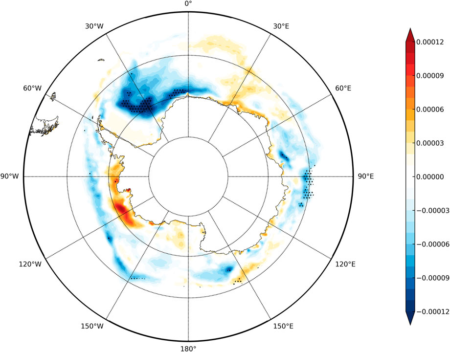
FIGURE 1. Trend of Antarctic SIC during 2014–2020 (unit: % per season). The bold dots denote statistically significant change at 95% confidence level.

As shown in Figure 2, the time series of Weddell Sea SIC had risen insignificantly throughout the past four decades. SIC in the Weddell Sea declined in the 1980s and increased until the mid-1990s and then underwent another temporary fall for about 5 years. At the beginning of the 21st century, it began to gradually increase again and reached a record-breaking peak value of 2.42% in 2014. However, there were two significant sharp declines of the Weddell Sea SIC anomaly after 2014, as the anomaly dropped from 2.21% in the austral winter of 2015% to 0.02% in the austral summer of 2016 and from 0.42% in the austral autumn of 2016% to −2.32% the next spring. The positive anomaly first dropped close to zero and then dropped to a negative value, reaching the lowest on record for SIC in the Weddell Sea before rebounding after 2018. It had recovered to positive by 2020. SIC in the Weddell Sea had significant periods of one to two decades based on the wavelet analysis (not shown), which were similar to that of PDO. Therefore, we suspected that the PDO and even the global ocean might be potential factors affecting the change of sea-ice. In other words, Weddell Sea SIC experienced an unprecedented reduction from 2015 to 2018 and contributed the most in the following overall significant decline in Antarctic sea-ice in the spring of 2016 (Turner et al., 2017). Therefore, the variation of the Weddell Sea SIC is the key to understanding the variation of Antarctic SIC.

FIGURE 2

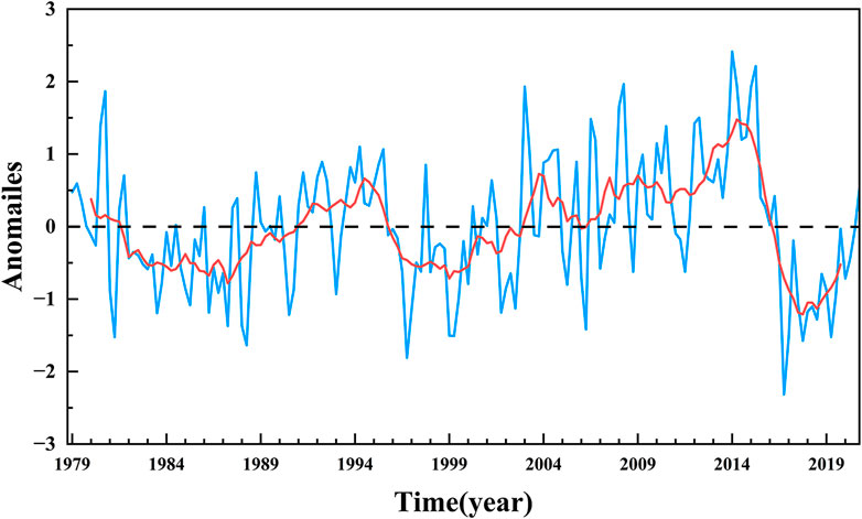
FIGURE 2. Time series of Weddell Sea averaged SIC anomaly 1979–2020 (unit: %). The blue line represents the averaged seasonal anomaly, and the red line denotes the nine-season running average of the SIC anomaly.

The spatial evolution of the SIC anomaly in the Weddell Sea in the austral summer from 2015 to 2018 is shown in Figure 3. The SIC anomaly in the summer of 2015 was positive, exceeding 0.3% mainly in the northwest and southeast Weddell Sea (Figure 3A). There was no discernible changing trend in the western multi-year ice region. The SIC anomaly thence decreased in 2016. Only the northeastern and southeastern parts of the Weddell Sea still exhibited positive anomalies, but the extent was much reduced (Figure 3B). The SIC anomaly in the northwestern Weddell Sea was negative but was only around 0.15%. The SIC anomaly in the eastern boundary of the multi-year ice in the western Weddell Sea remained positive in the summer of 2017. After the second dip, the SIC anomaly in the other regions was negative, except in the western Weddell Sea; those in the northwest and southeast reached −0.3% (Figure 3C). Thereafter, the SIC anomaly began to recover and increased at a slower rate; the positive anomaly center was more than 0.25% in the northwest, but the negative anomalies still remained in the large area of the east, while the largest anomaly was observed in the southeast in 2018 (Figure 3D).

FIGURE 3

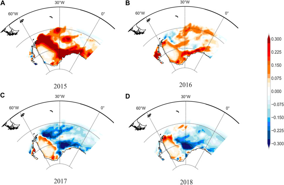
FIGURE 3. Anomaly of Weddell Sea SIC in austral summer of 2015 (A), 2016 (B), 2017 (C), and 2018 (D) based on the climatology of 1979–2020 (unit: %).

4 Potential oceanic and atmospheric predictors

We calculated the Pearson correlation coefficients between the SST, SLP, and SAT variables at different leading times and Weddell Sea SIC and selected the correlation maps shown in Figure 4 with maximal significant grids. The significant correlation between Weddell Sea SIC and ten-season ahead SST was mainly distributed in the 20°N poleward of the Pacific Ocean, showing negative correlations along the western coast of North America and positive correlations in the region from the Sea of Japan to the central North Pacific. This pattern was similar to that of the PDO negative phase. There were also insignificant positive and significant negative correlations in the South Pacific and East Pacific, respectively. The distribution of correlation in the Pacific Ocean seemingly assembled the negative phase of the Interdecadal Pacific Oscillation (IPO). We also calculated the correlation coefficients between the Weddell Sea SIC and simultaneous and ten-season leading IPO, respectively. The former was insignificant while the latter was less than with PDO. In addition, the correlation between SST in the South Pacific Ocean and the mid-East Pacific Ocean and the Weddell Sea SIC was insignificant (Figure 4A). Therefore, the PDO (IPO) was (not) identified as a potential predictor of Weddell Sea SIC. The convective heating anomalies caused by the SST anomaly in the Pacific Ocean have contributed to the Amundsen Sea Low and the development of sea-ice through the abnormal Rossby wave response (Meehl et al., 2016). There were also significantly negative correlations along the western coast of northern South America, with the maximal value exceeding 0.25 (Figure 4B). This region (82°–98°W, 10°–18°S) was quite close to the Niño12 region, so we calculated the correlation coefficient between them with the 168 samples. It was 0.79 and indicated their intimate relationship. Accordingly, we selected the SST anomaly in this area as a new index as the deputy of the well-known Niño12 SST, which can represent the role of ENSO to some extent. On one hand, ENSO can excite an anomalous Rossby wave response in the mid-high latitudes of the southern hemisphere to affect the intensity of the Amundsen Sea Low. The resulting meridian anomaly in the southern hemisphere can influence the dynamic transport and the heat flux between atmosphere and ocean, thus changing the distribution of sea-ice in the Antarctic (Liu et al., 2002; Purich and England, 2019). On the other hand, ENSO can also influence Antarctic sea-ice by affecting the Peruvian cold current and other ocean processes. In the Indian Ocean, there was a significantly positive correlation in the southeastern Indian Ocean and to the south of Australia (Figure 4C). Since the Indian Ocean Dipole (IOD) has contributed to the decline of sea-ice in Antarctic (Wang et al., 2019), we also calculated the correlation between Weddell Sea SIC and the IOD mode index (Saji et al., 1999), which was not significant. Therefore, the SST anomaly in this area (110°–140°E, 35°–45°S) was considered a potential influencing factor and defined as the Southeastern Indian Ocean (SEIO) SST. The tropical convection over the Indian Ocean can excite the abnormal Rossby wave following the waveguide of the high-latitude westerly jet eastward across the Southern Ocean. The Rossby wave contributes to increased cyclone–anticyclone anomalies in the southwestern and southeastern South America and the ZW3 anomaly pattern and thus changes the variability of sea-ice (Wang et al., 2019). Furthermore, Weddell Sea SIC was closely related to North Atlantic SST. There were positive correlations in the northern and tropical North Atlantic Ocean, with significant maximal correlation in the former exceeding 0.3 and insignificant correlation in the latter (Figure 4D). Such spatial patterns of correlation in the Atlantic Ocean were similar to those of AMO. Xiao et al. (2014) chose the SST anomaly in the northernmost and southernmost parts of the North Atlantic Ocean as a new index, which was highly correlated with the AMO index; this new index essentially represented the variation of the AMO. Therefore, the sum of half of the SST anomalies in these two regions (55°–15°W, 50°–62°N and 50°–20°W, 5°–20°N) was defined as a new index to represent the AMO variation in this study. The warming SST associated with the AMO can reduce the surface level pressure of the Amundsen Sea Low and result in the redistribution of dipole-like sea-ice between the Ross Sea and the Amundsen–Bellingshausen–Weddell Sea and the warmer Antarctic Peninsula (Li et al., 2014). In summary, according to the analysis of global SST anomalies, the PDO, AMO, Niño12, and SEIO SSTs, associated with the Weddell Sea SIC variation, were identified as potential oceanic predictors of Weddell Sea SIC.

FIGURE 4

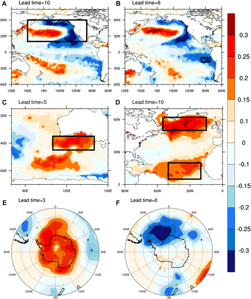
FIGURE 4. Correlation coefficients between Weddell Sea SIC and SST (A–D), SLP (E) and SAT (F) at different leading times. The leading times are indicated on the left of each panel. The key oceanic regions related to the Weddell Sea SIC shown in the black boxes. The stippling in all the panels denotes the 95% confidence level based on the two-sided student t-test.

In addition, we also took into account the contribution of atmospheric predictors from the relationship between SLP and Weddell Sea SIC. There was a positive correlation around Antarctica (Figure 4E), indicating that Weddell Sea SIC tended to increase when SLP in Antarctica was positive. The Southern Annular Mode is the zonal pressure difference between the 40°S and 65°S latitudes, and its negative phase corresponds to higher SLP anomalies over the Antarctic and lower ones along the belt of 30°–50°S latitude (Nan and Li, 2003). The correlation pattern in Figure 4E assembled the negative phase of SAM, especially in high latitudes. The correlation between Antarctic SLP (65°–85°S) and the SAM index was −0.82, exceeding the 99.9% confidence level, suggesting that the Antarctic SLP anomaly could represent the variation of the negative SAM index. The correlation coefficient between the SAM index at the three-season leading time and Weddell Sea SIC was −0.14, which was smaller than that between SLP and SIC of 0.24. Therefore, we used the negative Antarctic SLP anomaly to represent the SAM index in this study, and we considered the new SAM index as a potential influencing factor of Weddell Sea SIC. The negative phase of SAM can weaken the near-surface circumpolar west wind and produce a positive wind stress curl and southward Ekman transport. The warmer surface water is transported south and results in increased SST (Meehl et al., 2019). There was significant negative correlation between SIC and the simultaneous SAT over the Weddell Sea, which indicated that the higher the SAT, the less Weddell Sea SIC there is (Figure 4F). The simultaneous Weddell Sea SAT cannot be used as a predictor of Weddell Sea SIC. If the reliable Weddell Sea SAT is used a dependent variable in the prediction model of Weddell Sea SIC, it is helpful to learn the maximal improvement of the prediction model under the situation of a perfect prediction of Weddell Sea SAT. Consequently, the Weddell Sea SAT was considered a simultaneous influencing factor of Weddell Sea SIC. The increased air temperature inhibits the development of sea-ice. Therefore, we identified the PDO, AMO, Nino12 and SEIO SSTs, SAM, and SAT as potential predictors of Weddell Sea SIC.

Figure 5 depicts the leading–lagged correlation coefficients between Weddell Sea SIC and the aforementioned six potential predictors. It was found that both SEIO and Niño12 SSTs led the changes of Weddell Sea SIC by five seasons, AMO by eleven, PDO by ten, and SAM by three seasons—all of which had passed a two-sided t-test with the 95% confidence level. The most significant correlation coefficient was between SAT and SIC in the same period. The influence of ocean factors (such as PDO, AMO, SEIO, and Niño12 SSTs) on Weddell Sea SIC was ahead of these of atmospheric factors for at least more than 1 year. This might be explained by the ocean’s slow motion and long-term memory compared to relatively quick atmospheric changes. Only the atmosphere above Antarctica and the global oceans in both the northern and southern hemisphere potentially influenced the variation of the Weddell Sea SIC. The leading times of the ocean variables in the southern hemisphere (Niño12 and SEIO SSTs) were five seasons, which were shorter than the leading times of the ocean factors in the northern hemisphere (PDO and AMO) of ten seasons. The relationships between oceanic and atmospheric factors at different leading times and Weddell Sea SIC were significant. These leading oceanic and atmospheric factors could be used to predict the variability of Weddell Sea SIC in advance.

FIGURE 5

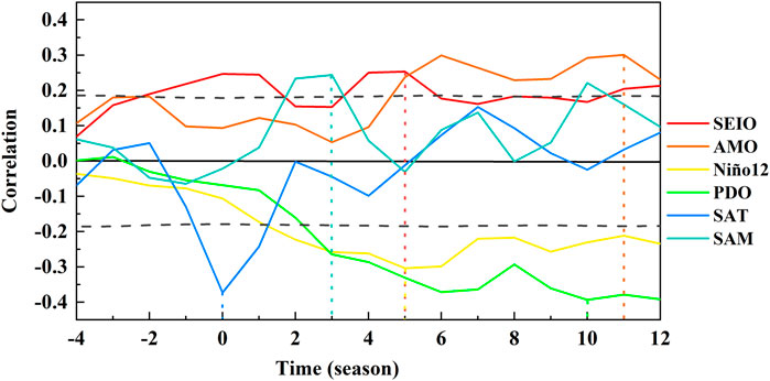
FIGURE 5. Leading–lagged correlation coefficients between Weddell Sea SIC and various climate predictors listed on the right of the panel. Positive abscissa value indicates that the predictor is ahead of Weddell Sea SIC, and negative value indicates that the factor lags behind Weddell Sea SIC. The maximum correlation is identified by a vertical line of corresponding color. The black dashed lines denote correlation coefficients passed the two-sided t-test with the 95% confidence level using the effective degrees of freedom.

5 Establishing seasonal prediction models

This section employed the aforementioned six factors at individual leading times to establish the seasonal prediction equations of Weddell Sea SIC based on the multiple linear regression models. We first used data sets in the fitting period 1979–2012 to build models to simulate variations of Weddell Sea SIC and then examined the performance of the model during the predicting period 2013–2018.

In order to explore the contributions of atmospheric and oceanic predictors to changes in the Weddell Sea SIC, we divided the aforementioned six predictors into three groups (Table 1 to explore the independent influence of the oceanic factors (including the PDO, AMO, SEIO, and Niño12 SSTs), the combined effects of the aforementioned oceanic factors and SAM, and the joint effects of oceanic factors, SAM, and Weddell Sea SAT. The third group of potential influencing factors (including the leading PDO, AMO, SAM, SEIO, and Niño12 SSTs and simultaneous Weddell Sea SAT) can help us understand the best simulation we can achieve with the precise prediction of Weddell Sea SAT. According to the three groups of potential influencing factors, three equations were established based on the multiple linear regression models:

$\begin{array}{c}{\stackrel{\sim }{SIC}}_i=0.05-0.05\ast {PDO}_{i-10}-0.22\ast {Ni\stackrel{\sim }{n}o12}_{i-5}\\ +0.16\ast {SEIO}_{i-5}+0.07\ast {AMO}_{i-11}.\end{array}(6)$

$\begin{array}{c}{\stackrel{\sim }{SIC}}_i=0.03-0.03\ast {PDO}_{i-10}-0.20\ast {Ni\stackrel{\sim }{n}o12}_{i-5}+0.17\ast {SEIO}_{i-5}\\ +0.07\ast {AMO}_{i-11}+0.20\ast {SAM}_{i-3}.\end{array}(7)$

$\begin{array}{c}{\stackrel{\sim }{SIC}}_i=0.02-0.06\ast {PDO}_{i-10}-0.17\ast {Ni\stackrel{\sim }{n}o12}_{i-5}+0.21\ast {SEIO}_{i-5}\\ +0.08\ast {AMO}_{i-11}+0.24\ast {SAM}_{i-3}-0.31\ast {SAT}_i.\end{array}(8)$

TABLE 1

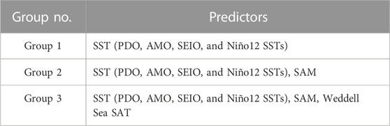
TABLE 1. Three groups of six predictors for the seasonal prediction models.

These prediction models aimed to investigate the contribution of only leading oceanic factors (Eq. (6)), joint contributions of leading oceanic factors and SAM (Eq. 7), joint contributions of leading oceanic factors, SAM, and a perfect prediction of simultaneous Weddell Sea SAT (Eq. 8) to the variations in Weddell Sea SIC. The R_adj² of the three models were respectively 0.117, 0.177, and 0.319. All these prediction models were credible and reasonable because they were statistically significant after F-testing at the 99.9% confidence level. Furthermore, the stabilities of Eqs (6)–(8) were examined by the jackknife method, with the results of Eq. (8) shown in Table 2. The R² of the equation with all predictors was 0.349, the R_adj² was 0.319, and the F-test value was 11.537, which passed the significance test at the 99.9% confidence level (p < 0.001). The average R², R_adj², and F-test value by jackknife were, respectively, 0.349, 0.319, and 11.461: close to the original values of Eq. (8). The relative deviation of the average R² by the jackknife method was 0.06%, with a variation range of −5.3%–6%, and the R_adj² was 0.07%, with a range of −6.2%–6.7% within the bounds of reason. Therefore, both the F- and jackknife tests supported the high stability of these three seasonal prediction models.

TABLE 2

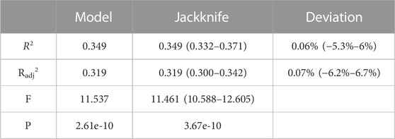
TABLE 2. Statistical parameters for the model including SST, SAM, and SAT and the test results of the jackknife method.

Figure 6 shows the simulated and observed variations and observed running mean of Weddell Sea SIC. All three prediction models generally reproduced low-frequency variability, although they were smaller extreme values of Weddell Sea SIC. The correlation coefficients between observed (seven-season running mean) Weddell Sea SIC and simulations by the models with factors in Groups 1, 2, and 3 were 0.38, 0.46, and 0.59 (0.50, 0.44, and 0.38) respectively. All the correlation coefficients passed the significant test at the 99% confidence level, suggesting that these models had generally effectively simulated the variation of Weddell Sea SIC during 1979–2012. The correlation coefficient between the observed seven-season running mean Weddell Sea SIC and the simulations with only oceanic factors (Eq. (6)) was the smallest and decreased after atmospheric factors contained in the prediction models (Eq.(7); (8). These facts implied that the simulation ability of the prediction models on the low frequency of Weddell Sea SIC decreased after consideration of the high-frequency atmospheric signals. Similarly, the simulations of Weddell Sea SIC were improved in the prediction models (Eq.(7); (8) by adding the atmospheric factors, suggesting better simulation ability on the low frequency of Weddell Sea SIC in the prediction model with only leading oceanic factors. This considered that the correlation coefficients between the simulated Weddell Sea SIC and the low-frequency (seven-season running mean) observed one decline after employing the atmospheric factors, that is, the improvements of the correlation coefficients between observed and simulated Weddell Sea SIC in Eqs.(7); (8) resulted from the better performance of these predictor models on high-frequency variability after using the atmospheric factors. Furthermore, the RMSE (MAE) of the three models were 0.75 (83.48), 0.72 (80.20), and 0.65 (71.39) (Table 3. These results imply that the declines of the errors resulted from better simulation of high-frequency variation of Weddell Sea SIC after adding the atmospheric factors, which supported the aforementioned conclusion. Compared with the curves of those observed, simulated Weddell Sea SIC was close to it during the periods 1980–1993 and 1996–2000 and showed a relatively large difference with that observed in 1987, 1993–1995, and 2002. Generally, simulated Weddell Sea SIC effectively reproduced the observed low-frequency variation. However, the simulated high-frequency variation of Weddell Sea SIC was not good for the low-frequency one during 1979–2012. Therefore, it is necessary to modify the models in order to improve the simulation results because there are system errors between the simulations and the observations.

FIGURE 6

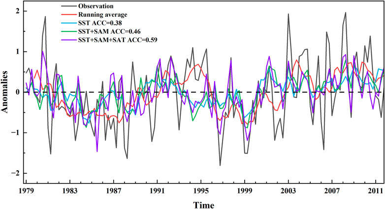
FIGURE 6. Weddell Sea SIC anomaly observation, seven-season running average of observation, and simulation by multivariate linear regression equations using three groups of predictors shown in Formulas 6, 7, and 8 in fitting period (unit: %). ACCs of those three models are indicated on the panel’s left.

TABLE 3

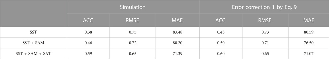
TABLE 3. Evaluations of simulated and corrected Weddell Sea SIC anomaly in the whole fitting period (1979–2012).

6 Error correction methods for the prediction models

We first analyzed the characteristics of errors in the whole fitting period. As shown in Figure 7, the errors were generally positive (negative) when the observations were positive (negative). The in-phase rate of the errors and observations was 81.6%. The errors were negative during 1981–1991 and 1996–2002 and positive during 1993–1995 and 2003–2012. The values of the errors were generally half of the observations since 2003. During the fitting period, the ratio of the errors to the observations was about 0.27, so the observed values were about 1.37 times those of simulated ones. Therefore, we developed a method to correct the high-frequency simulation, shown in Eq. (9). This error correction method enhanced the simulated Weddell Sea SIC anomaly in which the absolute values of the simulations were greater than or equal to 0.63 with 1.37 times amplification, with the others kept unchanged. We tried to set the threshold values to 0.1, 0.2, 0.3, 0.4, 0.5, 0.6, 0.7, 0.8, and 0.9 to find the changes of ACC, RMSE, and MAE. The threshold values were 0.63, corresponding to the maximal improvement of the aforementioned evaluating indicator. Therefore, we chose threshold values of 0.63 in Eq. (9).

$\begin{array}{c}{\stackrel{\sim }{SIC}}_{correction1}=\left\{\begin{array}{c}\stackrel{\sim }{SIC},\stackrel{\sim }{\left|SIC\right|}<0.63\\ 1.37\ast \stackrel{\sim }{SIC},\stackrel{\sim }{\left|SIC\right|}\ge 0.63.\end{array}\right.\end{array}(9)$

FIGURE 7

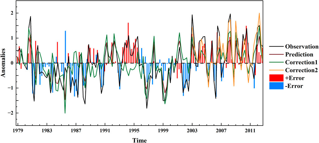
FIGURE 7. Observation, simulation by the model with Group 3 factors, and two corrections of Weddell Sea SIC anomaly in fitting period (unit: %). Correction1 represents the first error correction method shown in Eq. 9, and Correction2 represents the second method from Eq. 10. The blue and red histograms represent the positive and negative errors, respectively, between observation and simulation of SIC. The abscissa denotes the calendar year.

The simulated Weddell Sea SIC anomalies were improved after the aforementioned error correction method for 1981, 1983, 1996, 1999, 2003, 2008, and 2012, which could be found visually. The ACC, RMSE, and MAE of the three prediction models were shown in the right part of Table 3. By the correction in Eq. (9), the ACCs of these three models all increased from 0.38, 0.46, and 0.59 to 0.43, 0.50, and 0.60, respectively. The RMSEs and MAEs all decreased, except the RMSE of the prediction model under the SST, SAM, and SAT, which remained unchanged. These results suggested that this error correction method effectively improved these three prediction models. Therefore, considering only extreme values corrected by Eq. (9), the improvements of the corrected prediction models resulted from the decline errors of the extreme values.

Furthermore, considering that the observed Weddell Sea SIC anomalies were almost positive and the positive errors between the observed and simulated Weddell Sea SIC anomalies by the model with all factors were approximately half of the observations during 2003–2012, we developed the second method to correct the models in Eq. (10):

$\begin{array}{c}{\stackrel{\sim }{SIC}}_{correction2}=\left\{\begin{array}{c}\stackrel{\sim }{SIC},\stackrel{\sim }{\left|SIC\right|}<0.1\\ 1.869\ast \stackrel{\sim }{SIC},\stackrel{\sim }{\left|SIC\right|}\ge 0.1.\end{array}\right.\end{array}(10)$

The ratio of the errors to the observations was about 0.365, so the second error correction method was to enhance the simulated Weddell Sea SIC anomaly 1.869 times when the absolute values of the simulations were greater than or equal to 0.1 and to keep the others unchanged. The in-phase rate of the errors and observations was 87.5% larger than that during the whole fitting period. The ACC of the model with the factors in Group 1 increased from 0.29 to 0.31, while the other two in Groups 2 and 3 remained 0.65 and 0.64 (Table 4. The RMSEs and MAEs all decreased. These results suggested that this error correction method was also effective for improving the models. As shown in Figure 7, the second corrected Weddell Sea SIC anomalies were larger than the first and reproduced the positive observations better, such as in 2003, 2005, 2008, and 2010. In comparison, the second error correction method shown in Eq. (10) was better for enhancing the simulated extreme values during 2003–2012. The period 2003–2012 was adjacent to the predicting period. The rhythm of the errors might persist in the prediction period of 2013–2018. Therefore, this correction method was used in the next section's prediction period.

TABLE 4

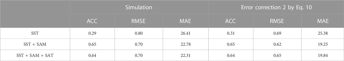
TABLE 4. Evaluations of simulated and corrected Weddell Sea SIC anomaly during 2003–2012.

7 Predictions of sudden losses of Weddell Sea SIC

The observations, predictions, and corrections for the Weddell Sea SIC anomaly in the prediction period are shown in Figure 8. The observed Weddell Sea SIC anomalies experienced a phase reversal from positive to negative over 2015–2017, which contained two sudden loss events. The first decrease of observed Weddell Sea SIC anomaly was from the peak of the austral autumn of 2015 to the average state in the austral summer of 2016, and the second decline was from the austral autumn of 2016 to the following spring. The predictions of these three models all generally reproduced the phase reversal and captured the low-frequency variability of the Weddell Sea SIC anomaly similar to the fitting period. But all the models failed to predict the time of phase reversal. The zero value of the predicted Weddell Sea SIC anomaly by the model with oceanic predictors in Group 1 lagged the observed one by two seasons and the other two by the models in Groups 2 and 3 led it by one season. The observed Weddell Sea SIC anomaly reached a peak value of 2.42% in the austral summer of 2014 and a maximum value of 2.21% in the autumn of 2015, but the amplitudes of predictions by all models were smaller and lagged the observations by one season. The observed minimum value of the Weddell Sea SIC anomaly was −2.32% in the austral spring of 2017. The predicted minimum value of the Weddell Sea SIC anomaly by the models with all factors was −1.19% synchronously and those by the other two models both were smaller and lagged the observations by one season. The models captured the extreme value in 2014, but it was smaller than the observation. The models reproduced the extreme value in 2015 and the subsequent decline and had a good performance of the recordable minimum value in 2017. The prediction ability weakened after 2018, which might be related to the length of the predictive validity. The ACCs of the three models were, respectively, 0.71, 0.68, and 0.79—shown in the left of Table 5—which all exceeded the significance test at a 99% confidence level. The RMSEs (MAEs) were, respectively, 1.05 (17.53), 1.07 (17.97), and 0.91 (15.63). Among all these models, that with all factors was the best model with oceanic factors, and SAM was worse than the one with only oceanic factors. These results indicated that Weddell Sea SAT was indispensable and could help effectively predict the sudden loss of Weddell Sea SIC during 2016–2017. As for the predicted Weddell Sea SIC anomaly by the model with all factors, the first decrease took one season from the peak value 1.03% in the austral winter of 2015, and the second decline took three seasons from the austral summer of 2016. In general, the predicted first decline of Weddell Sea SIC by the model with all factors was faster than was observed, although lagging those observed by one season. The second decline was slower and led that observed by one season. The observed and predicted Weddell Sea SIC anomaly by all models both recovered to near the average state in austral autumn of 2017.

FIGURE 8

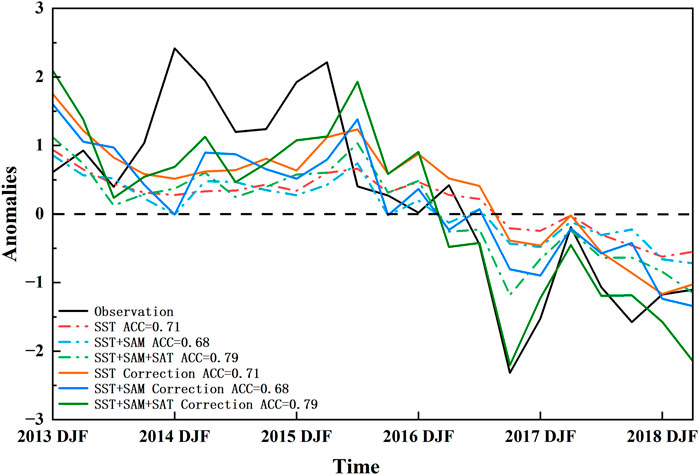
FIGURE 8. Observed, predicted, and corrected Weddell Sea SIC anomaly in prediction period (unit: %). The predicted Weddell Sea SIC anomaly refers to these predictions according to Eqs. 6–8, and the corrected ones represent the correction of Weddell Sea SIC anomaly according to Eq. 10. The colorful solid lines represent the predictions, and the dashed lines represent the corrections. The abscissa denotes the austral seasons.

TABLE 5

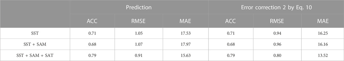
TABLE 5. Evaluations of predicted and corrected Weddell Sea SIC anomaly in the prediction period (2013–2018).

By the error correction method according to Eq. (10), the predicted Weddell Sea SIC anomalies were improved and reproduced the high-frequency variability of the observations, such as the peak values in the austral autumn of 2014 and the winter of 2015 and the minimum value in the spring of 2017. The predicted Weddell Sea SIC anomaly by the model with all factors was −2.21% in the spring of 2017 and almost perfectly predicted the variability. As shown in Table 5, the ACCs all remained unchanged and the RMSEs and the MAEs decreased after correcting. The correction models all could better predict the variability of Weddell Sea SIC. Compared with the first error correction method in Eq. (9), the second in Eq. (10) showed more effective improvement in the predicting period. Therefore, the sudden losses of Weddell Sea SIC during 2015–2017 were significantly improved by the second error correction method.

8 Possible causes of recent sudden losses of Weddell Sea SIC

A new regime shift occurred in 2013/14 (Xiao and Ren, 2023), which preceded the sudden losses of Weddell Sea SIC and might have influenced it. However, the PDO could not capture this regime shift. To better represent the signals of regime shift in the 2013/14 North Pacific SST, we employed the average of SST anomalies over the northern North Pacific (180°E−130°W, 50°–60°N), the eastern North Pacific (120°–135°W, 20°–50°N), and the northern Tropical Middle and East Pacific (110°–170°W, 10°–20°N) (according to Figure 1 of their study) to represent the PDO index in Figure 9. We also used the averaged SST anomalies to represent the PDO index in the prediction and correction models. The coefficient, ACC, RMSE, and MAE of the prediction models were very similar (not shown). Therefore, it was reasonable that the averaged SST anomalies in the North Pacific were used to indicate the PDO index in this section.

FIGURE 9

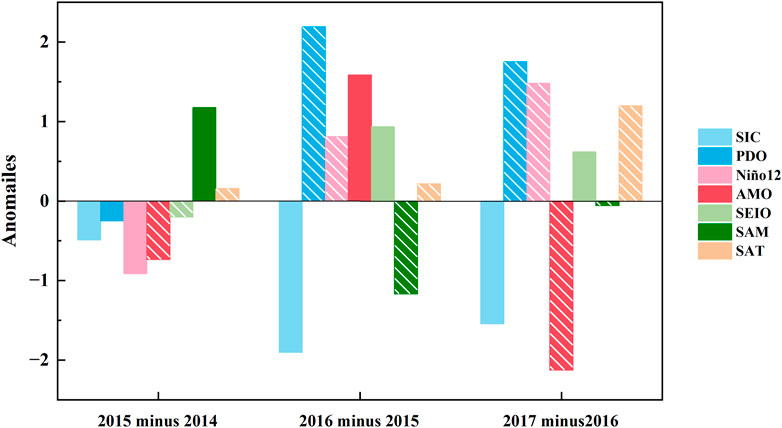
FIGURE 9. Changes of Weddell Sea SIC in austral summer and the predictors at corresponding lead time of 2015–2017 compared with their values over the previous year. For example, the symbol “2015 minus 2014” of SIC indicates the difference of Weddell Sea SIC between 2015 and 2014. The symbol “2015 minus 2014” of AMO indicates the difference of the AMO index at the season leading 11 seasons of 2015 summer and that of 2014. White diagonal markers indicate positive contributions.

Figure 9 shows the difference in the Weddell Sea SIC anomaly in the austral summer between the neighboring years and the potential factors at individual leading times before it. The difference in the SIC anomaly between 2015 and 2014 showed a negative anomaly of 0.5%. The PDO, AMO, Niño12, and SEIO SST anomalies also reduced, while the SAM and Weddell Sea SAT anomalies increased. Considering the positive and negative relationships between them and Weddell Sea SIC, this suggested that the AMO, SEIO SST, and SAT made positive contributions to the decrease of the Weddell Sea SIC anomaly. Regarding the difference between 2016 and 2015, the Weddell Sea SIC anomaly sharply reduced by up to 1.9, and the PDO, AMO, Niño12, and SEIO SSTs and Weddell Sea SAT anomalies increased while the SAM anomaly decreased. These facts implied that the positive contributions of declining Weddell Sea SIC in 2016 were from the PDO, Niño12 SST, SAM, and SAT and that the negative contributions were from the other factors. The PDO anomaly had the largest positive change. In terms of the difference between 2017 and 2016, the Weddell Sea SIC anomaly decreased by 1.5%. The AMO, PDO, Niño12 SST, SAM, and Weddell Sea SAT showed positive contributions from decreased Weddell Sea SIC in 2017. However, the SEIO SST provided a negative contribution. According to the aforementioned findings, the main factors influencing the sudden losses of Weddell Sea SIC in 2016 (2017) were the PDO, Niño12 SST, SAM, and SAT (AMO, PDO, Niño12 SST, SAM, SAT). The SAT was the consistently positive contributor during 2015–2017. The PDO, Niño12 SST, SAM, and SAT were the common factors which positively contributed to the two sudden losses of Weddell Sea SIC in 2016 and 2017. The AMO contributed negatively to the sudden loss of Weddell Sea SIC in 2016 but made a stronger positive contribution in 2017.

9 Conclusion and discussion

This study focused on recent sudden declines of SIC in the Weddell Sea. We noted that sea-ice in the Antarctic has reduced in recent years and that the Weddell Sea was the primary area of this. The Weddell Sea SIC anomaly was in a long-term increasing trend, but after reaching peak in 2014, it was on a record-breaking downward trend, falling from 2.21% to −2.32%. The Weddell Sea SIC anomaly was positive until 2014 and then almost entirely negative in 2017.

We explored the potential contributions of the leading atmospheric and oceanic factors to these losses in Weddell Sea sea-ice. Six potential influencing factors were identified by calculating the leading–lagged correlation coefficients. The AMO led Weddell Sea SIC by eleven seasons, the PDO by ten, the Niño12 and SEIO SSTs by five, the SAM by three seasons, and the SAT over the Weddell Sea most significantly correlated with the SIC simultaneously.

These six factors were divided into three groups to establish the multiple linear regression models during the fitting period 1979–2012. The groups of potential predictors aimed to explore the effects of the leading oceanic factors (including the PDO, AMO, SEIO, and Niño12 SSTs), the combination of the aforementioned leading oceanic and an atmospheric factor (SAM), and a leading oceanic factor, SAM, and simultaneous Weddell Sea SAT. These three groups of potential factors were employed to establish each prediction model for 1979–2012, which exceeded the 99.9% confidence level of F- and jackknife tests. All these three prediction models effectively reproduced the low-frequency variation of the Weddell Sea SIC anomaly. We developed two error correction methods to improve the simulated extreme values of Weddell Sea SIC. The ACC, RMSE, and MAE were obviously improved after correcting. The second error correction method had better performance in improving the models' accuracy.

We examined the predicted Weddell Sea SIC anomaly during the prediction period 2013–2018. The three models captured the phase reversal and low-frequency variability of Weddell Sea SIC anomalies. The models all predicted the sudden losses of sea-ice in the Weddell Sea, and the model with all factors had the best performance. The predicted Weddell Sea SIC anomalies were improved through the second error correction method, with the ACCs remaining unchanged and the RMSEs and the MAEs decreasing.

The models captured the variability of Weddell Sea SIC anomalies, especially after correction, and the six factors we selected had an important influence on the losses of Weddell Sea SIC. The AMO, SEIO SST, and SAT made positive contributions to the decline of the Weddell Sea SIC anomaly during 2014–2015. In 2015–2016, the positive contributions were from the PDO, Niño12 SST, SAM, and SAT. In 2016–2017, all the factors except the SEIO SST had a jointly positive influence on the decline of Weddell Sea SIC. The Weddell Sea SAT was the most primary factor and positive contributor.

The Weddell Sea SIC anomaly increased in the early 1990s and reached the maximum value of 1.07% in the austral winter of 1995. It then experienced a rapid and sharp decline, approaching the climatic average of −0.03% in the austral summer of 1996 and a low value of −1.81% in the austral spring of 1996. When Weddell Sea SIC decreased dramatically, the PDO and SAT increased, the Niño12 SST was almost unchanged, and the AMO, SEIO SST, and SAM decreased. Considering the positive and negative relationships between them and Weddell Sea SIC, it suggested that all factors except Nino12 SST made positive contributions to the decrease of Weddell Sea SIC.

The two error correction methods used in this study statistically enhanced the high values of predictions in the prediction period based on the characteristics of errors in the fitting period. There are many other effective post-processing methods to revise the results produced by the prediction models, such as machine learning. Using other efficient post-processing methods may result in higher accuracy.

Sudden recent decreases of sea-ice in the Weddell Sea and even the entire Antarctic occurred after a hiatus in global warming. It is not yet known whether there is a clear connection between the two events or only a coincidence. The link between the changes in sea-ice and in the global climate system still needs to be explored.

Moreover, although these factors can predict the losses of Weddell Sea SIC to some extent, we still do not understand that how they affect sea-ice, at which time scale, whether they are influenced directly or indirectly by other factors, or how long the effects would last. More discussion and analysis is needed regarding the interactions between sea-ice and predictors. In addition to the six predictors selected in this study, there may be further related factors in the internal climate system and external factors that play an important role in Antarctic sea-ice decrease. These considerations merit further and deeper research.

Data availability statement

The original contributions presented in the study are included in the article/Supplementary Material; further inquiries can be directed to the corresponding author.

Author contributions

H-JZ performed the statistical analysis and wrote the first draft of the manuscript. DX contributed to conception and design of the study and wrote sections of the manuscript. All authors gave the advices and approved the submitted version.

Funding

This work was jointly supported by the Strategic Priority Research Program of the Chinese Academy of Sciences (XDA20100300) and the Second Tibetan Plateau Scientific Expedition and Research (STEP) program (2019QZKK0105), a National Science Foundation of China grant (42175053), and the Natural Science Foundation of Shanghai (21ZR1457600).

Conflict of interest

The authors declare that the research was conducted in the absence of any commercial or financial relationships that could be construed as a potential conflict of interest.

Publisher’s note

All claims expressed in this article are solely those of the authors and do not necessarily represent those of their affiliated organizations, or those of the publisher, the editors, and the reviewers. Any product that may be evaluated in this article, or claim that may be made by its manufacturer, is not guaranteed or endorsed by the publisher.

References

Bintanja, R., van Oldenborgh, G. J., Drijfhout, S. S., Wouters, B., and Katsman, C. A. (2013). Important role for ocean warming and increased ice-shelf melt in Antarctic sea-ice expansion. Nat. Geosci. 6 (5), 376–379. doi:10.1038/ngeo1767

CrossRef Full Text | Google Scholar

Chen, D., and Yuan, X. (2004). A Markov model for seasonal forecast of antarctic Sea Ice. J. Clim. 172 (16), 3156–3168. doi:10.1175/1520-0442(2004)017<3156:ammfsf>2.0.co;2

CrossRef Full Text | Google Scholar

Comiso, J. C., Gersten, R. A., Stock, L. V., Turner, J., Perez, G. J., and Cho, K. (2017). Positive trend in the antarctic Sea Ice cover and associated changes in surface temperature. J. Clim. 30 (6), 2251–2267. doi:10.1175/jcli-d-16-0408.1

PubMed Abstract | CrossRef Full Text | Google Scholar

Cruz-García, R., Guemas, V., Chevallier, M., and Massonnet, F. (2019). An assessment of regional sea-ice predictability in the Arctic ocean. Clim. Dyn. 53 (1-2), 427–440. doi:10.1007/s00382-018-4592-6

CrossRef Full Text | Google Scholar

Dou, J., and Zhang, R. (2022). Weakened relationship between ENSO and Antarctic sea-ice in recent decades. Clim. Dyn. doi:10.1007/s00382-022-06364-4

CrossRef Full Text | Google Scholar

Eayrs, C., Li, X., Raphael, M. N., and Holland, D. M. (2021). Rapid decline in Antarctic sea-ice in recent years hints at future change. Nat. Geosci. 14 (7), 460–464. doi:10.1038/s41561-021-00768-3

CrossRef Full Text | Google Scholar

Efron, B. (1979). Bootstrap methods: Another look at the Jackknife. Ann. Statistics 7 (1), 1–26. doi:10.1214/aos/1176344552

CrossRef Full Text | Google Scholar

Enfield, D. B., Mestas-Nunez, A. M., and Trimble, P. J. (2001). The Atlantic Multidecadal Oscillation and its relation to rainfall and river flows in the continental U.S. Geophys. Res. Lett. 28, 2077–2080. doi:10.1029/2000gl012745

CrossRef Full Text | Google Scholar

Guemas, V., Blanchard-Wrigglesworth, E., Chevallier, M., Day, J. J., Déqué, M., Doblas-Reyes, F. J., et al. (2016). A review on Arctic sea-ice predictability and prediction on seasonal to decadal time-scales. Q. J. R. Meteorological Soc. 142 (695), 546–561. doi:10.1002/qj.2401

CrossRef Full Text | Google Scholar

Haumann, F. A., Gruber, N., Munnich, M., Frenger, I., and Kern, S. (2016). Sea-ice transport driving Southern Ocean salinity and its recent trends. Nature 537 (7618), 89–92. doi:10.1038/nature19101

PubMed Abstract | CrossRef Full Text | Google Scholar

Hersbach, H., Bell, B., Berrisford, P., Hirahara, S., Horányi, A., Muñoz-Sabater, J., et al. (2020). The ERA5 global reanalysis. Q. J. R. Meteorological Soc. 146, 1999–2049. doi:10.1002/qj.3803

CrossRef Full Text | Google Scholar

Holland, M. M., Blanchard-Wrigglesworth, E., Kay, J., and Vavrus, S. (2013). Initial-value predictability of antarctic sea-ice in the community climate system model 3. Geophys. Res. Lett. 40 (10), 2121–2124. doi:10.1002/grl.50410

CrossRef Full Text | Google Scholar

Hosking, J. S., Marshall, G. J., Phillips, T., Bracegirdle, T. J., and Turner, J. (2013). An initial assessment of antarctic Sea Ice extent in the CMIP5 models. J. Clim. 26 (5), 1473–1484. doi:10.1175/jcli-d-12-00068.1

CrossRef Full Text | Google Scholar

Huang, J. (2004). Meteorological statistics method. Version 3. Beijing: China Meteorological Press.

Google Scholar

Jenouvrier, S., Che-Castaldo, J., Wolf, S., Holland, M., Labrousse, S., LaRue, M., et al. (2021). The call of the emperor penguin: Legal responses to species threatened by climate change. Glob. Chang. Biol. 27 (20), 5008–5029. doi:10.1111/gcb.15806

PubMed Abstract | CrossRef Full Text | Google Scholar

Jones, D. A., and Simmonds, I. (1993). A climatology of Southern Hemisphere extratropical cyclones. Clim. Dyn. 9 (3), 131–145. doi:10.1007/bf00209750

CrossRef Full Text | Google Scholar

Kidston, J., Scaife, A. A., Hardiman, S. C., Mitchell, D. M., Butchart, N., Baldwin, M. P., et al. (2015). Stratospheric influence on tropospheric jet streams, storm tracks and surface weather. Nat. Geosci. 8 (6), 433–440. doi:10.1038/ngeo2424

CrossRef Full Text | Google Scholar

Kim, Y. J., Kim, H. C., Han, D., Lee, S., and Im, J. (2020). Prediction of monthly Arctic sea-ice concentrations using satellite and reanalysis data based on convolutional neural networks. Cryosphere 14 (3), 1083–1104. doi:10.5194/tc-14-1083-2020

CrossRef Full Text | Google Scholar

King, J. (2014). Climate science: A resolution of the antarctic paradox. Nature 505 (7484), 491–492. doi:10.1038/505491a

PubMed Abstract | CrossRef Full Text | Google Scholar

King, J., and Turner, J. (1997). Antarctic meteorology and climatology (cambridge atmospheric and space science series). Cambridge: Cambridge University Press.

Google Scholar

Kitade, Y., Shimada, K., Tamura, T., Williams, G. D., Aoki, S., Fukamachi, Y., et al. (2014). Antarctic bottom water production from the vincennes bay polynya, East Antarctica. Geophys. Res. Lett. 41 (10), 3528–3534. doi:10.1002/2014gl059971

CrossRef Full Text | Google Scholar

Kusahara, K., Reid, P., Williams, G. D., Massom, R., and Hasumi, H. (2018). An ocean-sea-ice model study of the unprecedented Antarctic sea-ice minimum in 2016. Environ. Res. Lett. 13 (8), 084020. doi:10.1088/1748-9326/aad624

CrossRef Full Text | Google Scholar

Kwok, R., and Comiso, J. C. (2002). Southern Ocean climate and Sea Ice anomalies associated with the southern oscillation. J. Clim. 152 (5), 487–501. doi:10.1175/1520-0442(2002)015<0487:socasi>2.0.co;2

CrossRef Full Text | Google Scholar

Lecomte, O., Goosse, H., Fichefet, T., de Lavergne, C., Barthelemy, A., and Zunz, V. (2017). Vertical ocean heat redistribution sustaining sea-ice concentration trends in the Ross Sea. Nat. Commun. 8 (1), 258. doi:10.1038/s41467-017-00347-4

PubMed Abstract | CrossRef Full Text | Google Scholar

Li, S., Han, Z., Liu, N., Zhang, C., and Cai, H. (2021). A review of the researches on the record low Antarctic sea-ice in 2016 and its formation mechanisms. Haiyang Xuebao 43 (7), 1–10. doi:10.12284/hyxb2021119

CrossRef Full Text | Google Scholar

Li, X., Holland, D. M., Gerber, E. P., and Yoo, C. (2014). Impacts of the North and tropical Atlantic Ocean on the antarctic Peninsula and sea-ice. Nature 505 (7484), 538–542. doi:10.1038/nature12945

PubMed Abstract | CrossRef Full Text | Google Scholar

Liu, G., Song, W., and Zhu, Y. (2013). A statistical prediction method for an East Asian winter monsoon index reflecting winter temperature changes over the Chinese mainland. Acta Meteorol. Sin. 71 (2), 275–285. doi:10.11676/qxxb2013.025

CrossRef Full Text | Google Scholar

Liu, J., Yuan, X., Rind, D., and Martinson, D. G. (2002). Mechanism study of the ENSO and southern high latitude climate teleconnections. Geophys. Res. Lett. 29 (14), 24–42424. doi:10.1029/2002gl015143

CrossRef Full Text | Google Scholar

Liu, Q., Zhang, R., Wang, Y., Yan, H., and Hong, M. (2021a). Daily prediction of the arctic Sea Ice concentration using reanalysis data based on a convolutional LSTM network. J. Mar. Sci. Eng. 9 (3), 330. doi:10.3390/jmse9030330

CrossRef Full Text | Google Scholar

Liu, Y., Bogaardt, L., Attema, J., and Hazeleger, W. (2021b). Extended range arctic Sea Ice forecast with convolutional long-short term memory networks. Mon. Weather Rev. 149 (6), 1673–1693. doi:10.1175/mwr-d-20-0113.1

CrossRef Full Text | Google Scholar

Mantua, N. J., Hare, S. R., Zhang, Y., Wallace, J. M., and Francis, R. C. (1997). A pacific interdecadal climate oscillation with impacts on salmon production. Bull. Am. Meteorological Soc. 78 (6), 1069–1079. doi:10.1175/1520-0477(1997)078<1069:Apicow>2.0.Co;2

CrossRef Full Text | Google Scholar

Mayewski, P. A., Meredith, M. P., Summerhayes, C. P., Turner, J., Worby, A., Barrett, P. J., et al. (2009). State of the antarctic and southern ocean climate system. Rev. Geophys. 47 (1). doi:10.1029/2007rg000231

CrossRef Full Text | Google Scholar

Meehl, G. A., Arblaster, J. M., Bitz, C. M., Chung, C. T. Y., and Teng, H. (2016). Antarctic sea-ice expansion between 2000 and 2014 driven by tropical Pacific decadal climate variability. Nat. Geosci. 9 (8), 590–595. doi:10.1038/ngeo2751

CrossRef Full Text | Google Scholar

Meehl, G. A., Arblaster, J. M., Chung, C. T. Y., Holland, M. M., DuVivier, A., Thompson, L., et al. (2019). Sustained ocean changes contributed to sudden Antarctic sea-ice retreat in late 2016. Nat. Commun. 10 (1), 14. doi:10.1038/s41467-018-07865-9

PubMed Abstract | CrossRef Full Text | Google Scholar

Meier, W. N., Fetterer, F., Savoie, M., Mallory, S., Duerr, R., and Stroeve, J. (2017). NOAA/NSIDC climate data record of passive Microwave Sea Ice concentration. Version 3. doi:10.7265/N59P2ZTG

CrossRef Full Text | Google Scholar

Meyer, B., Freier, U., Grimm, V., Groeneveld, J., Hunt, B. P. V., Kerwath, S., et al. (2017). The winter pack-ice zone provides a sheltered but food-poor habitat for larval Antarctic krill. Nat. Ecol. Evol. 1 (12), 1853–1861. doi:10.1038/s41559-017-0368-3

PubMed Abstract | CrossRef Full Text | Google Scholar

Mo, K. C., and Paegle, J. N. (2001). The Pacific-South American modes and their downstream effects. Int. J. Climatol. 21 (10), 1211–1229. doi:10.1002/joc.685

CrossRef Full Text | Google Scholar

Mohammadi-Aragh, M., Goessling, H. F., Losch, M., Hutter, N., and Jung, T. (2018). Predictability of Arctic sea-ice on weather time scales. Sci. Rep. 8 (1), 6514. doi:10.1038/s41598-018-24660-0

PubMed Abstract | CrossRef Full Text | Google Scholar

Morice, C. P., Kennedy, J. J., Rayner, N. A., Winn, J. P., Hogan, E., Killick, R. E., et al. (2021). An updated assessment of near-surface temperature change from 1850: The HadCRUT5 data set. J. Geophys. Res. Atmos. 126 (3). doi:10.1029/2019jd032361

CrossRef Full Text | Google Scholar

Nan, S., and Li, J. (2003). The relationship between the summer precipitation in the Yangtze River valley and the boreal spring Southern Hemisphere annular mode. Geophys. Res. Lett. 30 (24). doi:10.1029/2003gl018381

CrossRef Full Text | Google Scholar

Ohshima, K. I., Fukamachi, Y., Williams, G. D., Nihashi, S., Roquet, F., Kitade, Y., et al. (2013). Antarctic Bottom Water production by intense sea-ice formation in the Cape Darnley polynya. Nat. Geosci. 6 (3), 235–240. doi:10.1038/ngeo1738

CrossRef Full Text | Google Scholar

Parkinson, C. L. (2019). A 40-y record reveals gradual Antarctic sea-ice increases followed by decreases at rates far exceeding the rates seen in the Arctic. Proc. Natl. Acad. Sci. U. S. A. 116 (29), 14414–14423. doi:10.1073/pnas.1906556116

PubMed Abstract | CrossRef Full Text | Google Scholar

Parkinson, C. L., and DiGirolamo, N. E. (2016). New visualizations highlight new information on the contrasting Arctic and Antarctic sea-ice trends since the late 1970s. Remote Sens. Environ. 183, 198–204. doi:10.1016/j.rse.2016.05.020

CrossRef Full Text | Google Scholar

Peng, G., Meier, W. N., Scott, D. J., and Savoie, M. H. (2013). A long-term and reproducible passive microwave sea-ice concentration data record for climate studies and monitoring. Earth Syst. Sci. Data 5 (2), 311–318. doi:10.5194/essd-5-311-2013

CrossRef Full Text | Google Scholar

Polvani, L. M., and Smith, K. L. (2013). Can natural variability explain observed antarctic sea-ice trends? New modeling evidence from CMIP5. Geophys. Res. Lett. 40 (12), 3195–3199. doi:10.1002/grl.50578

CrossRef Full Text | Google Scholar

Purich, A., and England, M. H. (2019). Tropical teleconnections to antarctic Sea Ice during austral spring 2016 in coupled pacemaker experiments. Geophys. Res. Lett. 46 (12), 6848–6858. doi:10.1029/2019gl082671

CrossRef Full Text | Google Scholar

Pyper, B. J., and Peterman, R. M. (1998). Comparison of methods to account for autocorrelation in correlation analyses of fish data. J. Fish. Aquatic Sci. 55, 2127–2140. doi:10.1139/f98-104

CrossRef Full Text | Google Scholar

Rayner, N. A. (2003). Global analyses of sea surface temperature, sea-ice, and night marine air temperature since the late nineteenth century. J. Geophys. Res. 108 (14), 4407. doi:10.1029/2002jd002670

CrossRef Full Text | Google Scholar

Saji, N. H., Goswami, B. N., Vinayachandran, P. N., and Yamagata, T. (1999). A dipole mode in the tropical Indian Ocean. Nature 401, 360–363. doi:10.1038/43854

PubMed Abstract | CrossRef Full Text | Google Scholar

Schlosser, E., Haumann, F. A., and Raphael, M. N. (2018). Atmospheric influences on the anomalous 2016 Antarctic sea-ice decay. Cryosphere 12 (3), 1103–1119. doi:10.5194/tc-12-1103-2018

CrossRef Full Text | Google Scholar

Seo, K. H., and Son, S. W. (2012). The global atmospheric circulation response to tropical diabatic heating associated with the madden–julian oscillation during northern winter. J. Atmos. Sci. 69 (1), 79–96. doi:10.1175/2011jas3686.1

CrossRef Full Text | Google Scholar

Serreze, M. C., and Stroeve, J. (2015). Arctic sea-ice trends, variability and implications for seasonal ice forecasting. Philos. Trans. A Math. Phys. Eng. Sci. 373, 20140159. doi:10.1098/rsta.2014.0159

PubMed Abstract | CrossRef Full Text | Google Scholar

Shu, Q., Wang, Q., Song, Z., Qiao, F., Zhao, J., Chu, M., et al. (2020). Assessment of Sea Ice extent in CMIP6 with comparison to observations and CMIP5. Geophys. Res. Lett. 47 (9). doi:10.1029/2020gl087965

CrossRef Full Text | Google Scholar

Stuecker, M. F., Bitz, C. M., and Armour, K. C. (2017). Conditions leading to the unprecedented low Antarctic sea-ice extent during the 2016 austral spring season. Geophys. Res. Lett. 44 (17), 9008–9019. doi:10.1002/2017gl074691

CrossRef Full Text | Google Scholar

Stuecker, M. F., Jin, F., Timmermann, A., and McGregor, S. (2015). Combination mode dynamics of the anomalous northwest Pacific anticyclone. J. Clim. 28 (3), 1093–1111. doi:10.1175/jcli-d-14-00225.1

CrossRef Full Text | Google Scholar

Swart, S., Campbell, E. C., Heuze, C. H., Johnson, K., Lieser, J. L., Massom, R., et al. (2018). Return of the maud rise polynya: Climate litmus or sea-ice anomaly? Bull. Am. Meteorological Soc. 99 (8), 188–S310. doi:10.1175/2018BAMSStateoftheClimate.1

CrossRef Full Text | Google Scholar

Turner, J., and Comiso, J. (2017). Solve Antarctica's sea-ice puzzle. Nature 547 (7663), 275–277. doi:10.1038/547275a

PubMed Abstract | CrossRef Full Text | Google Scholar

Turner, J., Guarino, M. V., Arnatt, J., Jena, B., Marshall, G. J., Phillips, T., et al. (2020). Recent decrease of summer Sea Ice in the Weddell Sea, Antarctica. Geophys. Res. Lett. 47 (11). doi:10.1029/2020gl087127

CrossRef Full Text | Google Scholar

Turner, J., Hosking, J. S., Bracegirdle, T. J., Marshall, G. J., and Phillips, T. (2015). Recent changes in antarctic Sea Ice. Philos. Trans. A Math. Phys. Eng. Sci. 373, 20140163. doi:10.1098/rsta.2014.0163

PubMed Abstract | CrossRef Full Text | Google Scholar

Turner, J., Phillips, T., Marshall, G. J., Hosking, J. S., Pope, J. O., Bracegirdle, T. J., et al. (2017). Unprecedented springtime retreat of Antarctic sea-ice in 2016. Geophys. Res. Lett. 44 (13), 6868–6875. doi:10.1002/2017gl073656

CrossRef Full Text | Google Scholar

Wang, G., Hendon, H. H., Arblaster, J. M., Lim, E. P., Abhik, S., and van Rensch, P. (2019). Compounding tropical and stratospheric forcing of the record low Antarctic sea-ice in 2016. Nat. Commun. 10 (1), 13. doi:10.1038/s41467-018-07689-7

PubMed Abstract | CrossRef Full Text | Google Scholar

Wang, L., Yuan, X., and Li, C. (2018). Subseasonal forecast of Arctic sea-ice concentration via statistical approaches. Clim. Dyn. 52 (7-8), 4953–4971. doi:10.1007/s00382-018-4426-6

CrossRef Full Text | Google Scholar

Xiao, D., Li, Y., Fan, S., Zhang, R., Sun, J., and Wang, Y. (2014). Plausible influence of Atlantic Ocean SST anomalies on winter haze in China. Theor. Appl. Climatol. 122 (1-2), 249–257. doi:10.1007/s00704-014-1297-6

CrossRef Full Text | Google Scholar

Xiao, D., and Ren, H. (2023). A regime shift in North Pacific annual mean sea surface temperature in 2013/14. Front. Earth Sci. 10, 987349. doi:10.3389/feart.2022.987349

CrossRef Full Text | Google Scholar

Xiao, D., Zhao, P., and Ren, H. (2021). Climatic factors contributing to interannual and interdecadal variations in the meridional displacement of the East Asian jet stream in boreal winter. Atmos. Res. 264, 105864. doi:10.1016/j.atmosres.2021.105864

CrossRef Full Text | Google Scholar

Yuan, X., Chen, D., Li, C., Wang, L., and Wang, W. (2016). Arctic Sea ice seasonal prediction by a linear Markov model. J. Clim. 29 (22), 8151–8173. doi:10.1175/jcli-d-15-0858.1

CrossRef Full Text | Google Scholar