Numerical study of extreme waves driven by synthetic tropical cyclones in the northwest Pacific Ocean

Extreme waves induced by extreme tropical cyclones (TCs) with a very strong intensity threaten marine production and transportation. In this paper, six tropical cyclones with a typical track and extremely strong intensity were synthesized to study the extreme waves. The data on TC tracks were extracted from the China Meteorological Administration. The historic TCs from 1949 to 2018 were classified into six groups according to their tracks, and a representative track was synthesized for each group of TCs. We applied an extremely strong intensity to the tracks for studying the extreme wave field. The synthesized track of typical track cyclones (TTCs) was based on the maximum probability of the translation distance and direction of the TC center according to historical data. The central pressure (P_c) was used to represent the TC intensity and was studied at the recurrence periods of 100, 1,000, and 10,000 years. The synthetic TC with a representative track and extremely strong intensity was called a typical tropical cyclone (TTC). The extreme wave fields driven by TTCs were simulated by Simulating Waves Nearshore (SWAN). The wind field driving the waves was calculated using the Holland parametric wind model and was well-verified with observations. This paper calculated the extreme H_s and T_p values of the return periods of 100, 1,000, and 10,000 years for six types of TTCs. It was found that the extreme H_s values were very different for each TTC. The highest H_s could reach 31.3 m in the recurrence period of 10,000 years. Followed by TTC-I with 18 m, TTC-VI was the weakest with less than 10 m. The TC track position frequency and its spatial variation of extreme intensity were discussed. The synthetic tracks were representative, and the intensity could be influenced by spatial variation. In the end, four historical typhoons with great intensity, wide impact, and serious disaster-causing effects were selected to compare with TTC. This paper can provide guidance for maritime planners.

1 Introduction

Extreme TCs along with strong winds, huge waves, storm surges, and heavy rainfall are the primary causes of most marine disasters that lead to huge economic losses and casualties each year (Wu et al., 2014; Wu G. et al., 2018; Yan et al., 2020; Shi et al., 2021). A few super TCs that were never reported before have occurred in both the Pacific Ocean and the Atlantic Ocean in recent years (Tajima et al., 2014; Berg 2016; Cox et al., 2019). Moreover, the intensity of TCs in the future will probably increase as a result of climate change (Yasuda et al., 2014; Mori and Takemi, 2016). Tropical cyclones (TCs) in the northwest Pacific Ocean frequently affect China, Japan, and Southeast Asian countries (Yang et al., 2019). The wave fields formed by TCs are operational for predicting potentially hazardous conditions for ship navigation and coastal areas and for countries in the path of severe tropical cyclones, where marine structures and ships are under serious threat from giant waves. The impact of extreme typhoons on damage levels makes extreme typhoons a critical factor in marine structure design projects.

Numerical models, including SWAN (Simulating WAves Nearshore), WAM (wind wave model), WW3 (WaveWatch-III), and UMWM (University of Miami Wave Model), have been developed for simulating the wave field in the past decades. All these models are third-generation wave models that are based on the balance equation of dynamic spectral density, considering the non-linear physical process. It is known that the model configuration is critical for accurate simulation on account of parameter sensitivity (Xu et al., 2017; Wu Z. Y et al., 2018). Therefore, the SWAN model, which calculates the sensitive parameters of the drag coefficient, depth-induced wave breaking, and wind field very well in a simulation, is better than the other models in the near-shore wave simulations (Fan et al., 2009; Umesh and Swain, 2018; Wu Z. Y et al., 2018; Qiao et al., 2019; Umesh and Behera, 2020; Xu et al., 2020). Apart from the unstructured grid option which can be used to simulate the large domain embedding high coastal resolution in a high efficiency without nesting (Zijlema, 2010), the coupled model in SWAN considering the interaction between different dynamic factors enables the more accurate simulation (Fan et al., 2012; Hong et al., 2018; Prakash and Pant, 2020). Moreover, the blended wind field of the reanalyzed wind field and parametric wind field in SWAN improved the simulation results significantly (Shao et al., 2018; Hsiao et al., 2020).

Although the numerical simulation of the wave field under a certain TC has been studied by many researchers, including Tolman et al. (2005), Wang (2005), and Lalbeharry et al. (2009), neither the effects of a given TC on a given area nor the intensity quadrature is distinguished. The purpose of this paper is to quantify the intensity of TCs by simulating waves under extreme TCs along typical paths in the Northwest Pacific. The tracks of TCs in the Northwest Pacific were divided into six typical types according to their passing areas and shapes. The typical tracks that are most likely to happen in each type were synthesized. The wave field under synthetic TCs was simulated by SWAN.

2 Data

The datasets used in this study are from the China Meteorological Administration Shanghai Typhoon Institute (CMA-STI). This dataset records the TCs that occurred in the Northwest Pacific. The recorded data in every 6 h contain time, intensity category, central pressure (P_c), and the maximum wind speed of TC when the intensity was no less than the tropical depression (Ying et al., 2014). To study the extreme TCs, data from 1949 to 2018, during which the strongest intensity of TCs reached a tropical storm, were selected as samples. Consequently, the total number was 1908.

Knowing that the characteristics and influencing regions vary with TCs’ track, the northwest Pacific Ocean was divided into four subareas. As shown in Figure 1, Rumpf et al. (2007) divided the TCs, which occurred in the Northwest Pacific into six groups according to the subareas of formation, passing-by, and dissipation. The southeast, southwest, northwest, and northeast subareas were individually named No.1–No.4. The TC group classification parameters are listed in Table 1. Groups I and IV did not have TC landfall. Group V had few TCs that influenced Asia. Therefore, groups II, III, and VI affected Asian countries severely with a large frequency. The TCs in each of the three groups were further divided into landfalling China and non-landfalling China types. Thus, six kinds of typical TCs, sTTC-I–TTC-VI in Section 3.1, were identified, as shown in Figure 2. TCs of Type-I formed in the open sea at low latitudes and moved northwest to the South China Sea or south to the East China Sea, influencing the southern provinces of China, such as Guangdong, Guangxi, Hainan, Fujian, and Taiwan. In contrast, TCs of Type-II did not land in China, but it still had a serious impact in the South China Sea and Southeast Asia. TCs of Type-III and Type-IV tended to recurve between 20 °N and 30 °N. The number and the characteristic of recurving of the latter type were individually much larger and more apparently. These two types of TCs had significant impacts on the east of China and Japan, whilst TCs of Type-V and Type-VI influenced South China and Southeast Asia with a shorter duration and weaker intensity.

FIGURE 1

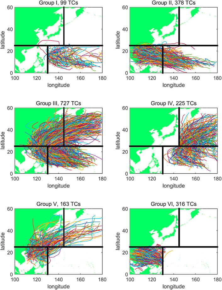
FIGURE 1. Six groups of TCs divided by Rumpf et al. (2007) in the Northwest Pacific.

TABLE 1

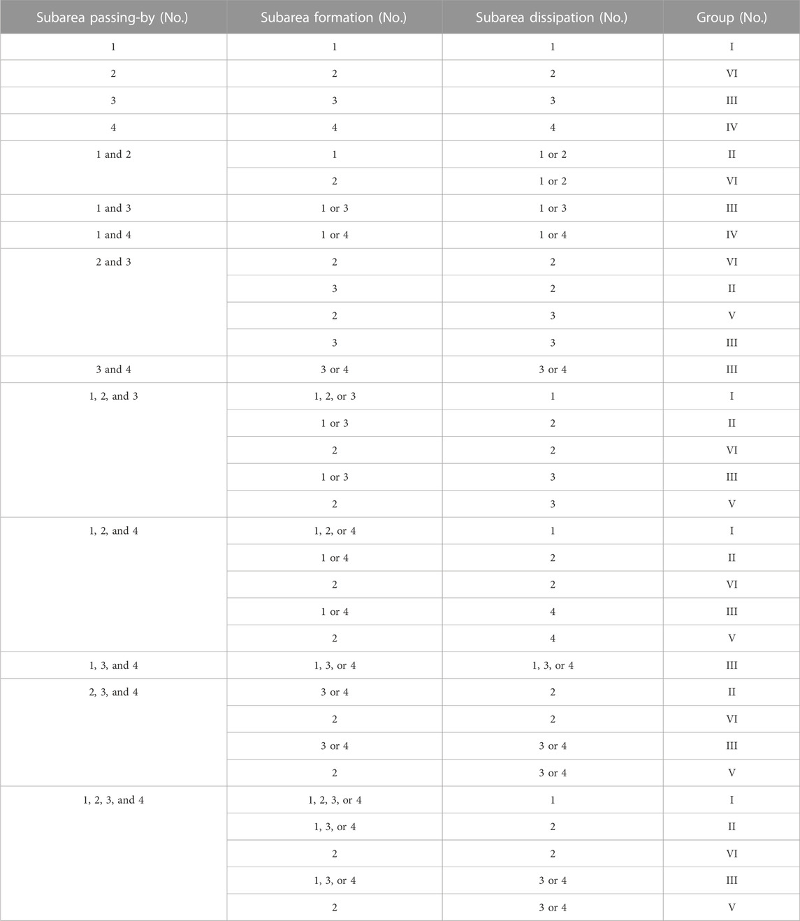
TABLE 1. Rules of TC classification.

FIGURE 2

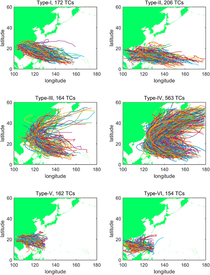
FIGURE 2. Six kinds of typical TC tracks (Type-I is the landfalling China TCs of Group II, Type-II is the no-landfalling China TCs of Group II, Type-III is the landfalling China TCs of Group III, Type-IV is the non-landfalling China TC of Group III, Type-V is the landfalling China TCs of Group VI, and Type-VI is the non-landfalling China TCs of Group VI).

3 Models

3.1 Typical extreme TC synthetic model

Since the occurrence of super TCs (with a recurrence period of more than 1,000 years) is rare and random, the synthesis of each type of super TCs was performed according to statistical methods. In the synthetic TC, its track was described as a polyline with the positions of the TC center as the vertex, as shown in Figure 3. The position of the TC center was recorded every 6 h. Knowing that the moving characteristics of TC were determined by the translation distance (TD_6h) and direction (θ) between two adjacent points, the track could be synthesized once TD_6h and θ were obtained in all steps. Typicality was considered as the maximum probability of each type of TC moving TD_6h and θ. Therefore, the occurrence frequency in spatial distribution was calculated by a non-parametric method according to the historic TCs. This is because the non-parametric method does not have a fixed form of probability density function, and it is more suitable than the parametric method for irregular sample distributions. Integrating the probability density function gets the cumulative probability F, and T = 1/(1–F) is the recurrence period.

FIGURE 3

FIGURE 3. Schematic diagram of the synthetic TC track.

The point with the maximum historic forming frequency was chosen as the start point of a typical TC for each type. Next, both TD_6h and θ in each step were fitted for each step using a non-parametric method with a Gaussian kernel function. The samples were collected from the historical data with a grid box of 2° × 2°, centered on the simulated track point, as shown in Figure 3. TD_6h and θ, owing to the maximum probabilities, were calculated. By repeating the aforementioned steps, the next track point could be determined until the number of utilized historical data in the grid box was less than 10.

The intensity of a typical TC is valued by the central pressure. During the TC developing process, the three-point method (TPM) was employed to determine the extreme intensity. The method can be described as follows:

First, the position of the strongest intensity point on the track was determined by F_strongest with equation (1), in which N_strongest is the number of historical TC tracks with the strongest intensity during its lifespan and is calculated by the inside of a 2° × 2° grid box that was centered at a given location, and N_passby is the total number of TCs passing through the box. The point with the largest F_strongest value is the most intensity point during the TC.

$F_{strongest}=\frac{N_{strongest}}{N_{passby}}.(1)$

Second, the intensity of the starting point, the strongest point, and the end point were individually determined. P_c of the starting point within a range of 2° × 2° historical TC data was selected as a sample and was determined by the maximum probability with the non-parametric method. Because the location of the end point was at land and was far away from the strongest point, the intensity of the end point had little effect on the extreme wave field. Therefore, the value of P_c at the end point was set to 1010 hPa. To calculate the extreme intensity of the strongest point, P_c samples from the historical data on the 2° × 2° grid around this point were also used. The probability density curves were fitted by the non-parametric method. The sample fit of P_c at the strongest intensity points of typical TCs (TTCs) is shown in Figure 4. The sample distribution of the P_c value at the strongest point for each typhoon was particularly different because the P_c value of each type of TTC is in different positions and has different tracks and lifetime. The position latitude of TC passing influences the TC strength, and a long lifetime is likely necessary to induce a stronger TC. The distributions of TTC-I–TTC-IV samples were relatively scattered, while the samples of TTC-V and TTC-VI were relatively concentrated. The peak values of TTC-I and TTC-III appeared at 975 hPa and 960 hPa, respectively, while the others were at about 1000 hPa. Based on the fitted probability density curves of P_c at the strongest point, P_c values that occur once in 100, 1,000, and 10,000 years were calculated.

FIGURE 4

FIGURE 4. Central pressure data fit for a typical TC of the strongest intensity.

Finally, the strengthening and weakening processes of the typhoon were described. Based on the P_c value of the historical TCs around each calculation point, the average decrease or increase of P_c for each step was calculated and proportionally assigned to each step of the TTC.

3.2 Parametric wind model

The driven wind field induced by the synthetic TC was calculated through the parametric wind model. The model proposed by Holland (1980) was used. In this model, the gradient wind velocity V_g is calculated by

$V_g\left(r\right)=\sqrt{B/{\rho }_a{\left(R_m/r\right)}^B\left(p_n-p_c\right)e^{-{\left(R_m/r\right)}^B}+{\left(rf/2\right)}^2}-rf/2,(2)$

where ρ_a = 1.15 kg/m³ is the air density; r is the distance of the calculated point to the TC center; p_c is the central pressure; p_n is the periphery pressure and is assumed to be 1013 hPa in this study; f = 2ωsinφ is the Coriolis parameter; ω and φ are individually the Earth rotation frequency and the latitude, respectively; and R_m is the radius of the maximum wind speed, which can be calculated by empirical formula (3) (Graham, 1959):

$R_{\mathrm{m}}=28.52\tanh \left[0.0873\left(\varphi -28\right)\right]+12.22\exp \left(\frac{p_c-p_n}{33.86}\right)+0.2V_f+37.22,(3)$

where V_f is the forward velocity of TC. The parameter B in equation (2) is a scaling parameter and is calculated as follows (Holland, 1980):

$B={\rho }_{a}e\left(V_{gm}^2+V_{gm}{R}_{m}f\right)/\left(p_n-p_c\right),(4)$

where V_gm is the maximum wind speed of gradient wind and is calculated by the following equation (Holland et al., 2010) for the synthetic TC:

$V_{gm}={\left[\frac{100B}{{\rho }_{a}e}\left(p_n-p_c\right)\right]}^{0.5}.(5)$

The asymmetric parametric model is given by (Olfateh et al., 2017)

$V\left(r,{\theta }_{wi}\right)=V_g\left(r\right)+\epsilon V_g\left(r\right)\sin \left(\theta +\alpha \right),(6)$

where V(r,θ_wi) is the asymmetric tangential wind speed field, ε = V_f/V_gm is a factor that describes the degree of azimuthal asymmetry, and α is the azimuth of the location of the maximum wind speed.

3.3 SWAN model

To obtain the synthetic TC-forced wave field, the third-generation spectral wave model, SWAN, was used. It adopts a fully implicit finite difference method. Both unstructured grids and the sweeping Gauss–Seidel technique (Zijlema, 2010) were employed in the model. Therefore, the interested areas of the local mesh could be refined stably. The physics described by the wave action equation is as follows (Hasselmann et al., 1973):

$\frac{\partial }{\partial t}N+\frac{\partial }{\partial x}{C}_{x}N+\frac{\partial }{\partial y}{C}_{y}N+\frac{\partial }{\partial \gamma }{C}_{\gamma }N+\frac{\partial }{\partial {\theta }_{w\alpha }}{C}_{\theta }N=\frac{S}{\gamma },(7)$

where $N=N\left(x,y,t,\gamma ,{\theta }_{wa}\right)$ is the wave action density spectrum, $S$ is a function of the physical space $\left(x,y\right)$, time $\left(t\right)$, γ is the relative frequency, and θ_wa is the wave direction. C_x and C_y are individually the x and y components of propagation speed, respectively.

In wave simulations, various formulations of wind growth and white capping were used. Simultaneously, their tunable parameter C_ds was calibrated. Wave-to-wave interactions are activated for quadratic and ternary groups. The Collins bottom friction equation with its coefficient of 0.015m²s⁻³ was used. Depth-limited wave breaking in shallow water was considered. The JONSWAP spectrum was used at the boundary. The unstructured grid was plotted by the OceanMesh model. The MATLAB scripts were used for assembling and post-processing the two-dimensional triangular meshes in finite element numerical simulations (Roberts and Pringle, 2018). Based on the aforementioned methods, the mesh of the simulation region was obtained, as shown in Figure 5. The mesh was refined in three significant attention places, that is, the northern South China Sea, region of Taiwan Island, and southwestern Japan. The resolution values of the coarse mesh and the refined mesh were about 30 km and 6 km, respectively. The total number of grids and nodes were individually 64,737 and 33,589.

FIGURE 5

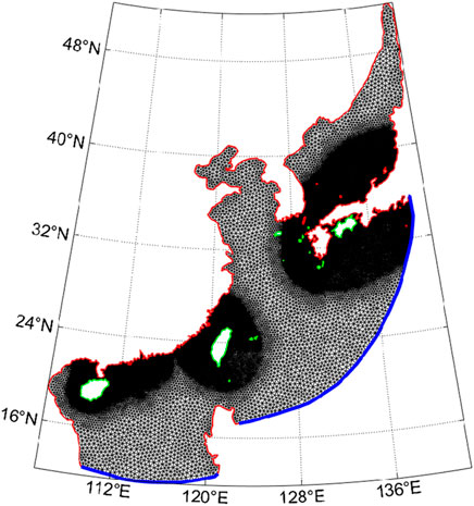
FIGURE 5. Unstructured mesh in the studying area.

The wave field of synthetic TC simulations was based on the SWAN model. The input of bathymetry was from the general bathymetric chart of the oceans (GEBCO) with its resolution of 0.5′×0.5′. The driven wind field was calculated by the model, which was explained in Section 3.2. The space resolution of the wind field and the resolution of time were 0.25° × 0.25° and 6 h, respectively. The time step and output were 30 min and every 6 h, respectively. The output parameters include significant wave height, wave direction, and average wave period.

4 Results

4.1 Typical tropical cyclone (TTC)

Figure 6 shows the six TTCs that were synthesized by the typical tracks and extreme intensity. The pentagram in the picture represents the strongest point in each type of TTC. TTC-I was formed in the east of the Philippines and moved to the northwest. It strengthened until the second landfall on Hainan Island and vanished in the Yunnan Province. The strengthening trend and direction of TTC-II were very similar to those of TTC-I. Its strongest point was at the position before its second landfall. It vanished in the Indochina Peninsula. TTC-III was the strongest and had the widest impact among the six TTCs, especially for the east of China. Its track traveled to the northwest first and gradually turned to the north after landfalling. Finally, it turned to the northeast. It strengthened to a peak to the east of the Taiwan Island before its landfall and then weakened. TTC-IV with a strong intensity had little impact on China because of its tracks. Its track recurved from northwest to southeast around 28 °N latitude and reached peak intensity before it landed in Japan. TTC-V and TTC-VI were formed in South China. They vanished in the Indochina Peninsula and Southwest of China, respectively. These two TTCs had a lower intensity and shorter lifespan. TTC-V impacted Hainan Island, whilst TTC-VI had little impact on China.

FIGURE 6

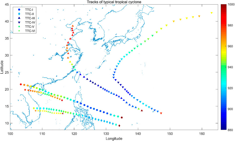
FIGURE 6. Synthesized typical tropical cyclones (TTCs).

Figure 7 shows the temporal P_c of 100 years, 1,000 years, and 10,000 years intensity for each type of TTC. Each P_c of TTC decreased to a minimum value that indicated the strongest intensity of TTC; then, it increased with time. The highest intensity was in TTC-III, followed by TTC-IV, TTC-I, TTC-II, TTC-V, and TTC-VI. Their values of P_c individually were 914 hPa, 924 hPa, 943 hPa, 957 hPa, and 970 hPa for 10,000 years occurrence, respectively.

FIGURE 7

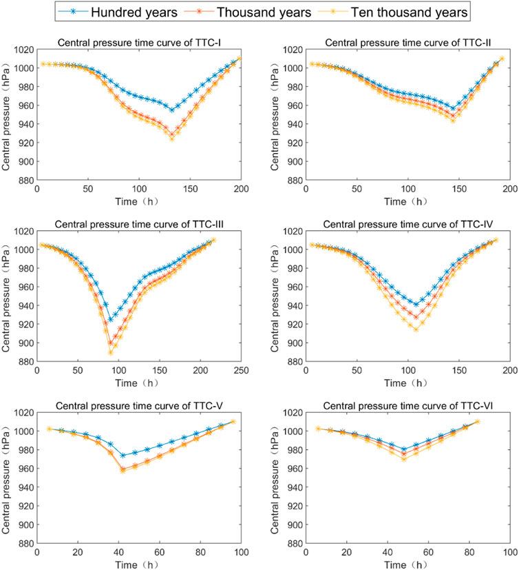
FIGURE 7. Temporal P_c of the recurrence period of 100, 1,000, and 10,000 years for each type of TTC.

4.2 Wind and wave model validations

To verify the model performance, four TCs of Bolaven, Mangkhut, Conson, and Mindule and two TCs of Kai Tak and Soulik were individually selected to validate the parametric wind model and the wave simulation model. The selected TCs and corresponding observation sites were individually listed and shown in Table 2 and Figure 8. The wind speed (W_s) and wind direction (W_d) curves calculated through the Holland wind model were compared with the observation data, as seen in Figure 9. The calibrated SWAN model was verified by using the wave data records. As shown in Figure 10, the time series of predicted significant wave heights (H_s) were well fitted with the measured data. To evaluate the quality of the verifications, the root mean square error (RMSE) and correlation coefficient (ρ) are listed in Table 3. The maximum RMSE, and the minimum values of ρ for wind speed and wind direction individually were 9.13, 0.81, and 0.93, respectively, indicating that both the wind and wave models performed well.

TABLE 2

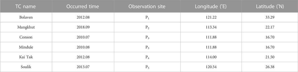
TABLE 2. Information on TCs and corresponding observation sites.

FIGURE 8

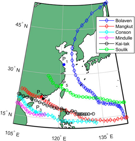
FIGURE 8. TCs and observation sites used to validate the wind and wave models.

FIGURE 9

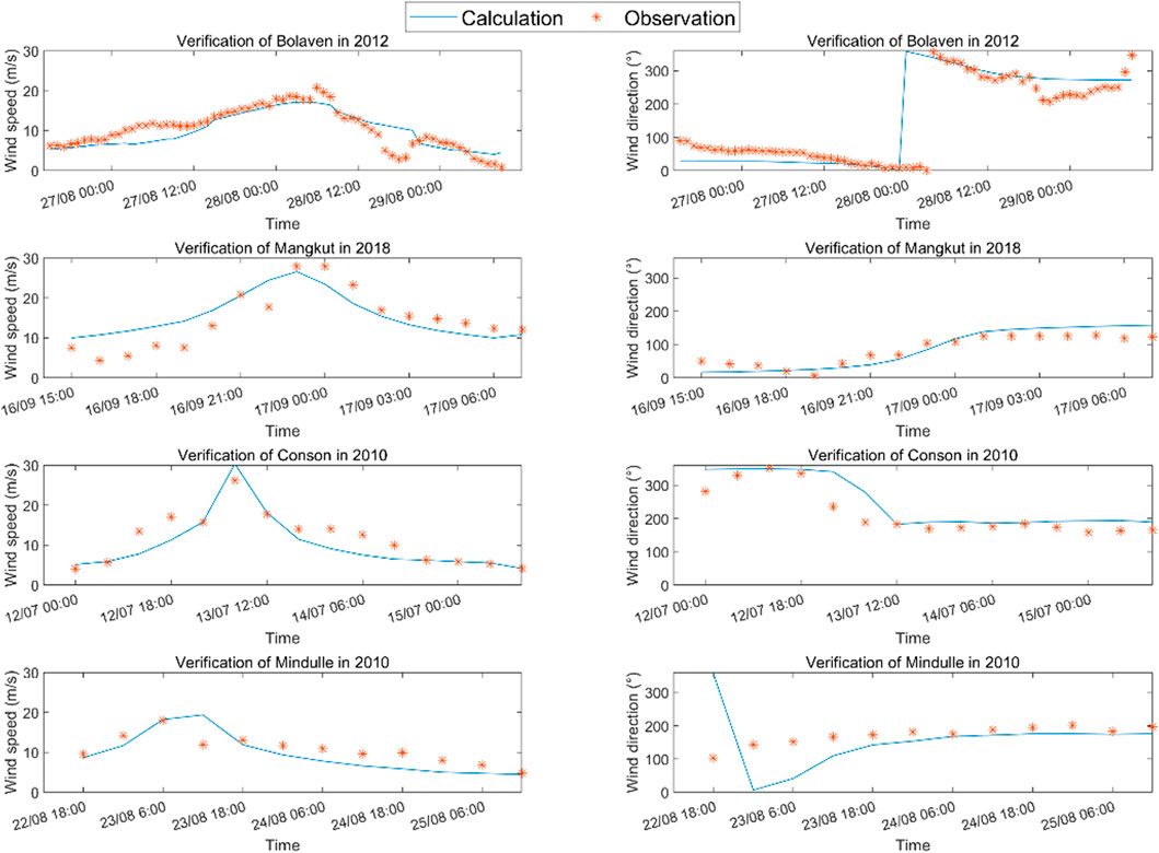
FIGURE 9. Wind speed and direction validations of Bolaven, Mangkhut, Conson, and Mindule.

FIGURE 10

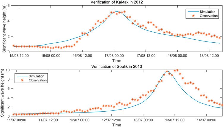
FIGURE 10. Significant wave height verification of Kai Tak and Soulik.

TABLE 3

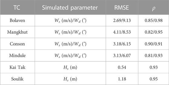
TABLE 3. Comparison analysis of wind and wave simulation results.

4.3 Wave field

The Holland model was used to calculate the wind field formed by TTCs. The wind fields of the six TTCs at their strongest moments for the recurrence period of 100, 1,000, and 10,000 years were shown in Figure 11. The first, second, and third columns individually represented the wind field forced by the TCs with the recurrence period of 100, 1,000, and 10,000 years. The first to sixth rows presented the TC types from TTC-I to TTC-VI. These rows and columns are the same in the following figures of Figures 12–14 as well. The color and the white arrows represent the magnitude of wind speed and wind direction, respectively. The wind speed near the typhoon center was the highest. The wind direction rotated counterclockwise around the typhoon center. Although it decreased gradually outward, the influenced areas were thousands of kilometers. Observing from the pictures, the longer the recurrence period, the greater the intensity and the wind speed. The maximum wind speed of TTC-III and TTC-IV was about 70 m/s, while those of TTC-I, TTC-II, TTC-V, and TTC-VI were about 60 m/s, 60 m/s, 50 m/s, and 50 m/s, respectively.

FIGURE 11

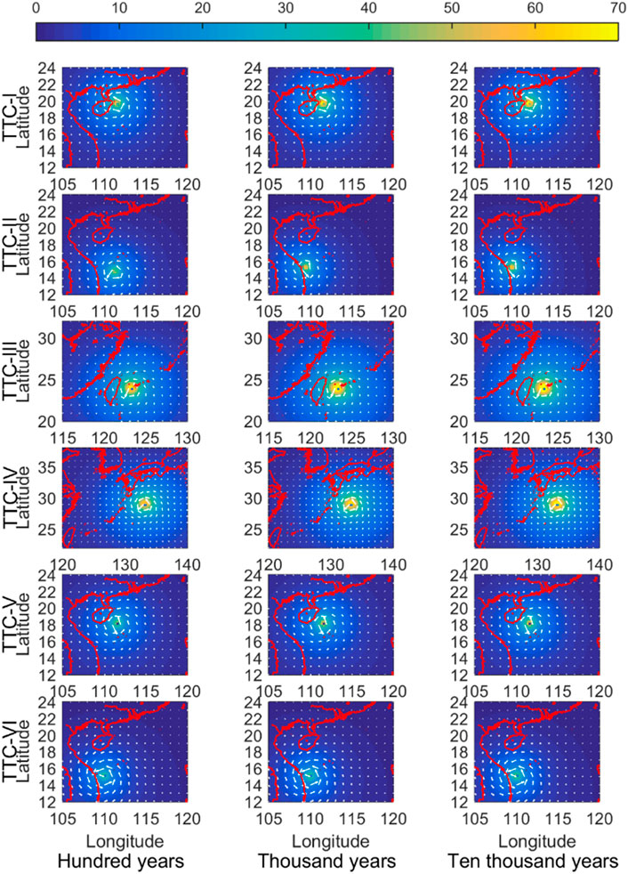
FIGURE 11. Wind field at the strongest moment of TTCs.

FIGURE 12

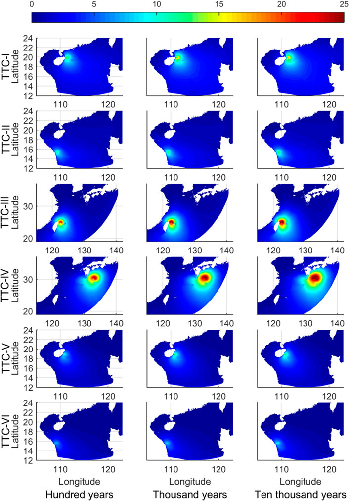
FIGURE 12. Spatial distributions of the simulated H_s at the strongest moment.

FIGURE 13

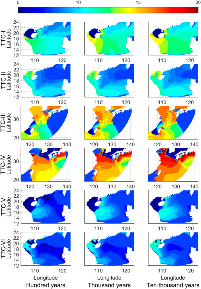
FIGURE 13. Spatial distributions of the peak period of the wave spectrum at the strongest moment.

FIGURE 14

FIGURE 14. Swaths of the maximum H_s formed by the TTC.

The wave field formed by the synthetic TC was simulated by the SWAN model. For the risk assessment and design standard, the extreme wave conditions for six typical TCs were considered in this study. The spatial distribution of the H_s simulation at the strongest moment during the TC process is shown in Figure 12, in which the columns and rows of the subfigure are the occurrence and types of TTCs. The maximum H_s values in each subfigure are listed in Table 4. Both TTC-III and TTC-IV generated the severest sea condition with H_s of about 30 m for the 10,000-year intensity. This was followed by TTC-I with 18 m H_s, and TTC-VI with the weakest, with less than 10 m H_s. The H_s formed by TTC-I and TTC-V reached their peaks when the typhoons approached landfall on Hainan Island.

TABLE 4

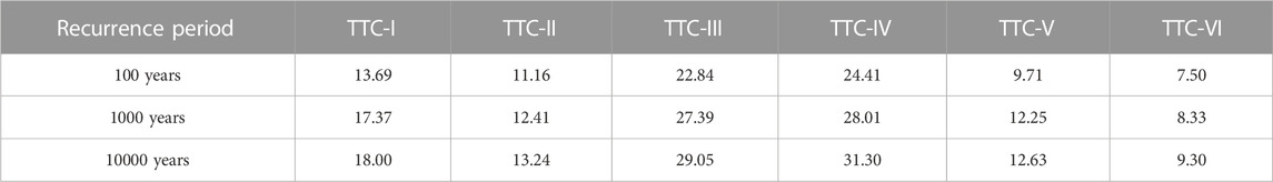
TABLE 4. Maximum H_s (unit: m) during the process in various TTCs and P_c values.

Figure 13 shows the spatial distributions of the peak period of the wave spectrum at the strongest moment. The columns and rows of the subfigure are the occurrence and types of TTC similar to those in Figure 11. The wave periods of TTC-III and TTC-IV were 15–17s, while those of the others were 8–11s.

The short-wave period occurred in the areas where the wave was in the growing stage. Figure 14 presents the swath variations from the spatial information on H_s in each TTC. The swaths were calculated by the largest H_s at each grid point during the TC process. The pictures indicated that the maximum H_s value moved forward along the TTC track. When TTC-I and TTC-V approached land, H_s increased. Specially, TTC-III and TTC-IV produced very large H_s all the time in the studied area. In contrast, TTC-II and TTC-VI generated a much weaker wave field, and thus, they had little effect on the nearshore sea state.

5 Discussion

5.1 The TC tracks

From the historical data, TC consisted of movers in curves and straights. If the turning flow changed direction, TCs moving westward would turn. TTC-III and TTC-IV represented this type of recurving TCs. TTC-III moved over land for a long time and would cause large damage, although its intensity was not very strong (Tuleya and Kurihara, 1978). Therefore, the TTC-III type should be given more attention. TTC-IVs that recurved over ocean represents TCs turning from northwest toward to the north and finally to the northeast without landfall on China. Since the regression rates are influenced by large-scale circulation patterns (Liu and Chan, 2003; Fudeyasu et al., 2006; Chen et al., 2009), the movement of TTC-I, TTC-II, TTC-V, and TTC-VI was relatively flat. Figure 15 shows the six types of TTC tracks and the position frequencies of the historical TC tracks, which are represented by black lines and colors. Each type of historical TC was concentrated in a certain place. The most frequent places that TTCs passed through indicated the representativeness of TTCs. TTC-I and TTC-V had the most probability of landfall on Hainan, Guangdong, and Guangxi provinces, while TTC-III landed on Taiwan, Fujian, and Zhejiang provinces and affected Jiangsu, Jiangxi, Anhui, Shandong, and Liaoning provinces. The Philippines and Japan were hit by TTC-I, TTC-II, and TTC-IV.

FIGURE 15

FIGURE 15. TTC tracks (the black lines) and the position frequency of historical TC tracks.

5.2 Intensity in spatial distribution

Although the TTC represents a type of TC, intensity distributions of TC may vary spatially. Figure 16 shows the spatial distribution of minimum P_c in the grid of 1° × 1° for each type of TC. The colors represent P_c values of TCs, and the lower the value, the higher the intensity. The track of TTC is drawn by the black line. The minimum P_c value was about 900 hPa near 20 °N, indicating that the intensity was strongest. Combining Figures 15, 16 together, there was a strong correlation between the position frequency and intensity. From the subplot (a) of Figure 16, if TTC-I orbited further north and crosses the Bashi Channel, the driven extreme wave may be larger than the present TTC-I. Due to the very low P_c off the eastern part of Hainan Island, severe sea conditions may occur in the nearshore areas. For TTC-II, TTC-III, and TTC-IV (Figures 16B–D), the severest sea states occurred in the southeast of Taiwan Island and east of the Philippines. For TTC-V and TTC-VI (Figures 16E, F), the TCs formed in the South China Sea had a weaker intensity compared to the other TTCs.

FIGURE 16

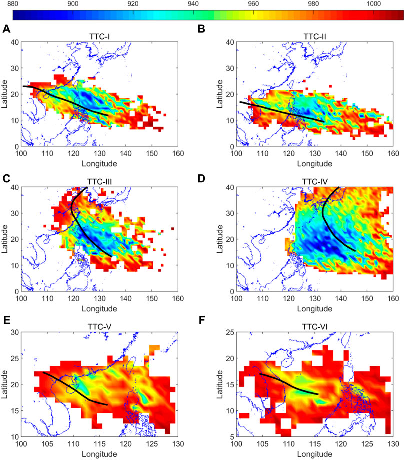
FIGURE 16. Spatial distributions of minimum P_c in the grid of 1° × 1° for each type of TC. (A) TTC-I; (B) TTC-II; (C) TTC-III; (D) TTC-IV; (E) TTC-V; (F) TTC-IV.

5.3 Comparisons with historical TCs

In order to further analyze the extreme representativeness of synthetic typical typhoons, four historical typhoons with high intensity, wide impact, and serious disaster-causing effects were selected. They were typhoon Haiyan in 2013, Typhoons Maria and Mangkhut in 2018, and typhoon Lekima in 2019. Both the tracks of the four typhoons and their time histories of central pressure are shown in Figure 17. Haiyan and Mankhut belong to Group I typhoons, while Maria and Lekima belong to Group III typhoons. Among these four typhoons, Lekima had the longest duration and the greatest impact on China, while Haiyan had the highest intensity.

FIGURE 17

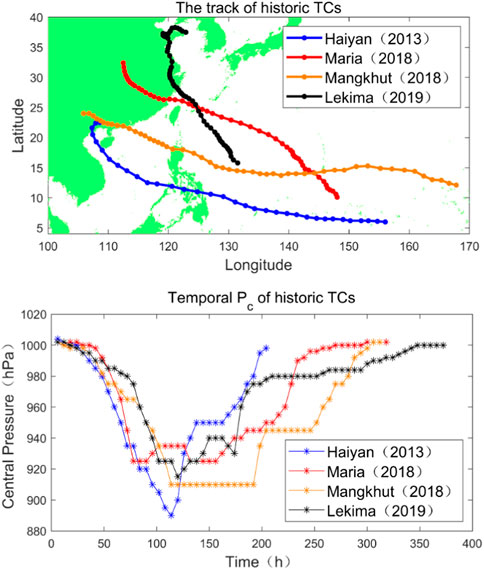
FIGURE 17. Track and temporal P_c of four historical TCs.

Similarly, the Holland parametric wind model was used to calculate the wind fields generated by the four historical typhoons as driving wind fields, and the SWAN model was used to simulate the wind and waves during the typhoon. Figure 18 shows the spatial distribution of the maximum significant wave heights produced by the four typhoons. The maximum significant wave height and minimum central pressure values caused by each typhoon are listed in Table 5. As seen from Figure 18 and Table 5, the wave height produced by Lekima was the largest, followed by those of Maria and Mangkhut, while the effective wave height produced by Haiyan was the smallest. However, the central pressure of Haiyan and Mangkhut was smaller and stronger. This was partly because the strongest points of Haiyan and Mangkhut were not in the study area and their intensity had been weakened after entering the South China Sea. In contrast to Haiyan and Mangkhut, Maria and Lekima were slightly weaker, but the significant wave height generated in this study area was larger. These could be analyzed from the track division, i.e., Haiyan and Mankhut belong to Group I typhoons, while Maria and Lekima belong to Group III typhoons. From the results in Subsection 4.3, Type-III typhoon produced relatively large effective wave heights. Therefore, the delineation of the location and the path of the strongest point of the typhoon were of great significance for typhoon intensity prediction and disaster analysis. Comparing the effective wave heights in Table 5 with those in Table 4, the recurrence period of Haiyan in Type-I was less than 100 years and that of Mangkhut was between 100 and 1,000 years. In type III, Maria occurs almost once every 100 years and Lekima occurs between 100 and 1,000 years.

FIGURE 18

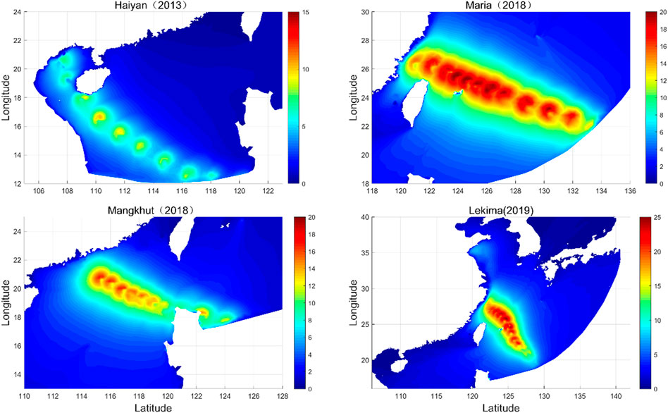
FIGURE 18. Maximum H_s interval formed by the four historical TCs.

TABLE 5

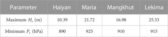
TABLE 5. List of the maximum H_s and the minimum P_c.

6 Conclusion

Extreme sea states induced by the super-strong TC will inevitably lead to marine disasters and large economic losses. Studying them is a paramount issue in risk assessment and marine disaster prevention. The TTC can help engineers anticipate the impact of an extreme TC at a certain site. In this paper, the wave fields driven by six synthetic TCs which have typical tracks and extreme intensity were analyzed. The significant wave height (H_s) and the peak period of the wave spectrum were also analyzed. The main conclusions are as follows:

TTC-I affects the north of the South China Sea and the coasts of Hainan, Guangdong, and Guangxi provinces and induces H_s as high as 18 m with a recurrence period of 10,000 years . TTC-II passes through the South China Sea with the highest H_s reaching 13.2 m with a 10,000-year recurrence period. The high intensity of TTC-III induces a 10,000-year recurrence period H_s of 29 m, threatening the East China Sea, Yellow Sea, and the eastern coastal cities of China. TTC-IV, which has a characteristic recurvature, represents the largest number of TCs. It influences Japan and eastern seas of China with a 10,000-year recurrence period H_s of 31.3 m. TTC-V influences the northern part of the South China Sea and the southern cities of China with its 10,000-year recurrence period H_s of 12.6 m. TTC-VI generates the weakest wave field and, thus, has little effect on the nearshore sea state.

Data availability statement

The original contributions presented in the study are included in the article/supplementary material; further inquiries can be directed to the corresponding author.

Author contributions

Conceptualization, SD; data curation, SD and ZY; formal analysis, SD and ZY; investigation, SD and ZY; methodology, SD and ZY; writing—original draft, SD; writing—review and editing, ZY.

Acknowledgments

The authors would like to acknowledge the support of the Ningbo Top Talents Program hosted by David Z. Zhu.

Conflict of interest

The authors declare that the research was conducted in the absence of any commercial or financial relationships that could be construed as a potential conflict of interest.

Publisher’s note

All claims expressed in this article are solely those of the authors and do not necessarily represent those of their affiliated organizations, or those of the publisher, the editors, and the reviewers. Any product that may be evaluated in this article, or claim that may be made by its manufacturer, is not guaranteed nor endorsed by the publisher.

References

Berg, R. (2016). Hurricane Hermine. National hurricane center tropical cyclone report. AL092016. 1–3. Available at: https://www.weather.gov/media/phi/StormReports/Hurricane_Hermine.pdf.

Google Scholar

Chen, T. C., Wang, S. Y., Yen, M. C., and Clark, A. J. (2009). Impact of the intraseasonal variability of the Western North Pacific large-scale circulation on tropical cyclone tracks. Weather Forecast. 24 (3), 646–666. doi:10.1175/2008WAF2222186.1

CrossRef Full Text | Google Scholar

Cox, D., Arikawa, T., Barbosa, A., Guannel, G., Inazu, D., Kennedy, A., et al. (2019). Hurricanes irma and Maria post-event survey in US Virgin Islands. Coast. Eng. J. 61 (2), 121–134. doi:10.1080/21664250.2018.1558920

CrossRef Full Text | Google Scholar

Fan, Y. L., Ginis, I., Hara, T., Wright, C. W., and Walsh, E. J. (2009). Numerical simulations and observations of surface wave fields under an extreme tropical cyclone. J. Phys. Oceanogr. 39 (9), 2097–2116. doi:10.1175/2009JPO4224.1

CrossRef Full Text | Google Scholar

Fan, Y. L., Lin, S. J., Held, I. M., Yu, Z. T., and Tolman, H. L. (2012). Global Ocean surface wave simulation using a coupled atmosphere-wave model. J. Clim. 25 (18), 6233–6252. doi:10.1175/JCLI-D-11-00621.1

CrossRef Full Text | Google Scholar

Fudeyasu, H., Iizuka, S., and Matsuura, T. (2006). Impact of ENSO on landfall characteristics of tropical cyclones over the Western North Pacific during the summer monsoon season. Geophys. Res. Lett. 33 (21), L21815. doi:10.1029/2006GL027449

CrossRef Full Text | Google Scholar

Graham, H. E. (1959). Meteorological considerations pertinent to standard project hurricane, Atlantic and Gulf Coasts of the United States. US Department of Commerce, Weather Bureau.

Google Scholar

Hasselmann, K., Barnett, T. P., Bouws, E., Carlson, H., Cartwright, D. E., Enke, K., et al. (1973). Measurements of wind-wave growth and swell decay during the joint north sea wave project (JONSWAP). Ergaenzungsheft zur Deutschen Hydrographischen Zeitschrift, Reihe A.

Google Scholar

Holland, G. J. (1980). An analytic model of the wind and pressure profiles in hurricanes. Mon. Weather Rev. 108 (8), 1212–1218. doi:10.1175/1520-0493(1980)108<1212:AAMOTW>2.0.CO;2

CrossRef Full Text | Google Scholar

Holland, G. J., Belanger, J. I., and Fritz, A. (2010). A revised model for radial profiles of hurricane winds. Mon. Weather Rev. 138 (12), 4393–4401. doi:10.1175/2010mwr3317.1

CrossRef Full Text | Google Scholar

Hong, J. S., Moon, J. H., Kim, T., and Lee, J. H. (2018). Impact of ocean–wave coupling on typhoon-induced waves and surge levels around the Korean Peninsula: A case study of typhoon bolaven. Ocean. Dyn. 68 (11), 1543–1557. doi:10.1007/s10236-018-1218-9

CrossRef Full Text | Google Scholar

Hsiao, S. C., Chen, H. E., Wu, H. L., Chen, W. B., Chang, C. H., Guo, W. D., et al. (2020). Numerical simulation of large wave heights from super typhoon nepartak (2016) in the eastern waters of taiwan. J. Mar. Sci. Eng. 8 (3), 217. doi:10.3390/jmse8030217

CrossRef Full Text | Google Scholar

Lalbeharry, R., Bigio, R., Thomas, B. R., and Wilson, L. (2009). Numerical simulation of extreme waves during the storm of 20–22 January 2000 using winds generated by the CMC weather prediction model. Atmosphere 47 (1), 99–122. doi:10.3137/oc292.2009

CrossRef Full Text | Google Scholar

Liu, K., and Chan, J. C. L. (2003). Climatological characteristics and seasonal forecasting of tropical cyclones making landfall along the South China coast. Mon. Weather Rev. 131 (8), 1650–1662. doi:10.1175//2554.1

CrossRef Full Text | Google Scholar

Mori, N., and Takemi, T. (2016). Impact assessment of coastal hazards due to future changes of tropical cyclones in the North Pacific Ocean. Weather Clim. Extrem. 11, 53–69. doi:10.1016/j.wace.2015.09.002

CrossRef Full Text | Google Scholar

Olfateh, M., Callaghan, D. P., Nielsen, P., and Baldock, T. E. (2017). Tropical cyclone wind field asymmetry—development and evaluation of a new parametric model. J. Geophys. Res. Oceans 122 (1), 458–469. doi:10.1002/2016JC012237

CrossRef Full Text | Google Scholar

Prakash, K. R., and Pant, V. (2020). On the wave-current interaction during the passage of a tropical cyclone in the Bay of Bengal. Deep-Sea Res. Part Ii-Topical Stud. Oceanogr. 172, 104658. doi:10.1016/j.dsr2.2019.104658

CrossRef Full Text | Google Scholar

Qiao, W., Song, J., He, H., and Li, F. (2019). Application of different wind field models and wave boundary layer model to typhoon waves numerical simulation in WAVEWATCH III model. Tellus A Dyn. Meteorology Oceanogr. 71 (1), 1657552–1657620. doi:10.1080/16000870.2019.1657552

CrossRef Full Text | Google Scholar

Roberts, K. J., and Pringle, W. J. (2018). OceanMesh2D: User guide―Precise distance-based two-dimensional automated mesh generation toolbox intended for coastal ocean/shallow water. United States: Computational Hydraulics Lab. University of Notre Dame. doi:10.13140/RG.2.2.21840.61446/2

CrossRef Full Text | Google Scholar

Rumpf, J., Weindl, H., Höppe, P., Rauch, E., and Schmidt, V. (2007). Stochastic modelling of tropical cyclone tracks. Math. Methods Operations Res. 66 (3), 475–490. doi:10.1007/s00186-007-0168-7

CrossRef Full Text | Google Scholar

Shao, Z., Liang, B., Li, H., Wu, G., and Wu, Z. (2018). Blended wind fields for wave modeling of tropical cyclones in the South China Sea and East China Sea. Appl. Ocean Res. 71, 20–33. doi:10.1016/j.apor.2017.11.012

CrossRef Full Text | Google Scholar

Shi, B. W., Yang, S. L., Temmerman, S., Bouma, T., Ysebaert, T., Wang, S., et al. (2021). Effect of typhoon-induced intertidal-flat erosion on dominant macrobenthic species (Meretrix meretrix). Limnol. Oceanogr. 66 (12), 4197–4209. doi:10.1002/lno.11953

CrossRef Full Text | Google Scholar

Tajima, Y., Yasuda, T., Pacheco, B. M., Cruz, E. C., Kawasaki, K., Nobuoka, H., et al. (2014). Initial report of jsce-pice joint survey on the storm surge disaster caused by typhoon haiyan. Coast. Eng. J. 56 (1), 1450006-1–1450006-12. doi:10.1142/S0578563414500065

CrossRef Full Text | Google Scholar

Tolman, H. L., Alves, J., and Chao, Y. Y. (2005). Operational forecasting of wind-generated waves by hurricane isabel at ncep. Weather Forecast. 20 (4), 544–557. doi:10.1175/waf852.1

CrossRef Full Text | Google Scholar

Tuleya, R. E., and Kurihara, Y. (1978). A numerical simulation of the landfall of tropical cyclones. J. Atmos. Sci. 35 (2), 242–257. doi:10.1175/1520-0469(1978)035<0242:ANSOTL>2.0.CO;2

CrossRef Full Text | Google Scholar

Umesh, P. A., and Behera, M. R. (2020). Performance evaluation of input-dissipation parameterizations in WAVEWATCH III and comparison of wave hindcast with nested WAVEWATCH III-SWAN in the Indian Seas. Ocean. Eng. 202, 106959. doi:10.1016/j.oceaneng.2020.106959

CrossRef Full Text | Google Scholar

Umesh, P. A., and Swain, J. (2018). Inter-comparisons of SWAN hindcasts using boundary conditions from WAM and WWIII for northwest and northeast coasts of India. Ocean. Eng. 156, 523–549. doi:10.1016/j.oceaneng.2018.03.029

CrossRef Full Text | Google Scholar

Wang, D. W., Mitchell, D. A., Teague, W. J., Jarosz, E., and Hulbert, M. S. (2005). Extreme waves under hurricane ivan. Science 309 (5736), 896. doi:10.1126/science.1112509

PubMed Abstract | CrossRef Full Text | Google Scholar

Wu, G., Shi, F., Kirby, J. T., Liang, B., and Shi, J. (2018). Modeling wave effects on storm surge and coastal inundation. Coast. Eng. 140, 371–382. doi:10.1016/j.coastaleng.2018.08.011

CrossRef Full Text | Google Scholar

Wu, G. X., Wang, J., Liang, B. C., and Lee, D. Y. (2014). Simulation of detailed wave motions and coastal hazards. J. Coast. Res. 72, 127–132. doi:10.2112/SI72-024.1

CrossRef Full Text | Google Scholar

Wu, Z. Y., Jiang, C. B., Deng, B., Chen, J., Cao, Y. G., and Li, L. J. (2018). Evaluation of numerical wave model for typhoon wave simulation in South China Sea. Water Sci. Eng. 11 (3), 229–235. doi:10.1016/j.wse.2018.09.001

CrossRef Full Text | Google Scholar

Xu, Y., He, H., Song, J., Hou, Y., and Li, F. (2017). Observations and modeling of typhoon waves in the South China sea. J. Phys. Oceanogr. 47 (6), 1307–1324. doi:10.1175/JPO-D-16-0174.1

CrossRef Full Text | Google Scholar

Xu, Y., Zhang, J. C., Xu, Y., Ying, W. M., Wang, Y. P., Che, Z. M., et al. (2020). Analysis of the spatial and temporal sensitivities of key parameters in the SWAN model: An example using Chan-hom typhoon waves. Estuar. Coast. Shelf Sci. 232 (5), 106489. doi:10.1016/j.ecss.2019.106489

CrossRef Full Text | Google Scholar

Yan, Z., Liang, B., Wu, G., Wang, S., and Li, P. (2020). Ultra-long return level estimation of extreme wind speed based on the deductive method. Ocean. Eng. 197, 106900. doi:10.1016/j.oceaneng.2019.106900

CrossRef Full Text | Google Scholar

Yang, S. L., Fan, J. Q., Shi, B. W., Bouma, T. J., Xu, K. H., Yang, H. F., et al. (2019). Remote impacts of typhoons on the hydrodynamics, sediment transport and bed stability of an intertidal wetland in the Yangtze Delta. J. Hydrology 575, 755–766. doi:10.1016/j.jhydrol.2019.05.077

CrossRef Full Text | Google Scholar

Yasuda, T., Nakajo, S., Kim, S., Mase, H., Mori, N., and Horsburgh, K. (2014). Evaluation of future storm surge risk in East Asia based on state-of-the-art climate change projection. Coast. Eng. 83, 65–71. doi:10.1016/j.coastaleng.2013.10.003

CrossRef Full Text | Google Scholar

Ying, M., Zhang, W., Yu, H., Lu, X., Feng, J., Fan, Y., et al. (2014). An overview of the China Meteorological Administration tropical cyclone database. J. Atmos. Ocean. Technol. 31 (2), 287–301. doi:10.1175/JTECH-D-12-00119.1

CrossRef Full Text | Google Scholar

Zijlema, M. (2010). Computation of wind-wave spectra in coastal waters with SWAN on unstructured grids. Coast. Eng. 57 (3), 267–277. doi:10.1016/j.coastaleng.2009.10.011

CrossRef Full Text | Google Scholar