- School of Environmental Sciences, Jawaharlal Nehru University, New Delhi, India
Urban heat islands (UHI) are developing due to increasing urbanization and loss of vegetation in major cities in India. Increased urbanization modifies the urban microclimate that leads to significant land-use changes resulting in surface conversion and heat release, which poses serious risks to human health, environment and the ecosystem of the Himalayan ecosystem. Hence, mitigating UHI becomes important and requires a better understanding of underlying associated biophysical processes. In the study an attempt has been made to demonstrate the impact of urbanization on land surface temperature (LST) in Shimla and Dehradun, capitals of the Western Himalayan states, India using satellite data and spatial metrics. The process was analyzed using urban coverage patterns obtained from Landsat 5, 7, and 8 and corresponding sensors from TM, ETM+, and OLI. The Built-up and Non-Built-up areas were extracted and the biophysical parameters NDVI, NDBI, NDWI and LST were calculated to capture different features of urban growth. The result indicated, that the built-up area increased from 32.19 km2 (2000) to 68.37 km2 (2016) in Dehradun and from 12.38 km2 (2000) to 29.47 km2 (2016) in Shimla during the study period, resulting in an increase in NDBI and LST and Reduction and NDVI and NDWI. Results showed that temperature hotspots were largest in urban areas, followed by vegetation and water bodies. A significant correlation (p < 0.05) was observed between LST and biophysical parameters -NDVI, NDBI, NDWI. Spatial metrics at the class and landscape levels show that increased urban growth from 2000 to 2016 has made the landscape fragmented and more heterogeneous. The Identified trends and changes in landscape patterns and their impact on heterogeneous urban areas suggest that the study is feasible to estimate LST, NDVI, NDBI and NDWI with reasonable accuracy that will likely have influence on policy interventions.
1 Introduction
An increase in surface temperature on account of the reduction in vegetated surface and its conversion into impervious surfaces in urban areas is one of the most pressing issues cities confront nowadays (Mallick et al., 2008). These changes affect numerous aspects of cities, including land use, transportation, infrastructure and the environment (Weng et al., 2004; Mallick et al., 2008). Urbanization being a global process and is occurring at an escalating rate in developing countries and continuously modifying the land use pattern (Sharma and Joshi, 2012). Increased urbanization contributes to environmental degradation, one of the primary drivers of climate change (Chen et al., 2006; McCarthy et al., 2010). Large-scale urbanization has a distorting effect on the climate in cities and the areas around them (Liu et al., 2018). Conversion of vegetated surfaces to urban land use categories and urban areas experienced an increase in surface temperature and on the verge of developing urban heat islands (Giridharan et al., 2004; Neteler, 2010; Ogashawara and Bastos, 2012; Grover and Singh, 2015).
An important factor in comprehending the land-surface process at both the regional and global scales is the land surface temperature (LST), which serves as a primary indication of the Earth’s energy balance (Dewan et al., 2009; Peng et al., 2018). LST is influenced by vegetation and the amount of water in the soil, which provide important information about how numerous environmental systems are operating (Weng et al., 2004; Rashid et al., 2022). Using meteorological data to predict long-term land surface temperature (LST) change is challenging because of the insufficient and sparse availability of meteorological stations in these regions (Zhou et al., 2019). Remote sensing has proved to be one of the vital technologies for providing valuable information such as temporal land cover change analysis and risk analysis at various scales (Punia and Singh, 2012; Guha et al., 2020) and modeling the urban growth patterns (Bhatta, 2009). Satellite images are frequently utilizing to investigate the rate and scope of urbanization on a global and regional scale (Keles et al., 2007; Mishra et al., 2020; Ashwini and Sil, 2022). It provides more detailed view of the human landscape (Carlson, 2003) when superimposed on demographic or geographic data (Joshi et al., 2001; Roy and Tomar, 2001; Rawat and Kumar, 2015).
Several researches have been conducted on assessing the urban built-up and the relationship of NDVI, NDWI, NDBI on LST in foreign nations. There have not been many studies done in India, and those that have been done have primarily focused on megacities like Delhi (Mallick et al., 2013), Mumbai (Grover and Singh, 2015), Chennai (Lilly Rose and Devadas, 2009), Jaipur (Jalan and Sharma, 2014), Bangalore (Ramachandra et al., 2012b), and Hyderabad (Wakode et al., 2014). In the Himalayan foothills, new urban areas are growing at the expense of agricultural and forested land, changing the region’s environment (Munsi et al., 2009). However, a few studies have been conducted for cities in the Himalayan region that determined the degree of relationship between water, vegetation, and built-up areas on LST (Kuldeep and Kamlesh, 2011; Pal and Ziaul, 2017). These human activities have resulted into modification of the environment and consequent habitat loss and fragmentation of landscape (Midha et al., 2010). The anthropogenically caused urban development patterns and their effects on forest health are characterized by means of landscape metrics (Munsi et al., 2010; Srinivasan et al., 2022). Many scholars have used landscape spatial analysis in conjunction with geographic information systems as a useful method for tracking urban planning and growth (Pham and Yamaguchi, 2011; Triantakonstantis and Stathakis, 2015; Annes et al., 2018).
Therefore, it’s become critical to minimize the rise in land surface temperature and consequent emergence of UHI through monitoring and implementing appropriate land-use plans. In view of this, the present study examines the relationship between surface biophysical parameters and surface temperature variation (LST) which have occurred in the mountain regions in the past few decades, and also to estimate the role played by the urbanization on LST in space and time. The study is primarily focused on the dynamics of urban growth using Landsat TM, ETM, OLI satellite data and spatial metrics for two Indian Himalayan cities Dehradun and Shimla from 2000 to 2016. These two cities have witness drastic changes in land use categories primarily on account of increased built-up areas, conversion of agriculture and forest land, and economic developmental projects in the last 2–3 decades. Moreover, we assessed how vegetation (NDVI), Hydrology (NDWI) and Built-up (NDBI) have an impact on LST. Spatial and temporal fragmentation of these two cities have also been studied using landscape metrics to quantify the structure of the landscape. The findings of this study may prove beneficial for city planners and policymakers for the sustainable management of these two Himalayan cities.
2 Material and methodology
2.1 Study area
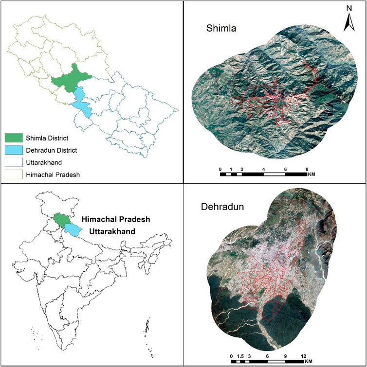
Dehradun, the capital of Uttarakhand, is 450 m above sea level and situated in the Doon valley in the Garhwal region of northern India between the latitudes of 29°58′N and 31°2′N and 77°34′E and 78°18′E. (Figure 1). The area is home to important national parks and wildlife refuges such Rajaji National Park, Benog Wildlife Sanctuary, and Asan Conservation Reserve. It falls within the category of a humid subtropical climate. While the average winter temperature ranges from 1–20°C, the summer temperature can reach 44°C for a few days. Dehradun had 1,696,694 residents in 2011 according to the census conducted in India (http://censusindia.gov.in). The state of Himachal Pradesh in northern India, which is situated in the foothills of the Himalayas, has Shimla as its capital. Seven distinct hills in total comprise Shimla and is located between 31.61 N and 77.10 E. The district, which is located at an elevation of 2206 m and is surrounded by Mandi, Kullu, Kinnaur, and Uttarakhand state (Figure 1). According to the Koppen’s climate classification, it has a subtropical highland climate. In the summer, the average temperature ranges from 19°C–28°C, and in the winter, it ranges from −1–10°C. Shimla city had an estimated 814,010 residents as per the 2011 India census (http://censusindia.gov.in). The two cities being states capitals and also a tourist place have undergone remarkable changes in land use categories resulting into conversion of forested and agriculture lands into built-up areas. This necessitated having a scientific understanding of current land use categories so as to formulate proper policy framework for sustainable management of the two Himalayan cities.
2.2 Acquisition of satellite data
The United States Geological Survey (USGS) Earth Explorer (http://earthexplorer.usgs.gov/) was used to collect data for the Landsat series satellites over a 16-year period (2000–2016). Table 1 lists the path/row and other characteristics of the satellite data. Landsat data were chosen because of their wider availability in the public domain-spatially and temporally at medium resolution besides containing thermal bands that were used in calculating land surface temperature to understand urban dynamics and thermal behavior of the environment focusing on surface physical characteristics in the form of temperature. Google Earth images were additionally employed in the study for visual interpretation and confirmation.
2.3 Image processing
Satellite data when taken has some form of errors associated with it. This error should be removed by using appropriate algorithms for scene matching and change detection analysis. Satellite data pre-processing include atmospheric correction, geometric correction, and radiometric correction. The acquired data were geometrically and atmospherically corrected and layer stacked using ERDAS IMAGINE 9.1. The boundary layer of Shimla and Dehradun city was procured and a buffer of 5 km was created and clipped for each image from their respective stacked images using the Arc GIS 10.3. Later on and false color composite (FCC) images were created. All the clipped images were classified using the unsupervised nearest neighborhood classification technique wherein the software disparate a large number of obscure pixels based on the reflectance values into classes without direction from the user (Tou Gonzalez, 1974). The statistical groupings in the data were controlled by a clustering algorithms application. Each image was divided into five classes: forest, agriculture, open land, water body, and urban area. The classified images were afterwards adjusted with Google Earth, recoded with the ERDAS recode option, and then divided into two classes, Built-up and Non-Built up areas. According to the following equations, biophysical parameters including LST, NDVI, NDWI, and NDBI as well as spatial matrices were calculated.
2.4 Calculation of LST from thermal bands
2.4.1 Conversion from DN to spectral radiance (
Every object above absolute zero (K), emits electromagnetic radiation in the form of Thermal Energy. Spectral radiance was calculated using Eq. 1 (Landsat Project Science Office, 2002; Chander et al., 2009).
where, Gain = Slope of radiance/DN conversion function,
2.4.2 Conversion of radiance to top of atmosphere reflectance (TOA)
The depletion in between-scene variability was achieved by the normalization process for solar irradiance by changing spectral radiance to the top of atmosphere reflectance. The combined surface and atmospheric reflectance of the image was calculated following Eq. 2 (Chander et al., 2009).
where,
2.4.3 Calculation of at-sensor brightness
The effective at-sensor brightness temperature (Tb) also known as black body temperature was derived from the spectral radiance using Plank’s inverse function. At-sensor brightness temperature under the assumption of uniform emissivity was calculated following (Weng and Lu, 2008).
Where,
2.4.4 Calculation of NDVI
For calculation of LST, emissivity corrected images were required which were calculated using a modified NDVI threshold method using Eq. 4 (Sobrino et al., 2004).
where, λNIR = Wavelength of NIR band (band 4 of TM and ETM + and OLI band 5) and λRED = Wavelength of Red band (band 3 of TM and ETM + and OLI band 4)
Values between 0 and 1 indicate vegetation cover, nearer to 1 indicate higher vegetation density.
2.4.5 Emissivity correction
The temperature readings from above are expressed in terms of a black body. As a result, spectral emissivity (ε) modifications were required based on the kind of land cover. The thermal band data was transformed from effective at-sensor brightness temperature to at-sensor spectral radiance. Therefore, emissivity effects are taken into account if the Earth’s surface is a blackbody and includes air effects (absorption and emission along the path). The method for emissivity adjustment that is most frequently employed is the NDVI threshold method. Using a spatial model maker in the ERDAS, the NDVI generated pictures were applied for the emissivity adjustment.
2.4.6 Calculation of LST from emissivity
The land surface temperature was calculated using Eq. 5 (Artis and Carnahan., 1982)
where, Tb = Brightness temperature, ε = Final Emissivity, λ = Effective wavelength, σ = Boltzmann constant (1.38*10−23 J/K), h = Plank’s constant (6.626*10−24Js) and c = velocity of light in vacuum (2.998*108 m/s).
Finally, to comprehend easily, the derived LST was converted to °C using the relation 0°C = 273.15 K.
2.5 Normalized difference built-up index (NDBI)
NDBI automatically maps built-up features of urban areas which were computed following the method devised by Zha et al., 2003). The method takes advantage of the spectral feature of built-up areas and other land covers (He et al., 2010).
Where,
2.6 Normalize difference water index (NDWI)
NDWI is an index that estimates the moisture content of the vegetation canopy. It uses two NIR channels (Gao et al., 1996). It provides important information regarding the conversion of a vegetated area to a non-vegetated area.
Where,
2.7 Degree of association between NDBI, NDVI, NDWI and LST
More than 100 points from the LST image were randomly picked, and the NDVI, NDBI, and NDWI values associated with those points were calculated in order to assess the association between LST and these metrics. Analysis of correlations between LST values and each biophysical parameter’s related values was done. Additionally, regression analysis for NDVI, NDBI, and NDWI was performed to determine how variations in land-use intensity through time and space affect LST.
2.8 Spatial metrics analysis
Spatial metrics are a crucial tool for measuring and quantifying urban sprawl (Herold et al., 2005) and have been used to explicitly capture spatial variation and the morphological aspects of urban formations (Herold et al., 2003; Prastakos et al., 2012). It is a spatial pattern analysis application for quantifying landscape structure, created for category maps to work with geospatial data and assist the user in categorizing landscape patterns and metrics as well as identifying the region where land use activities have led to fragmentation (Martin Balej, 2012). At the patch, class, and landscape levels in landscape ecology, spatial metrics measures offer valuable numerical descriptions (Yu and Ng, 2006; Martin Balej, 2012; McGarial, 2013). Utilizing FRAGSTATS 4.2 (McGarial and Mark, 1995), landscape metrics were computed at the landscape and class level to better understand the factors influencing urban transitions. Altogether six metrics were used for landscape-level (Table 2) namely Total Edge (TE), Edge density (ED), Shape Index (SHAPE), Shannon’s index (SHDI) (Shannon and Weaver, 1949), Simpson’s index (SIDI), Simpson’s Evenness Index (SIEI) and five metrics at class level namely Contiguity Index (CONTIG), Perimeter area ratio (PARA), Edge density (ED), Total Edge (TE) and shape index (SHAPE) are computed to know land-use changes which can be correlated with the degree of urbanization (Dasgupta et al., 2009). The specified parameters are helpful in locating the primary factors that represent urban dynamics. Edge density (ED) is the length of the edge per unit area. The best way to think of edge metrics is as a representation of the landscape. CONTID is used to create the landscape aggregate (Herold et al., 2002). The total number of edges in a landscape is correlated with its level of spatial variability. The shape index (SI) measures the complexity of the patch shape with a standard shape. Landscape composition is quantified through diversity measures. SHDI, SIDI and SIEI were computed to understand the fragmentation because of urban sprawl (Joshi et al., 2006; Fenta et al., 2017). Simpson’s index gives the likelihood that any two patches when selected at random will be of different types. The higher the SIDI value, the greater would be the diversity.
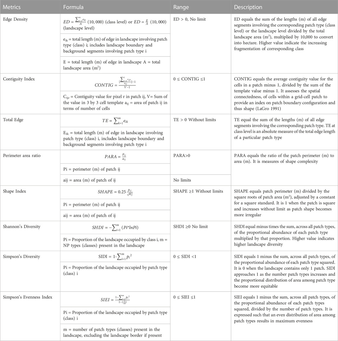
TABLE 2. Details of class and landscape level metrics used in the study, following (McGarigal, 2015).
2.9 Method adopted for validation
500 testing points that were uniformly dispersed over the whole region of interest chosen at random and used to evaluate the accuracy of the data. These measurement locations points were employed for each time period, NDBI, NDVI, NDWI, built-up and non-built-up conditions. A field survey and Google Earth were used as the foundation for the validation. We estimated overall accuracy (Story and Congalton, 1986) for validation as we had two classes to validate. The overall accuracy was computed as overall accuracy (%) = Number of correct samples/total samples × 100% (Congalton and Green, 1999). Based on the meteorological station data obtained from the World Meteorological Station Climate Explorer data (https://climexp.knmi.nl/start.cgi), the Land Surface Temperature Model for both Dehradun and Shimla was validated. The daily temperature data was selected for October and November for the years 2000, 2008 and 2016 and compared against the mean temperature derived from the land surface temperature model. The LST model was also verified from the climate research unit (CRU) time series high resolution (0.5° × 0.5°) gridded temperature datasets (Harris et al., 2020). The monthly temperature data from the CRU was retrieved for the respective month and year of satellite data collection and compared against the mean LST model derived temperature.
3 Result and discussion
3.1 Land cover change analysis
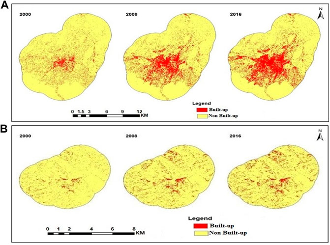
Considering the interest of the study two classes i.e. built-up and Non-built up have been generated for the two cities. Dehradun has ascribed the conversion of non-urban regions including forests, grasslands, fallow land, and agricultural land to built-up areas over a sixteen-year period to an increase in population (Figure 2A). The area that was considered to be urbanized in 2000 was 32.19 km2, and that area expanded to 55.94 km2 in 2008 and then to 68.37 km2 in 2016. In the city’s center, the built-up area became more concentrated. The sprawl surrounding the city’s center continued in 2008 and reached the outside of the city limits. Urban areas clearly grew between 2000 and 2008, which is linked to the rise in population. However, in 2016 both the central city and the surrounding areas saw a concentration of urban expansion. The center of the city now has a higher concentration of built-up areas. Shimla’s urban sprawl map divides the area into two categories: built-up and non-built-up (Figure 2B). The built-up area underwent a leapfrogging effect between 2000 and 2008, which indicates a quick transformation. The pattern of urbanization has become more dispersed and less concentrated throughout the central area. Urbanization was calculated for an area of 12.38 km2 in 2000. By 2008, that area had nearly doubled to 23.63 km2, and by 2016, it had grown even more to 29.47 km2. Several studies in the Himalaya highlighted similar changes in land use land cover changes by Gautam et al. (2002); Mishra et al. (2020); Ashwini and Sil, (2022). Bhatt et al. (2017) have also found significant land use changes to urban area during 2004–2014 in the Dehradun city resulting in sharp decline in agriculture, fallow and vacant land.
Based on a random selection of 500 testing points for each city and time period, the accuracy of the classified images, LST, and other biophysical parameters such as NDVI, NDBI, and NDWI were verified and compared. Overall accuracy was determined to be 93.2% (2000), 94.8% (2008), and 96.7% (2016) for Dehradun and Shimla, respectively, and to be 95% (2000), 96.6% (2008), and 97% (2016) for Dehradun. Overall NDVI accuracy was found to be 92.72% (2000), 94.72% (2008), and 95.81% (2016) for Dehradun, and 95.2% (2000), 93.4% (2008), and 92.2% (2016) for Shimla. In terms of overall accuracy, NDBI was reported to be 91.81% in 2000, 96.18% in 2008, and 95.27% in 2016. For Shimla, it was 96% in 2000, 94.4% in 2008, and 94.2% in 2016. The NDWI accuracy for Dehradun was 95.81% (2000), 96.72% (2008), and 96.54% (2016), and that it was 92.8% (2000), 92.4% (2008), and 93.6% (2016) for Shimla. The accuracy of the classified map shows increasing trend over time for both the cities possibly because of the availability of higher resolution imageries in recent times. The Pearson’s correlation between the temperature deduced from LST and the daily temperature data for October and November was calculated for LST validation and assessed at the 0.01 level of significance. Dehradun’s correlation coefficient values were determined to be 0.4602, 0.562, and 0.634 in 2000, 2008, and 2016 correspondingly, while Shimla’s values were 0.485, 0.62, and 0.586 in those same years. At the 0.01 level, each of these values was significant. Additionally, a 2–4°C temperature disparity was noted between the LST model and meteorological station temperature. Additionally, it was discovered that the monthly temperature obtained from gridded climatic records varied by 3–6°C. It can be inferred that LST-derived temperature is reliable as a result of these strong correlations.
3.2 Degree of association of different biophysical parameters with LST
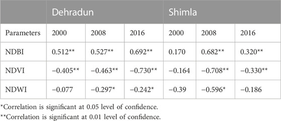
The association between LST and various biophysical factors (Table 3) was examined in order to statistically characterize the variation in LST. At 5% and 1% confidence levels, the Pearson’s correlation values were considered significant. The built-up areas have the most influence over LST, according to the correlation coefficient (R) between various LST deriving factors and LST (R of LST vs. NDBI ranges from 0.57 to 0.69 for Dehradun and from 0.17 to 0.68 for Shimla), followed by water bodies (R of LST vs. NDWI ranges from −0.07 to −0.29 for Dehradun and from −0.17 to −0.68 (R of LST vs. NDVI range from −0.45 to −0.73 for Dehradun and from −0.1 to −0.70 for Shimla). Therefore, it is clear that the LST is positively connected with NDBI and negatively correlated with NDVI and NDWI. As a result, greater land surface temperatures are observed in places with less vegetation and water, whereas higher built-up areas suffer lower LST.
3.3 Change in land surface temperature (LST)
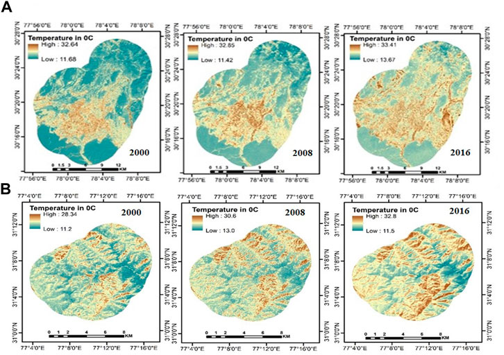
The regional distribution of the surface temperature in Dehradun is depicted in Figure 3A. The LST for Dehradun varies from 11.68°C to 32.64°C in 2000 (mean 23.68°C and SD 1.58), 11.42°C–32.85°C in 2008 (mean 26.49°C and SD 4.26) and 13.67°C–33.41°C in 2016 (mean 24.54°C and SD 1.16). According to Figure 3B, the temperature in Shimla ranged from 11.2°C to 28.34°C (mean 33.67°C and SD 5.80) in 2000, 13.0°C–30.6°C (mean 32.31°C and SD 4.74) in 2008, and 11.5°C–32.8°C (mean 24.78°C and SD 2.49) in 2016. It has been noted that the central region has high temperatures, which may be related to the area’s dense urbanization, while the forested regions saw moderate temperatures. The radiant temperature is lowered by natural plants or forests because they decrease the amount of heat that is absorbed into the soil through evapotranspiration. Shimla has seen similar patterns as more and more forested areas are turned into urban areas, which has led to an increase in temperature. LST is impacted by a variety of other factors in addition to changes in land use, which together cause changes in LST. These factors are natural and human. Natural factors that influence the LST include changes in the local hydrological cycle, global climate change, and a wide range of others. In terms anthropogenic, population growth has been a significant factor in addition to economic activities. In the past 2 decades, the population of the Dehradun and Shimla has multiplied, increasing both the urban population and urban clusters.
3.4 Association of NDBI with LST
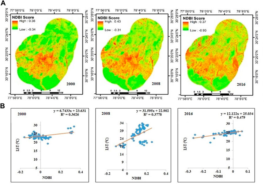
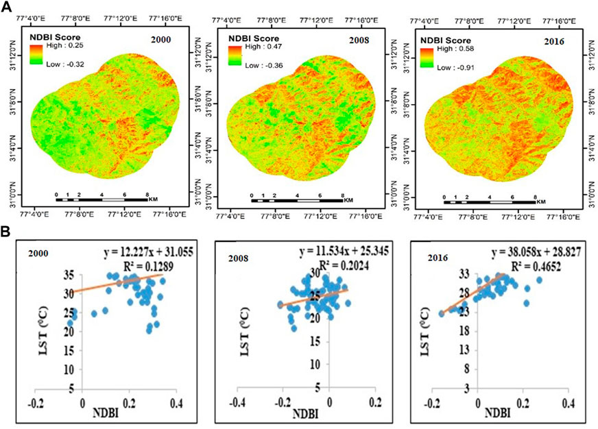
Figures 4A, 5A in the NDBI classifications for Dehradun and Shimla, respectively, demonstrate the spatial distribution and intensity of urban areas for the years 2000, 2008, and 2016, respectively. Both the spatial extent and intensity of urbanization were reported to have increased temporally. The patterns shown supported the findings that urbanized areas retain the most LST. Similar results were determined by Weng and Yang (2004) wherein they argued that less vegetation covers leads to increased LST. Xiao and Weng, 2007 have also reported that built-up area positively correlates with land surface temperature in Beijing, China.
The obtained coefficient of determination (R2) for Dehradun was R2 = 0.26 in 2000, increased to R2 = 0.27 in 2008, and further increased to R2 = 0.47 in 2016. Linear regression models between the NDBI and LST were fitted (Figure 4B). Similar trends were seen in Shimla, where the R2 value in 2000 was R2 = 0.02 and grew to R2 = 0.10 in 2008 and then to R2 = 0.46 in 2016 (Figure 5B). According to the coefficient of determination, LST and NDBI scores positively influenced each other over the study period.
3.5 Association of NDVI with LST
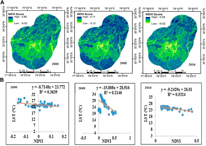
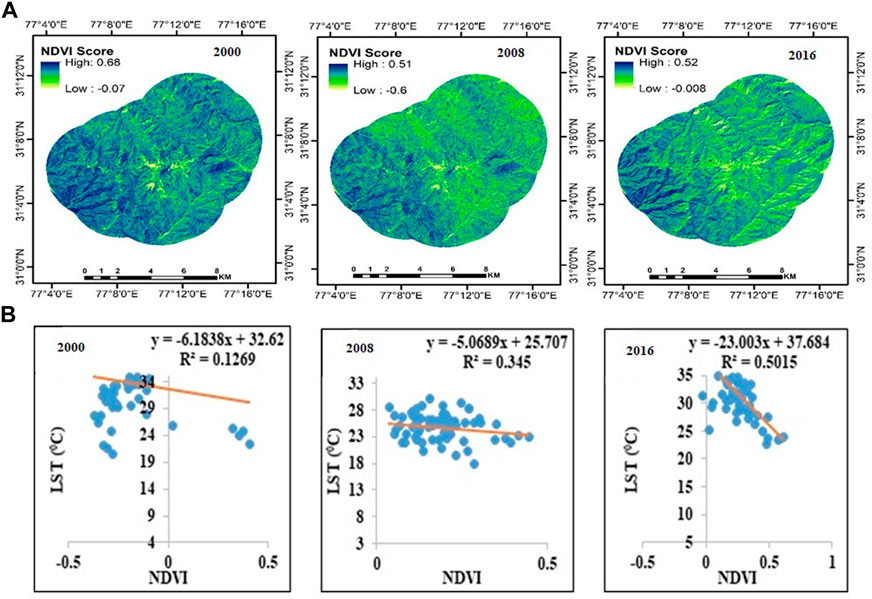
NDVI was utilized to distinguish between vegetated and non-vegetated areas in order to characterize the effect of changes in land cover on temperature trends. For Dehradun (Figure 6A) and Shimla, the geographical pattern and distribution of NDVI computed from Landsat images are displayed in Figure 7A. The NDVI measurements for Dehradun were found to range from −0.52 to 0.80 for 2000, with a mean of 0.00959 and a standard deviation of 0.0738; from −0.12 to 0.71 for 2008; from 0.1534 and 0.1356; and from −0.02 to 0.58 for 2016, with a mean of 0.1584 and a standard deviation of 0.0921. A low NDVI value (Yellowish area) indicates high and densely populated areas, mostly in the city’s central region, which increased steadily between 2008 and 2016. High NDVI values (dark blue) are seen close to the buffer area’s edge. On the outskirts of Dehradun, medium NDVI values (yellowish blue) are seen. The NDVI values for Shimla were found to range from −0.07 to 0.68 in 2000, with a mean of −0.170 and a standard deviation of 0.1541; from −0.6 to 0.51 in 2008; and from −0.02 to 0.58 in 2016, with a mean of 0.182 and a standard deviation of 0.091. Shimla and Dehradun both show similar NDVI trend lines. Due to the presence of steep slopes in the city, which forces people to relocate to nearby hilly areas, the difference in those densely built-up areas was more concentrated in smaller areas that were decentralized to the outer area in 2008 and 2016. This is explained by the fact that vertical expansion is not desirable up to a certain extent in these situations. As documented earlier, NDVI and LST trend negatively for both the cities and for all the years during the study period as indicated by the R2 value for Dehradun (Figure 6B) and Shimla (Figure 7B). Mallick et al., 2008 documented a strong relationship between NDVI and LST while studying land surface temperature in Delhi, India and established that LST can be predicted through NDVI values. The study area has undergone significant changes in land use categories and LST over the past 16 years, from 2000 to 2016, as indicated above in the results section. The Normalized Difference Vegetation Index showed similar changes (NDVI). The rapid economic development and shifting economic structure of Dehradun and Shimla, population growth and the ensuing rise in settlements and infrastructure activities, and to some extent the absence of government policies regarding land use change are primarily to blame for these rapid changes.
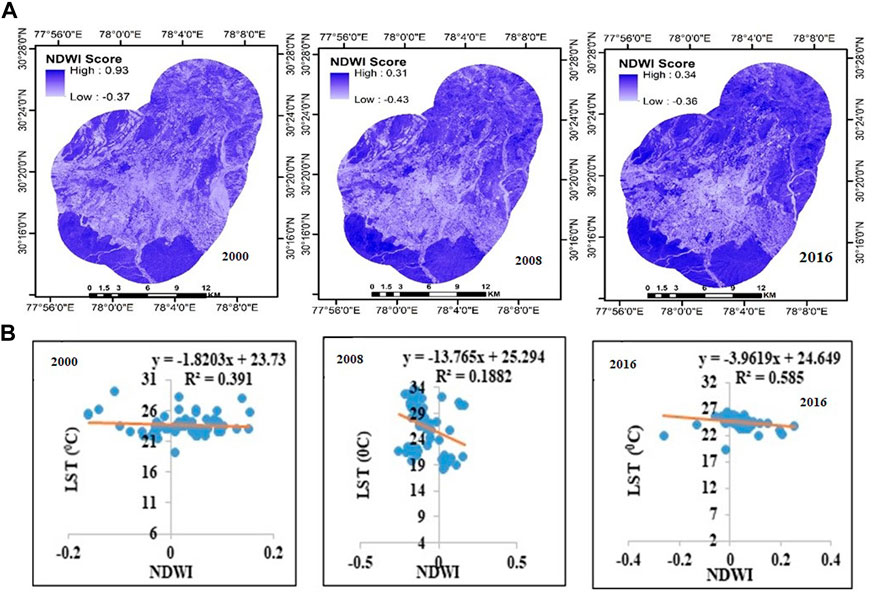
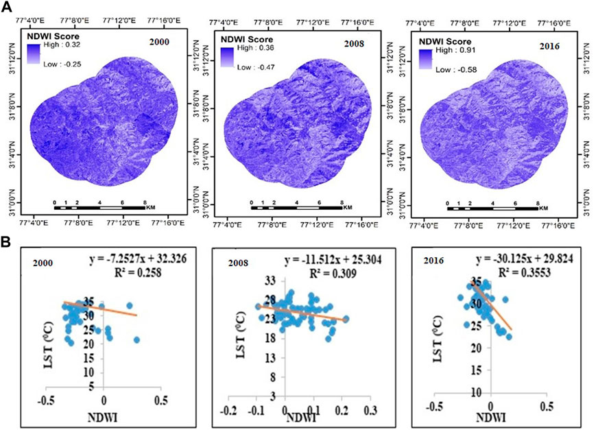
3.6 Association of NDWI with LST
The spatial pattern and distribution of NDWI for Dehradun and Shimla are shown in Figures 8A, 9A, respectively. NDWI provides the moisture content in areas where the temperature is typically lower than in other land uses (Zhang & Huang, 2015). The LST of water body in general lower than other kind of land use categories (Rao and Pant, 2001; Zhang & Huang, 2015). The level of NDWI control over LST for both cities throughout all time periods is shown in Figures 8B, 9B. It was discovered that NDWI adversely controls LST in every instance. For Dehradun, the R2 value increased from R2 = 0.05 in 2000 to R2 = 0.08 in 2008 and then to R2 = 0.58 in 2016. Like this, Shimla’s R2 value exhibits rising patterns from 2000 (R2 = 0.02) to 2008 (R2 = 0.10) and further in 2016. (R2 = 0.35). In the city’s center, a lower NDWI value was discovered, demonstrating the masking impact of built-up characteristics. Higher NDWI was noticed outside the core zone in all the periods for both cities.
3.7 Spatial metrics
3.7.1 Landscape fragmentation analysis at class level
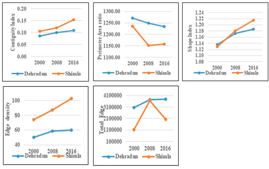
A solid conceptual and theoretical foundation for evaluating landscape structure, function, and change is quantified through the examination of class- and landscape-level measures. Landscape metrics allow to establish the relationship between the spatial properties of patches or landscapes and biological processes by focusing on changes in the area’s geometry, class size and land cover fragmentation (Nagendra et al., 2004). Area and edge metrics are concerned with the size of the patches and the amount of edge that each patch makes up. The lengths of all edge segments involving the relevant patch type are roughly added up to form Total Edge (TE). Figure 10 provides the class-level indicators for Dehradun and Shimla. To determine the shape complexity of the classified maps, the Shape Index was calculated. Greater shape complexity and hence greater changeability are indicated by a higher shape index. The patch is more susceptible to the edge effect as the shape index rises. Shimla’s ED, which measures the total edge of any class relative to the entire landscape (Seto and Fragkias, 2005), rises significantly from 2000 to 2016, while Dehradun’s rises strongly from 2000 to 2008 and then slowly from 2008 to 2016. This is caused by an increase in urban edge pixels, which shows the development of new urban edges and intricate structures. The total edge of any patch type at the class level or of all patch types at the landscape level is measured by TE (McGarigal and Mark, 1995). TE for Dehradun has increased during the study period showing the rapid expansion of the city with an increase in built-up structures while for Shimla it increases from 2000 to 2008 due to expansion of the city and then decreases which may be attributed to aggregation of built up structures as horizontal expansion can’t take place due to steep slopes of the hilly region. CONTIG measures the degree of spatial connectedness and urban dispersion. High CONTIG means low sprawling as it is related to the discontinuity of urban growth (Triantakonstantis and Stathakis, 2015). Over the course of the study period, CONTIG displays increased tendencies for both cities that show an increase in the connection of urban structures and a corresponding decline in sprawl. Although SI and PARA both measure shape complexity, SI is more representative of shape complexity because the former lacks uniformity. The SI for both cities has increased over the course of the study, which shows that urban areas are developing more intricate patterns. An increase in anthropogenic disturbances will result in increased fragmentation, which will indirectly result in a reduction in the area’s forest cover (Aditya et al., 2018).
3.7.2 Landscape fragmentation analysis at landscape level
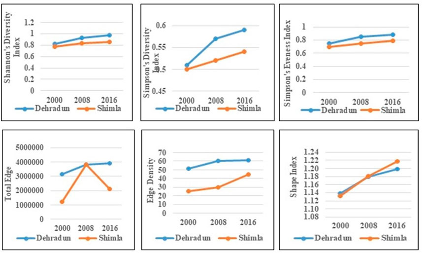
SHDI is a metric for gauging a community’s diversity. It rises as there are more and more varieties of patch. Figure 11 provides the landscape-level measures (SHDI, SIDI, and SIEI) for Dehradun and Shimla. For the years 2000–2016, the SHDI, SIDI, and SIEI showed rising trends for Dehradun and Shimla. The accelerated rate of urban sprawl may be to blame for this. This makes reference to the sprawling pattern as well. The build-up of Dehradun city has increased quickly and unevenly. This holds true over the course of the investigation. Although the development in built-up areas in Shimla is spatially scattered, it has also led to an increase in size and density. Shimla’s built-up area has been steadily expanding, followed by its size and population density.
4 Conclusion
Using change detection and landscape metrics, this study sought to understand and document how urbanization has affected the LST across Dehradun and Shimla. The two Himalayan cities of Uttarakhand and Himachal Pradesh in India are rapidly becoming urbanized. Land surface temperatures are rising as a result of the increased urbanization, which is causing land surfaces to be fragmented and covered in concrete and other impermeable materials. These cities are now experiencing higher temperatures than usual. The LST of the study area has increased as result of decline in land use classes such as forest, agriculture land and waterbodies and increase in concretization in the form of settlement. Increased urbanization impacts the general health of the landscape and makes it more vulnerable to fragmentation, which could significantly alter the area’s ecological functions and processes. We noticed urbanization and landscape fragmentation were occurring haphazardly. The outcome showed that the landscape in the research area was fragmented and heterogeneous from 2000 to 2008, after which it has aggregated and grown more heterogeneous. Except for aquatic bodies, lower LST were observed in areas with higher NDVI values, whereas greater LST were found in populated areas. Similar to other Indian cities, urban heat islands are emerging in the Himalayan cities too. According to this study, these changes were primarily attributable to shifts in natural variables like climate and anthropogenic changes such as population growth and its pressure, a rapidly expanding and structurally changing economy, a lack of land use planning, and ineffective implementation of existing policies. Decentralizing urban built-up areas and population distribution by radical urban infrastructure development policies toward the outskirts of the city can greatly mitigate the consequences of rising temperatures. The findings of this study demonstrate that, especially over the past few decades, human intervention in natural systems has multiplied. Even ecologically delicate ecosystems, like those in the Himalayas, are experiencing these massive human-environmental interactions, which have huge ramifications. In order to reduce population pressure and the strain on land resources, there is an urgent need to transition from horizontal to vertical housing construction. Laws that oppose the haphazard conversion of land resources particularly the conversion of forested land, should be introduced. The analysis of LST, land use and landscape fragmentation directed meticulous planning and policy implementation by concern authorities in order to preserve and maintain the rich ecological diversity of the two Himalayan cities.
Data availability statement
The raw data supporting the conclusions of this article will be made available by the authors, without undue reservation.
Author contributions
RG, MS and GS conceived the idea; RG, MS and GS, designed and analyzed the data; RG, MS, GS and RJ contributed materials/analysis tools; RG, wrote the manuscript and RJ, MS and GS edited the manuscript.
Funding
The author RG is thankful to the University Grant Commission, Govt. of India for providing the necessary financial support under Junior Research Fellowship scheme (NTA ref 190510396571).
Acknowledgments
The author acknowledges Spatial Analysis and Informatics Laboratory (SAIL), School of Environmental Science, Jawaharlal Nehru University, New Delhi, India, for providing the necessary facilities and expertise.
Conflict of interest
The authors declare that the research was conducted in the absence of any commercial or financial relationships that could be construed as a potential conflict of interest.
Publisher’s note
All claims expressed in this article are solely those of the authors and do not necessarily represent those of their affiliated organizations, or those of the publisher, the editors and the reviewers. Any product that may be evaluated in this article, or claim that may be made by its manufacturer, is not guaranteed or endorsed by the publisher.
References
Aditya, S. K., Smitha, A. V., Jenitha, J., and Rajesh, R. (2018). Landscape analysis using GIS and remote sensing for assessing spatial pattern in forest fragmentation in Shendurney Wildlife Sanctuary. India: Western Ghats, 299–304.2
Anees, M. M., Sajjad, S., and Joshi, P. K. (2018). Characterizing urban area dynamics in historic city of Kurukshetra, India, using remote sensing and spatial metric tools. Geocarto Int. 34, 1584–1607. doi:10.1080/10106049.2018.1499819
Artis, D. A., and Carnahan, W. H. (1982). Survey of emissivity variability in thermography of urban areas. Remote Sens. Environ. 12, 313–329. doi:10.1016/0034-4257(82)90043-8
Ashwini, K., and Sil, B. S. (2022). Impacts of land use and land cover changes on land surface temperature over cachar region, northeast India—a case study. Sustainability 14 (21)–14087. doi:10.3390/su142114087
Bhat, P. A., ul Shafiq, M., Mir, A. A., and Ahmed, P. (2017). Urban sprawl and its impact on landuse/land cover dynamics of Dehradun City, India. Int. J. Sustain. Built Environ. 6 (2), 513–521. doi:10.1016/j.ijsbe.2017.10.003
Bhatta, B. (2009). Analysis of urban growth pattern using remote sensing and GIS: A case study of Kolkata, India. Int. J. Remote Sens. 30 (18), 4733–4746. doi:10.1080/01431160802651967
Carlson, T. (2003). Applications of remote sensing to urban problems. Remote Sens. Environ. 86, 273–274. doi:10.1016/s0034-4257(03)00073-7
Chander, G., Markham, B. L., and Helder, D. L. (2009). Summary of current radiometric calibration coefficients for Landsat MSS, TM, ETM+, and EO-1 ALI sensors. Remote Sens. Environ. 113, 893–903. doi:10.1016/j.rse.2009.01.007
Chen, X. L., Zhao, H. M., Li, P. X., and Yin, Z. Y. (2006). Remote sensing image-based analysis of the relationship between urban heat island and land use/cover changes. Remote Sens. Environ. 104 (2), 133–146. doi:10.1016/j.rse.2005.11.016
Congalton, R. G., and Green, K. (1999). Assessing the accuracy of remotely sensed data: Principles and practices. Boca Raton: Lewis Publishers.
Dasgupta, A., Kumar, U., and Ramachandra, T. V. (2009). “Urban Landscape analysis through spatial metrics,” in Proceedings of International Conference on Infrastructure, Sustainable Transportation and Urban Planning, (CISTUP@ CiSTUP), Indian Institute of Science, Bangalore, India, 18–20.
Dewan, A. M., and Yamaguchi, Y. (2009). Using remote sensing and GIS to detect and monitor land use and land cover change in Dhaka Metropolitan of Bangladesh during 1960-2005. Environ. Monit. Assess. 150, 237–249. doi:10.1007/s10661-008-0226-5
Fenta, A. A., Yasuda, H., Haregeweyn, N., Belay, A. S., Hadush, Z., Gebremedhin, M. A., et al. (2017). The dynamics of urban expansion and land use/land cover changes using remote sensing and spatial metrics: The case of mekelle city of northern Ethiopia. Int. J. Remote Sens. 38, 4107–4129. doi:10.1080/01431161.2017.1317936
Gao, B. C. (1996). NDWI—A normalized difference water index for remote sensing of vegetation liquid water from space. Remote Sens. Environ. 58 (3), 257–266. doi:10.1016/s0034-4257(96)00067-3
Gautam, A. P., Webb, E. L., and Eiumnoh, A. (2002). GIS assessment of land use/land cover changes associated with community forestry implementation in the Middle Hills of Nepal. Mt. Res. Dev. 22 (1), 63–69. doi:10.1659/0276-4741(2002)022[0063:gaolul]2.0.co;2
Giridharan, R., Ganesan, S., and Lau, S. S. Y. (2004). Day time urban heat island effect in high-rise and high-density residential developments in Hong Kong. Energy Build. 36 (6), 525–534. doi:10.1016/j.enbuild.2003.12.016
Grover, A., and Singh, R. B. (2015). Analysis of urban heat island (UHI) in relation to normalized difference vegetation index (NDVI): A comparative study of Delhi and Mumbai. Environments 2015 (2), 125–138. doi:10.3390/environments2020125
Guha, S., Govil, H., Dey, A., and Gill, N. (2020). A case study on the relationship between land surface temperature and land surface indices in Raipur City, India. Bejing China: Geogr Tidsskr. doi:10.1080/00167223.2020.1752272
Harris, I., Osborn, T. J., Jones, P., and Lister, D. (2020). Version 4 of the CRU TS monthly high-resolution gridded multivariate climate dataset. Sci. Data 7, 109. doi:10.1038/s41597-020-0453-3
He, C., Shi, P., Xie, D., and Zhao, Y. (2010). Improving the normalized difference built-up index to map urban built-up areas using a semiautomatic segmentation approach. Remote Sens. Lett. 1 (4), 213–221. doi:10.1080/01431161.2010.481681
Herold, M., Couclelis, H., and Clarke, K. C. (2005). The role of spatial metrics in the analysis and modeling of urban land use change. Comput. Environ. Urban Sys 29, 369–399. doi:10.1016/j.compenvurbsys.2003.12.001
Herold, M., Liu, X., and Clarke, K. C. (2003). Spatial metrics and image texture for mapping urban land use. Photogram Eng. Remote Sens. 69, 991–1001. doi:10.14358/pers.69.9.991
Herold, M., Scepan, J., and Clarke, K. C. (2002). The use of remote sensing and landscape metrics to describe structures and changes in urban land uses. Environ. Plan. A 34, 1443–1458. doi:10.1068/a3496
Jalan, S., and Sharma, K. (2014). Spatio-temporal assessment of land use/land cover dynamics and urban heat island of Jaipur city using satellite data. Int. Arch. Photogramm. Remote Sens. Spat. Inf. Sci. XL- 8, 767–772. doi:10.5194/isprsarchives-xl-8-767-2014
Joshi, P. K., Lele, N., and Agarwal, S. P. (2006). Entropy as an indicator of fragmented landscape. Curr. Sci. 91, 276–278.
Joshi, P. K., Singh, S., Agarwal, S., and Roy, P. S. (2001). Forest cover assessment in Western Himalayas, Himachal Pradesh using IRS 1C/1D WiFS data. Curr. Sci. 80 (8), 941–947.
Keles, S., Sivrikaya, F., and Cakir, G. (2007). Temporal changes in forest landscape patterns in Artvin forest planning unit, Turkey. Environ. Monit. Assess. 129, 483–490. doi:10.1007/s10661-006-9380-9
Kuldeep, T., and Kamlesh, K. (2011). Land use/land cover change detection in Doon valley (Dehradun tehsil), uttrakhand: Using GIS and remote sensing technique. Int. J. Geomatics Geosciences 2 (1), 34–41.
Landsat Project Science Office, (2002).Landsat 7 science data user’s handbook Washington, DC. URL:Goddard Space Flight Center, NASA http://ltpwww.gsfc.nasa.gov/IAS/handbook/handbook_toc. html ((last date accessed: September 10, 2003).
Lilly Rose, A., and Devadas, M. D. (2009). Analysis of land surface temperature and land use/land cover types using remote sensing imagery - a case in Chennai city, India, the seventh international conference on urban clim. Yokohama, Japan. held on 29 June – 3 July 2009.
Liu, H., Zhan, Q., Yang, C., and Wang, J. (2018). Characterizing the spatio-temporal pattern of land surface temperature through time series clustering: Based on the latent pattern and morphology. Remote Sens. 10, 654. doi:10.3390/rs10040654
Mallick, J., Kant, Y., and Bharath, B. D. (2008). Estimation of land surface temperature over Delhi using Landsat-7 ETM+. J. Ind. Geophys. Union 12 (3), 131–140.
Mallick, J., Rahman, A., and Singh, C. K. (2013). Modeling urban heat islands in heterogeneous land surface and its correlation with impervious surface area by using night-time ASTER satellite data in highly urbanizing city, Delhi-India. Adv. Space Res. Space. Res. 5252 (4), 639639–655655. doi:10.1016/j.asr.2013.04.025
Martin, Balej (2012). Landscape metrics as indicators of the structural landscape changes – two case studies from the Czech Republic after 1948. J. Land Use Sci. 7 (4), 443–458. doi:10.1080/1747423X.2011.597443
McCarthy, M. P., Best, M. J., and Betts, R. A. (2010). Climate change in cities due to global warming and urban effects. Geophys. Res. Lett. 37–L09705. doi:10.1029/2010gl042845
McGarial, K. (2013). Fragstats, v.4 help. Available from: http://www.umass.edu/landeco/research/Fragstats/documents/fragstats.help.4.2.pdf.
McGarial, K., and Marks, B. (1995) Fragstat: Spatial pattern analysis program for quantifying landscape structure. Portland (OR): U.S. Department of Agriculture, Pacific Northwest Research Station. p. 12.
Midha, N., and Mathur, P. K. (2010). Assessment of forest fragmentation in the conservation priority Dudhwa landscape, India using FRAGSTATS computed class level metrics. J. Indian Soc. Remote Sens. 38 (3), 487–500. doi:10.1007/s12524-010-0034-6
Mishra, P. K., Rai, A., and Rai, S. C. (2020). Land use and land cover change detection using geospatial techniques in the Sikkim Himalaya, India. Egypt. J. Remote Sens. Space Sci. 23 (2), 133–143. doi:10.1016/j.ejrs.2019.02.001
Munsi, M., Malaviya, S., Oinam, G., and Joshi, P. K. (2009) A landscape approach for quantifying land-use and land-cover change (1976–2006) in middle Himalaya. Reg. Environ. Change, [Online] Volume 10(2), p. 145–155. doi:10.1007/s10113-009-0101-0
Munsi, M., Areendran, G., Ghosh, A., and Joshi, P. (2010). Landscape characterisation of the forests of Himalayan foothills. Journal of the Indian Society of Remote Sensing 38 (3), 441–452. doi:10.1007/s12524-010-0046-2
Nagendra, H., Munroe, D., and Southworth, K. (2004) From pattern to process: Landscape fragmentation and the analysis of land use/land cover change. Elsevier J. Agric. Ecosyst. Environ., [Online] Volume 101(2-3), p. 111–115. doi:10.1016/j.agee.2003.09.003
Neteler, M. (2010). Estimating daily land surface temperatures in mountainous environments by reconstructed MODIS LST data. Remote Sens. 2, 333–351. doi:10.3390/rs1020333
Ogashawara, I., and Bastos, V. D. S. B. (2012). A quantitative approach for analyzing the relationship between urban heat islands and land cover. Remote Sens. 4 (11), 3596–3618. doi:10.3390/rs4113596
Pal, S., and Ziaul, S. K. (2017). Detection of land use and land cover change and land surface temperature in English Bazar urban Centre. Egypt. J. Remote Sens. Space Sci. 20 (1), 125–145. doi:10.1016/j.ejrs.2016.11.003
Peng, J., Ma, J., Liu, Q., Liu, Y., Hu, Y., Li, Y., et al. (2018). Spatial-temporal change of land surface temperature across 285 cities in China: An urban-rural contrast perspective. Sci. Total Environ. 635, 487–497. doi:10.1016/j.scitotenv.2018.04.105
Prastakos, P., Chrysoulakis, N., and Kochilakis, G. (2012). “Spatial metrics for Greek cities using land cover information from the Urban Atlas,” in Proceedings of the AGILE’2012 international conference on geographical information science; april 24–27; multidisciplinary research on geographical information in europe and beyond. Editors J. Gensel, D. Josselin, and D. Vandenbroucke (Avignon, 261–266.
Punia, M., and Singh, L. (2012). Entropy approach for assessment of urban growth: A case study of Jaipur, India. J. Indian Soc. Remote Sens. 40 (2), 231–244. doi:10.1007/s12524-011-0141-z
Ramachandra, T. V., Bharath, H., and Durgappa, D. (2012b). Insights to urban dynamics through landscape spatial pattern analysis. Int. J. Appl. Earth Obs. Geoinf 18, 329–343. doi:10.1016/j.jag.2012.03.005
Rao, K. S., and Pant, R. (2001). Land use dynamics and landscape change pattern in a typical micro watershed in the mid elevation zone of central Himalaya, India. Agric. Ecosyst. Environ. 86 (2), 113–124. 10.1016/s0167-8809 (00)00274-7.
Rashid, N., Alam, J. M., Chowdhury, M. A., and Islam, S. L. U. (2022). Impact of landuse change and urbanization on urban heat island effect in narayanganj city, Bangladesh: A remote sensing-based estimation. Environ. Challenges 8–100571. doi:10.1016/j.envc.2022.100571
Rawat, J. S., and Kumar, M. (2015). Monitoring land use/cover change using remote sensing and GIS techniques: A case study of hawalbagh block, district almora, Uttarakhand, India. Egypt. J. Remote Sens. Space Sci. 18, 77–84. doi:10.1016/j.ejrs.2015.02.002
Roy, P. S., and Tomar, S. (2001). Landscape cover dynamics pattern in Meghalaya. Int. J. Remote Sens. 22 (18), 3813–3825. doi:10.1080/01431160010014008
Seto, K. C., and Fragkias, M. (2005). Quantifying spatiotemporal patterns of urban land-use change in four cities of China with time series landscape metrics. Landsc. Ecol. 20, 871–888. doi:10.1007/s10980-005-5238-8
Sharma, R., and Joshi, P. K. (2012). Monitoring urban landscape dynamics over Delhi (India) using remote sensing (1998-2011) inputs. J. Indian Soc. Remote Sens. 41 (3), 641–650. doi:10.1007/s12524-012-0248-x
Sobrino, J. A., Jime´nez-Muoz, J. C., and Paolini, L. (2004). Land surface temperature retrieval from Landsat TM5. Remote Sens. Environ. 90 (4), 434–440. doi:10.1016/j.rse.2004.02.003
Srinivasan, K., Sebastian, A., Menachery, M. P., and Pant, G. (2022). Landscape fragmentation analysis in and around Rajaji national park, Uttarakhand, India. Indian J. Ecol. 49 (2), 590–595.
Story, M., and Congalton, R. G. (1986). Accuracy assessment: A user’s perspective. Photogramm. Eng. Remote Sens. 52, 397–399.
Tou, J. T., and Gonzalez, R. C. (1974). Analysis of urban growth pattern using remote sensing and GIS: A case study of Kolkata, India. Int. J. Remote Sens. 30 (18), 4733–4746. doi:10.1080/01431160802651967
Wakode, H. B., Baier, K., Jha, R., and Azzam, R. (2014). Analysis of urban growth using Landsat TM/ETM data and GIS-a case study of Hyderabad, India. Arab. J. Geosci. 7, 109–121. doi:10.1007/s12517-013-0843-3
Weng, Q., and Lu, D. (2008). A sub-pixel analysis of urbanization effect on land surface temperature and its interplay with impervious surface and vegetation coverage in Indianapolis, United States. Int. J. Appl. Earth Observation Geo-information 10, 68–83. doi:10.1016/j.jag.2007.05.002
Weng, Q., Lu, D., and Schubring, J. (2004). Estimation of land surface temperature– vegetation abundance relationship for urban heat island studies. Remote Sens. Environ. 89 (4), 467–483. doi:10.1016/j.rse.2003.11.005
Weng, Q., and Yang, S. (2004). Managing the adverse thermal effects of urban development in a densely populated Chinese city. J. Environ. Manag. 70, 145–156. doi:10.1016/j.jenvman.2003.11.006
Xiao, H., and Weng, Q. (2007). The impact of land use and land cover changes on land surface temperature in a karst area of China. J. Environ. Manag. 85, 245–257. doi:10.1016/j.jenvman.2006.07.016
Yu, X., and Ng, C. (2006). An integrated evaluation of landscape change using remote sensing and landscape metrics: A case study of panyu, guangzhou. Int. J. Remote Sens. 27 (6), 1075–1092. doi:10.1080/01431160500377162
Zha, Y., Gao, J., and Ni, S. (2003). Use of normalized difference built-up index in automatically mapping urban areas from TM imagery. Int. J. Remote Sens. 24 (3), 583–594. doi:10.1080/01431160304987
Zhang, W., and Huang, B. (2015). Land use optimization for a rapidly urbanizing city with regard to local climate change: Shenzhen as a case study. J. Urban Plan. Dev. 141 (1)–05014007. doi:10.1061/(asce)up.1943-5444.0000200
Keywords: urban sprawl, normalized difference vegetation index (NDVI), normalized difference water index (NDWI), normalized difference built-up index (NDBI), land surface temperature (LST), spatial metrics
Citation: Gupta R, Sharma M, Singh G and Joshi RK (2023) Characterizing urban growth and land surface temperature in the western himalayan cities of India using remote sensing and spatial metrics. Front. Environ. Sci. 11:1122935. doi: 10.3389/fenvs.2023.1122935
Received: 13 December 2022; Accepted: 11 January 2023;
Published: 19 January 2023.
Edited by:
Cletah Shoko, University of the Witwatersrand, South AfricaReviewed by:
Polina Lemenkova, Université libre de Bruxelles, BelgiumGui Jin, China University of Geosciences Wuhan, China
Copyright © 2023 Gupta, Sharma, Singh and Joshi. This is an open-access article distributed under the terms of the Creative Commons Attribution License (CC BY). The use, distribution or reproduction in other forums is permitted, provided the original author(s) and the copyright owner(s) are credited and that the original publication in this journal is cited, in accordance with accepted academic practice. No use, distribution or reproduction is permitted which does not comply with these terms.
*Correspondence: Rajendra Kr Joshi, cmFqZW5kcmFrcmpvQGdtYWlsLmNvbQ==; Rajman Gupta, cmFqbWFuZ3VwdGE2MUBnbWFpbC5jb20=
 Rajman Gupta
 Mani Sharma
 Garima Singh
 Rajendra Kr Joshi