 Maximilian Barczok
 Chelsea Smith2
 Nicolle Di Domenico
 Elizabeth Herndon
95% of researchers rate our articles as excellent or good
Learn more about the work of our research integrity team to safeguard the quality of each article we publish.
Find out more
ORIGINAL RESEARCH article
Front. Environ. Sci. , 07 July 2023
Sec. Biogeochemical Dynamics
Volume 11 - 2023 | https://doi.org/10.3389/fenvs.2023.1114814
This article is part of the Research Topic Hydrology, Ecology, and Nutrient Biogeochemistry at the Terrestrial-Aquatic Interface View all 8 articles
Vernal ponds are ephemeral landscape features that experience intermittent flooding and drying, leading to variable saturation in underlying soils. Redox potential (Eh) is an important indicator of biogeochemical processes that changes in response to these hydrological shifts; however, high-resolution measurements of Eh in variably inundated environments remain sparse. In this study, the responses of soil Eh to ponding, drying, and rewetting of a vernal pond were investigated over a 5-month period from late spring through early autumn. Soil Eh was measured at 10-min frequencies and at multiple soil depths (2–48 cm below the soil surface) in shallow and deep sections within the seasonally ponded lowland and in unsaturated soils of the surrounding upland. Over the study period, average Eh in surface soils (0–8 cm) was oxidizing in the upland (753 ± 79 mV) but relatively reducing in the shallow lowland (369 ± 49 mV) and deep lowland (198 ± 37 mV). Reducing conditions (Eh <300 mV) in surface soils prevailed for up to 6 days in the shallow lowland and up to 24 days in the deep lowland after surface water dried out. Intermittent reflooding resulted in multiple shifts between reducing and oxidizing conditions in the shallow lowland while the deep lowland remained reducing following reflooding. Soil Eh in the uplands was consistently oxidizing over the study period with transient increases in response to rain events. Reducing conditions in the lowland resulted in greater Fe-oxide dissolution and release of dissolved Fe and P into porewater than in the surrounding uplands. We determined that change in water depth alone was not a good indicator of soil Eh, and additional factors such as soil saturation and clay composition should be considered when predicting how Eh responds to surface flooding and drying. These findings highlight the spatial and temporal variability of Eh within ponds and have implications for how soil processes and ecosystem function are impacted by shifts in hydrology at terrestrial-aquatic interfaces.
Redox potential in soils is an important factor in determining biogeochemical cycling of elements (Kappler et al., 2021; Zhang and Furman, 2021), mobility of trace elements (Mansfeldt and Overesch, 2013), cycling of nutrients (Peretyazhko and Sposito, 2005), emission of greenhouse gases (Yu and Patrick, 2004), and formation of redoximorphic features (Reddy and DeLaune, 2008). Redox potential is represented by the standard reduction potential (Eh), which is defined as the potential of a chemical species to accept electrons and be reduced, e.g., Fe3+ + e− → Fe2+, and is reported as a voltage measurement relative to the standard hydrogen electrode (SHE). Oxidized species (e.g., O2, NO3−, FeIII, SO42− CO2) are abundant at high Eh (> 400 mV), indicating a propensity to accept electrons, while reduced species that serve as electron donors (e.g., NH4+, FeII, H2S, CH4) become more abundant with decreasing Eh. In the soil, Eh measurements are influenced by many factors such as oxygen availability (Glinski and Stepniewski, 1985; Mansfeldt, 2003), pH (Fiedler et al., 2007), temperature (Dorau et al., 2021), and biological activity (Kappler et al., 2021) and can vary widely over short distances (Fiedler et al., 2007; Reddy and Delaune, 2008).
Redox potential in soils and sediments is largely driven by O2 availability, which is controlled by diffusion from the atmosphere into the soil profile and by consumption through microbial and root respiration. Oxygen diffuses much more slowly in water than in air; thus, oxygen typically becomes depleted with increasing depth below the soil surface (Rubol et al., 2012; Peralta et al., 2014), leading to a more reducing environment deeper in the soil profile (Zhang and Furman, 2021). Oxidation of organic matter (OM) is a primary driver of O2 consumption as microorganisms use OM as a terminal electron acceptor. An abundance of OM therefore can increase the O2 consumption of a system by increased aerobic respiration (LaRowe and Van Cappellen, 2011). The classic representation of a redox ladder can be constructed with common redox pairs, where a sequence of oxidized species starting with O2 are progressively consumed to produce reduced species as redox potential decreases, generating conceptual biogeochemical depth profiles within soils or sediments (Zhang and Furman, 2021). However, soils are heterogeneous environments that experience high spatial and temporal variability in saturation. For example, the capillary fringe is a transition zone between saturated and unsaturated zones of soil where water migrates from the saturated zone to partially fill pores (Zhang and Furman, 2021). Soils in the capillary fringe experience sharp saturation differences over short distances and with time (Rühle et al., 2015) and can act as hot spots for biogeochemical activity (Ronen et al., 2000; McClain et al., 2003; Rezanezhad et al., 2014). Additionally, lateral flow can introduce oxygenated water and raise soil Eh at depth (D’Amore et al., 2004), contrary to expectations discussed above. Furthermore, how redox potential reacts to hydrologic disturbance depends on the redox buffering capacity of the system, i.e., the ability of the system to resist change due to the abundance of particular chemical species that must be consumed before redox can shift (Burgin and Loecke, 2023). Predictions of soil Eh and biogeochemical processes therefore depend on multiple factors that are not totally understood.
An increasingly common method to measure redox potential in soils is by the use of Pt electrodes in combination with Ag0/AgCl reference probe with an internal saturated electrolyte solution (Mansfeldt, 2003; Dorau et al., 2018a; Zhang and Furman, 2021). These probes are then connected to a voltmeter to measure the electron transfer between the reference solution and the Pt electrodes. Positive recorded voltage (high E) represents flow of electrons from the reference probe to the Pt electrode and negative voltage (low E) represents flow from the Pt electrode to the reference probe. Recorded redox potentials are adjusted relative to the SHE to produce Eh values that are comparable across studies. While many redox reactions can happen simultaneously and contribute to a mixed signal (Rivett et al., 2008), this measurement is dominated by the redox couples with the highest exchange currents (Mansfeldt, 2003; Markelova, 2017; Dorau et al., 2018b). For example, many studies have shown that Pt electrodes respond strongly to changes in the electroactive Fe2+-Fe3+ redox pair and are therefore useful to detect the occurrence of dissolved and absorbed Fe2+ (Cogger et al., 1992; Mansfeldt, 2004; Dorau et al., 2018b). Broadly, Mansfeldt (2003) assigned Eh classifications of oxidizing (> 400 mV), weakly reducing (400–200 mV), moderately reducing (200 to −100 mV) and strongly reducing (<−100 mV) conditions to soils at pH 7. A threshold between reducing and oxidizing conditions has been proposed at 300 mV by Reddy and DeLaune (2008) and is often used to distinguish between aerobic and anaerobic conditions (Dorau et al., 2018a; Zhang and Furman, 2021).
Previous studies investigating soil redox conditions have focused on relationships between Eh and soil morphology (Fiedler and Sommer, 2004; Dorau et al., 2018a), distribution of elements in soils (Fiedler and Sommer, 2004; Mansfeldt, 2004), and production of methane (Yu et al., 2007; Fiedler and Sommer, 2004; Street et al., 2016), as well as the use of Pt electrodes to monitor soil Eh for the purpose of improving agricultural management practices (Husson et al., 2016). Much of the existing research on soil redox potential focuses on comparing one stable environment to another stable environment with less emphasis on changes over time in response to dynamic hydrology (Zhang and Furman, 2021). For example, wetland systems are often studied during periods of a high or low water table (Mansfeldt, 2003; Thomas et al., 2009) or perched water tables during dry or wet years (Dorau et al., 2021). However, recent developments in in situ redox sensors enable more detailed investigation into how soil redox fluctuates in response to changes in the water table. For example, redox response to tidal fluctuation and storm events exhibits lag times that depend at least in part on sediment properties (Wallace et al., 2019; Wallace and Soltanian, 2021; Yu et al., 2023). Additional work in permafrost landscapes shows that reducing conditions can develop seasonally in shallow soils but be disrupted by large rain events that introduce oxygenated water (Street et al., 2016). However, continuous measurements of Eh and associated hydrologic and biogeochemical parameters are still sparse, limiting our understanding of the timescales over which hydrologic disturbance affects redox potential, microbial activity, and solute mobility. More studies are therefore needed to evaluate how redox potential and associated biogeochemical processes vary in space and time across diverse environments.
In this study, we investigate how soil Eh responds to seasonal hydrologic change in and around a vernal pond. Vernal ponds are small, ephemeral wetlands that are often located in forests and can persist for three to 11 months in temperate and boreal climates of Europe and North America (Colburn, 2004). They generally flood in spring and fall during wetting conditions caused by higher precipitation, remain flooded or freeze during winter, and dry out in summer due to low precipitation and/or high evapotranspiration. Water sources for vernal ponds can include snowmelt, groundwater, surface runoff, and are often dominated by direct precipitation (Smith and Verrill, 1998; Bauder, 2005). Thus, vernal ponds provide wet-and-dry cycles that provide contrasting and fluctuating hydrological conditions. The objective of this study is to assess how soil Eh and associated biogeochemical indicators change with depth in and around a vernal pond in response to drying and rewetting. We hypothesize that the upland around the vernal pond will remain relatively static in Eh during the season while the flooded lowland will experience a fast shift from reducing to oxidation conditions or vice versa as hydrological conditions change from flooded to dry or dry to flooded. We also hypothesize that Eh decreases with depth and that deeper soils experience less Eh fluctuation over the season than shallow soils. Additionally we hypothesize that flooded conditions result in higher concentrations of dissolved iron (Fe) and phosphate in sediment pore water and surface waters.
This study was conducted in a vernal pond in Jennings Woods, a 0.3-km2 hardwood temperate forest owned by Kent State University near Ravenna, Ohio, United States (41.177004°N, −81.205108°W) that has been unmanaged since 1973. Average summer (June to August) temperature and precipitation at this site are 17.54°C and 422 mm, respectively (National Oceanic Atmospheric Agency/National Centers for Environmental Information, 2021). Precipitation data reported here were retrieved from a rain gauge approximately 8 km southwest of the study area (USC00336949). Dominant soils are in the Chili loam series (fine-loamy, mesic Typic Hapludalf) and Geeburg-Glenford silt loam complexes (both Aquic Hapludalfs, but Geeburg is illitic and Glenford has a mixed clay mineralogy) (Blackwood et al., 2013). The vernal pond studied is located at an upland plateau approximately 15–20 m elevated relative to the regional water table, as indicated by a nearby stream. The plateau includes several vernal ponds that flood primarily in response to precipitation in early spring and dry out over the summer months before reflooding in fall due to increased precipitation and decreased evapotranspiration (Blackwood et al., 2013). The approximate length of the study pond was 20 m with a width of 10 m (Figure 1). Polyvinyl chloride pipes were placed at random in the upland (n = 10) and lowland soils (n = 10) and used as location markers for site characterization (Figure 1). Differences in elevation relative to the upland redox probe were determined by measuring the difference in height of upland site 9 to each site in the lowland with a laser on 19th July 2018 when the pond had no surface water. The west portion of the pond (−48 ± 2 cm relative to site 9) was found to be consistently deeper than the east portion (−42 ± 3 cm relative to site 9) (Table 1; Supplementary Table S1). The west portion of the pond is therefore referred to as the deep lowland and the east portion of the pond is referred to as the shallow lowland from here on.
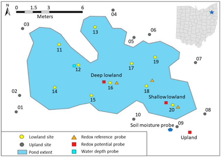
FIGURE 1. Extent of the vernal pond (delineated 10th May 2018) and location of the upland sites (numbered 01–10) and the lowland sites (numbered 11–20), redox reference probes, redox potential probes, soil moisture probes, and water depth probe. Map projection GCS WGS 1984 UTM 17N created with ArcGIS Pro 2020.
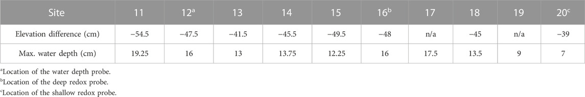
TABLE 1. Elevation difference of each lowland position relative to the upland site and maximum water depth measured manually at each site during the study period.
A water level logger (HOBO, U20L) was deployed in the deeper part of the pond near site 12 (47.5 cm below the upland site) and continuously (every 15 min) recorded air pressure plus water pressure. Water depth was calculated by correcting for air pressure with a second probe that was attached to a nearby tree according to manufacturer instructions (Onset Computer Corporation, 2020). Data were also corrected for slight depth offsets created by logger movement during removal for data downloads. Water depth at the location of the redox probe in the shallow lowland (site 20) was estimated by subtracting 8 cm, the elevation difference between site 12 and site 20, from the water depth measured at site 12. Two soil moisture sensors (ECH2O EC-5, METER) were deployed within 1.5 m of each other in the upland soil (Figure 1). The sensors were installed at a 45-degree angle to prevent preferential flow in the surface soil and recorded soil moisture over the top 5 cm soil depth every 15 min.
Soil redox potential was continuously (every 30 s) monitored with three redox potential probes (PaleoTerra) deployed in either the upland (n = 1) or the lowland (n = 2) soils from 15th June 2018 to 18th October 2018. In the lowland, one probe was placed in the shallow pond near site 20 where the soil surface was 39 cm below the soil surface of the upland site. The other probe was placed in the deeper part of the pond near site 16 where the soil surface was 48 cm below the upland site (Figure 1; Table 1). Each redox probe had eight 8 mm Pt sensors positioned at 2 cm, 4 cm, 6 cm, 8 cm, 10 cm, 20 cm, 30 cm, and 48 cm below the soil surface. Each Pt electrode is sensitive to its immediate surroundings and is not suitable to represent microsite variability or the redox potential of the entire pond (Fiedler et al., 2007). Redox potential was referenced to a Ag0/AgCl reference electrode deployed within the pond near the redox probes. Two additional reference electrodes were deployed in the pond as quality controls on the primary reference probe. Data were recorded at 30 s increments (CR1000 datalogger, Campbell Scientific) and averaged over 10-min increments. Retrieved data were adjusted to the standard hydrogen electrode (SHE) by adding 213 mV to the recorded values as recommended by PaleoTerra. Redox potential was not adjusted for pH but was interpreted in context of Eh ranges under acidic conditions. Variations in Eh due to temperature are expected to be ∼1 mV/°C and thus small between sites and depth (< 50 mV). Measurements above 300 mV are considered oxidizing and values below are considered reducing for the purpose of this study (Thamdrup, 2000). This boundary roughly corresponds to the redox potential of various Fe (III)-oxide minerals at moderately acidic pH (Kappler et al., 2021), and we evaluate Fe redox cycling using biogeochemical indicators discussed below. Redox potential probes were deployed 14th June 2018 but the first day of data was discarded as recommended by Fiedler et al. (2007) to allow the redox potential of the soil to equilibrate after disturbing it by inserting the probes.
Eight indicators of reduction in soils (IRIS) probes were deployed on July 5th to evaluate redox conditions represented by dissolution of Fe oxides. These probes were PVC pipes (50 cm long, 21 mm outside diameter) coated with a ferrihydrite/goethite mixture (Rabenhorst and Burch, 2006). Inserting the probes into the soil exposes the ferrihydrite/goethite mixture to the local redox potential and allow for reduction of Fe (III). Reduced Fe (III) will dissolve and reveal the white PVC under the reddish Fe oxide paint allowing to quantify how much Fe oxide was lost and estimate the redox potential based on that loss. A picture of each side of each probe was taken before deployment using a standardized camera and lighting setup. A 25 mm diameter soil auger was used to dig a hole into the soil before deploying the IRIS probe in order to avoid loss of the coating by pushing the probe into the ground. The lowland probes (n = 4) were place next to markers 12, 16, 17, and 20. The upland probes (n = 4) were placed next to markers 1, 5, 8, and 9 (Figure 1). IRIS probes deployed in the lowland and upland were removed after 2 weeks.
Pictures of each side of each probe were taken after removal using the same setup and lighting as for the initial photos. Iron oxide coating loss was quantified by comparing the loss of red color from the pre-deployment picture with the post-deployment picture using paint.net (version 4.1.1). The following analysis was repeated for all probes. First, the background was removed by using the wand function with a contiguous setting and a 20% tolerance. Any pixels left that were not connected to the tube were removed manually. The wand function was then used in the global flood mode with a tolerance of 80% on a white dot created outside the tube and all selected pixels were painted white. These pixels represent areas in which iron oxide paint was lost. The white dot was used to ensure comparable results along all pictures, and a tolerance setting of 80% was visually determined to best represent Fe oxide loss. The remaining pixels were colored black to represent areas with Fe oxide paint. Pixels were then counted and a percentage of are coated by Fe oxide paint was calculated. The difference of that percentage between pre- and post-deployment was used to calculate Fe oxide loss.
Nine micro soil moisture samplers (0.15 µm pore size, Simpler) were deployed at 5 cm depth in the upland soils (n = 6; markers 1, 2, 3, 5, 6, and 9) and lowland pond sediments (n = 3; Pipe 13, 15, and 20) to collect pore water. Syringes were used to generate vacuum on the macrorhizons and pull pore water into each syringe over a period of 7 days for each week that water was present. Water samples from the first 7 days of collection were discarded to account for disturbance. Pore waters from different samplers were combined into either upland or lowland samples on each date to generate sufficient volume for analyses. Additionally, surface water (when present) was collected from an undisturbed location in the pond by filling a 100 mL plastic bottle. Each water sample was filtered through a 0.45 μm cellulose acetate syringe filter (Sterilitech). Filtered water was partitioned into subsamples and acidified with two drops of concentrated ultrapure nitric acid (67%–70% by w/w, VWR Analytics) in the field for inductively coupled plasma optical emission spectroscopy (ICP-OES) (total Fe, P, Ca, Mg, Al, and Mn), acidified with concentrated ultrapure hydrochloric acid for analysis of dissolved organic C (Shimadzu TOC-L), or left unacidified and refrigerated for soluble reactive phosphorus (SRP) quantification within 2 weeks by the molybdate blue method (Murphy and Riley, 1962) using an automated flow analyzer (Lachat). Field method blanks and duplicates were also analyzed (Supplementary Table S2).
Two soil cores were collected from the lowland near sites 16 and 20 on 18th October 2018 using a 10 cm diameter soil auger. Soil was removed in approximately 5 cm increments from 0 to 20 cm depth and then in 10 cm increments from 20 to 60 cm depth. No soil core could be collected from the upland site due to a dense root network. Soils were air-dried and then oven dried at 40°C to constant mass. Soil pH was measured by mixing 1 g of dried subsample with 10 mL of ultrapure water (Milli-Q, 18 MΩ) and measuring the pH of the solution after 10 min. To determine soil particle and aggregate size, bulk dried soil was sieved to 1 mm, and the >1 mm fraction was weighed. The size distributions of soil aggregates and particles <1 mm were then analyzed with a Malvern™ Mastersizer 2,000 laser diffraction particle size analyzer equipped with a Hydro 2,000 MU manual inlet system. Size fractions are reported as the proportion of clay and silt size particles (<0.053 mm), fine sand and microaggregates (0.053–0.25 mm), medium to coarse sand and small macroaggregates (0.25–1 mm), and large macroaggregates and particles (>1 mm). Subsamples of dried soil were ground into a fine powder using tungsten carbide grinding balls in a ball mill for 5 min (8,000 M SPEX). Carbon and nitrogen concentrations were measured on triplicate subsamples of milled powder (∼5–7 mg) via combustion with an elemental analyzer (Costech ECS 4010). Milled subsamples were used for X-ray Diffraction (XRD) analysis to identify crystalline minerals. Samples were analyzed as a loose powder at 15 Amps and 40 kV at a theta 2 angle of 3°–90°. Fitting of the XRD spectra was done against the Crystallographic Open Database as a reference library. Relative abundance of minerals was determined by the Whole Pattern Powder Fitting method and a Reitveld Refinement with Rigaku’s PDXL software.
Error is reported either as analytical error for the instrument or as the standard error of the mean for averages across multiple measurements unless otherwise stated. Significant differences in Eh averaged over time for each location were determined with a one-way ANOVA as well as for both shallow subsurface (≤8 cm) and deeper subsurface (>8 cm) at each location (α = 0.05) in SigmaPlot 13.0. The separation of the shallow and deeper subsurface at 8 cm was selected to separate trends observed in the redox data. To assess differences in how much Eh varied over the study period at different sites, we calculated the average of the standard deviation in Eh for each depth at each location. Spearman correlation coefficients were calculated to determine the non-linear relationships between soil Eh and solutes measured in surface water and porewater. Porewater from upland soils was compared to upland soil Eh averaged over the top 8 cm on each date that porewater was collected. Surface water and porewater from the lowland soils were compared to soil Eh averaged over the top 8 cm of both the shallow and deep lowland sites on each date that porewater was collected.
Precipitation during the study period (June 15th to November 28th) totaled 642 mm with a maximum daily precipitation of 68 mm. The largest daily event occurred September 10th (68 mm) with a total precipitation of 103 mm over a 5-day period (September 7th to 11th). Air temperature averaged 19.6°C ± 5.0°C from June 15th to October 18th with a maximum recorded temperature of 31.3°C, a minimum of 1°C, and ≤3°C–15°C diurnal fluctuations. Temperatures were consistently high (20.2°C ± 3.9°C) through early September before decreasing through mid-October (7.8°C ± 3.2°C) (Figure 2).
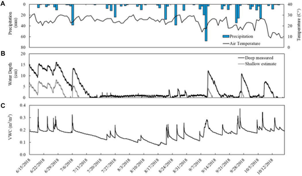
FIGURE 2. Environmental data collected from a temperate vernal pond (Ravenna, OH) from June 15th to October 18th. (A) Daily precipitation (collected approximately 8 km SW) and daily maximum temperature. (B) Water depth measured in the deep site of the pond (black) and the estimated water depth in the shallow site (grey). Water depth probe output fluctuated between 0–1 cm depth when no surface water was present. (C) Soil moisture in upland soils, recorded as volumetric water content.
Soil moisture in the upland averaged 0.196 ± 0.021 m3 m−3 from June 15th to July 8th before declining to a minimum of 0.072 m3 m−3 in August. Soil moisture then steadily rose again to an average 0.204 ± 0.024 m3 m−3 from September to October. Sharp increases in soil moisture coincided with precipitation events and were followed by slower declines (Figure 2).
Surface water depth measured manually decreased over time and was negligible on the shallow side of the vernal pond by June 28th and across the entire pond by July 5th (Supplementary Table S1). Water depth measured continuously at the deepest point of the vernal pond with the automated probe was initially 12 cm and increased to 16 cm by the end of June before decreasing to zero from July through mid-October (Figure 2). This location in the pond intermittently flooded three times in response to major rain events between August and October, reaching a maximum water depth of 12 cm. Water depth fluctuated between 0 and 1 cm and also recorded negative depths when there was no surface water, and surface water is therefore be assumed to be negligible during these measurements. Water depth in the shallow portion of the pond was estimated to experience a longer dry period from early July to September with less accumulation of surface water in response to precipitation events. In September, three rain events (September 9th; September 26th; October 7th) caused transient flooding for about 1 week each followed by short dry periods.
Carbon and nitrogen were high in the top 5 cm of both the shallow lowland (C = 15.5 ± 0.2%, N = 1.2 ± 0.0%) and deep lowland (C = 13.5 ± 0.4%, N = 1.1 ± 0.0%) and decreased with depth to below detection limit by 10–15 cm (<0.22 mg°C; <0.02 mg°N) (Table 2). Soils were dominated by quartz, clays (vermiculite and kaolinite), K-feldspar, plagioclase feldspar, and mica (Table 3). The soil core from the deep lowland had a higher quartz fraction (72.4% ± 2.1% vs. 59.8% ± 3.5%, respectively) and lower clay fraction (vermiculite vs. kaolinite; 8.1% ± 1.5% and 14.8% ± 2.8%, respectively) than the core from the shallow lowland. Quartz fractions were highest at 50–60 cm both in the shallow and deep lowland core (73% and 83%, respectively), while clay fractions were highest in the 5–10 cm depth (24% and 16%, respectively). Soil cores in both the shallow and deep lowland were dominated by clay and silt (47.9% ± 4.7% and 46.3% ± 4.4%, respectively) and large macroaggregates (37.4% ± 1.9% and 33.3% ± 3.5%, respectively). Smaller contributions in both the shallow and deep lowland come from microaggregates (7.2% ± 1.0% and 10.3% ± 1.2%) and small macroaggregates (7.4% ± 2.2% and 10.0% ± 1.8%) (Table 3). Clay and silt contents increased while small and large macroaggregates decrease with depth and were largely similar between cores.
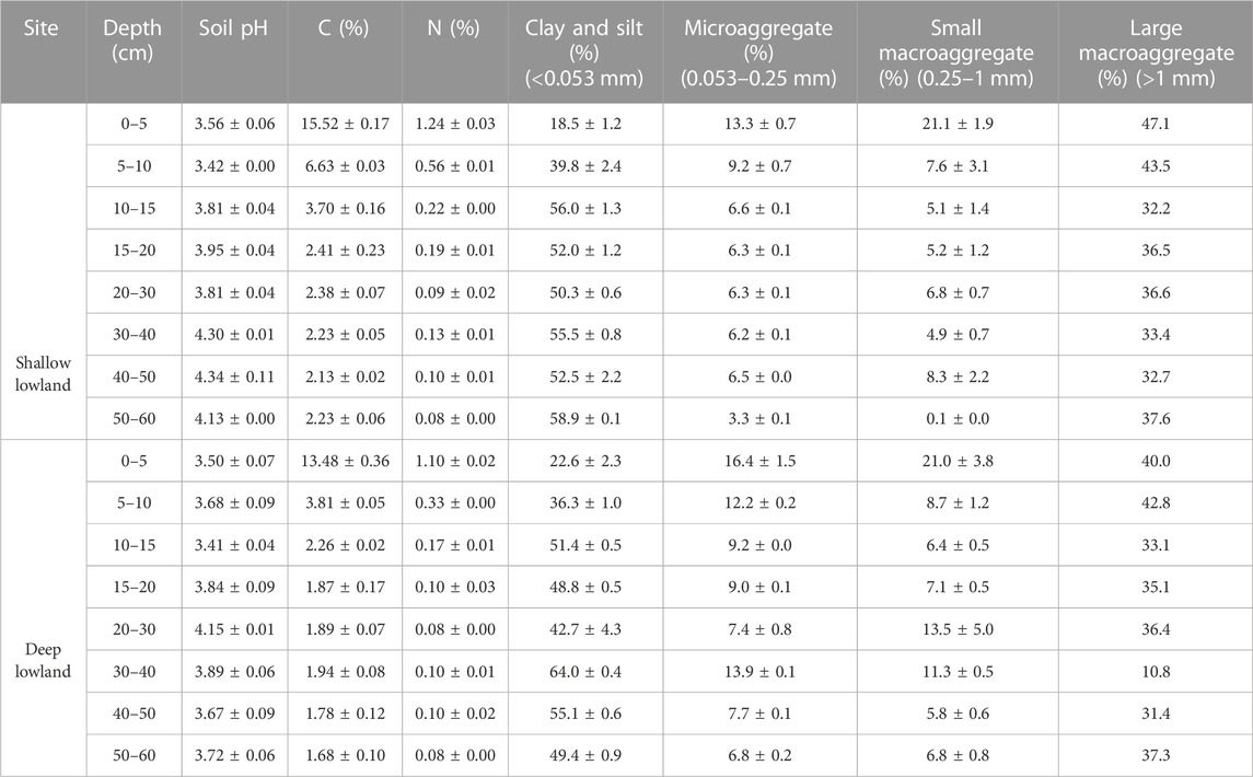
TABLE 2. Summary of soil properties of the shallow and deep lowland core.
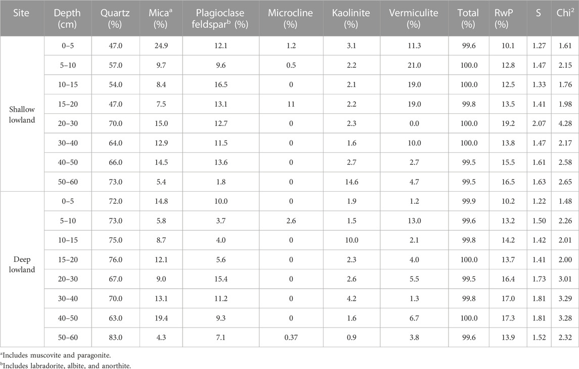
TABLE 3. Summary of mineralogy of the shallow and deep lowland core. Model fit parameters are represented by residual whole pattern (RwP), chi square (Chi2), and goodness of fit (S) as fit by Rigaku’s PDXL 2 software.
Redox potential in surface soils (≤8 cm) was on average highly oxidizing (>300 eV) in the upland (753 ± 79 mV std. dev.) but moderately oxidizing in the shallow lowland (369 ± 49 mV) and reducing in the deep lowland (198 ± 37 mV) (Figures 3, 4). On average across the study period for surface soils, Eh was significantly higher in the upland compared to the shallow lowland (p < 0.001) and the deep lowland (p < 0.001), and in the shallow lowland compared to the deep lowland (p = 0.012). Average Eh at ≥ 10 cm depth in the upland (748 ± 54 mV) and deep lowland (453 ± 72 mV) were oxidizing but varied between oxidizing and reducing conditions in the shallow lowland (334 ± 125 mV). Average Eh at depth was significantly higher in the upland compared to the shallow lowland (p = 0.002) and deep lowland (p = 0.012) but was not significantly different between the shallow and deep lowland.
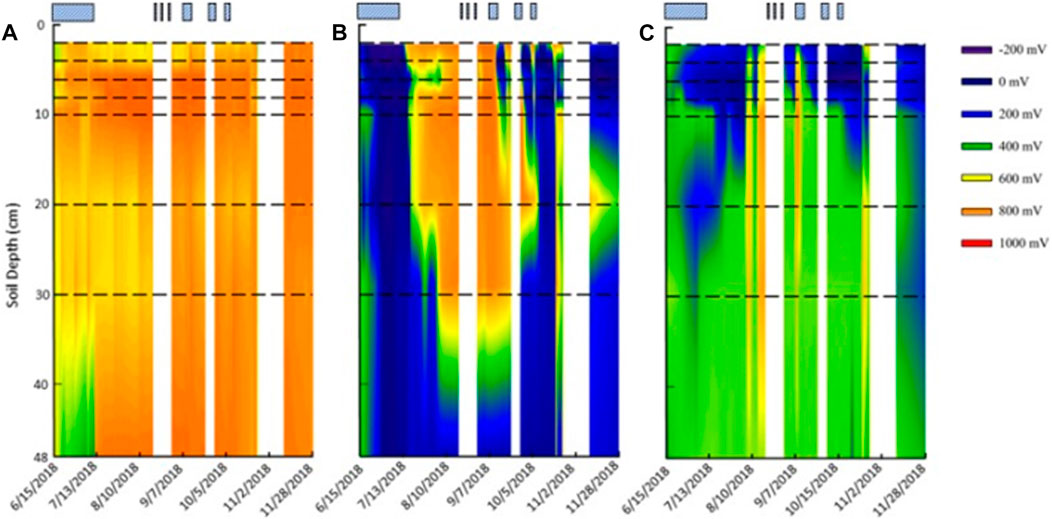
FIGURE 3. Redox probe contour maps from (A) upland, (B) shallow lowland, and (C) deep lowland. No data were recorded for the first 2 cm. Horizontal black dashed lines represent location of the eight platinum sensors on the redox probe. Striped, blue boxes represent the time the pond was flooded. White areas represent times during which no data was recorded. Maps were created with SigmaPlot 13.0.0.83.
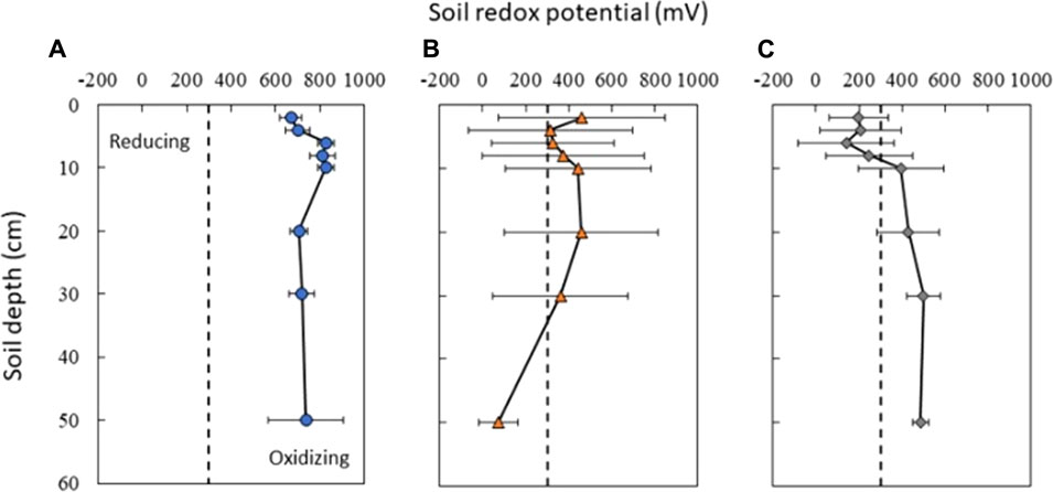
FIGURE 4. Average soil redox conditions in (A) upland (blue circles), (B) shallow lowland (orange triangles), and (C) deep lowland (grey diamonds) from June 15th to 18th October 2018. Upland soils show little variability in soil redox potential while both shallow and deep lowland soils show high variability in the surface and less variability at depth. Dotted black bar represents the 300 mV threshold between Fe reducing and oxidizing conditions. Error bars represent the standard deviation in redox potential across the study period.
Across the study period, upland soil Eh was the least variable (standard deviation <50 mV for surface soils ≤8 cm depth; std. dev. 36–169 mV for soils ≥10 cm depth). Upland soil Eh at most depths was generally stable but experienced transient increases in Eh that only lasted for a few days and that co-occurred with transient peaks in soil moisture during and immediately following rain events (Figure 5). Only one sustained major shift in Eh occurred in upland soils: at the deepest sensor location, 48 cm below the soil surface, Eh transitioned from ∼400 mV to ∼800 mV in mid-July and remained stable at 800 mV for the remainder of the data collection period. Redox potentials in lowland soils experienced greater variability than upland soils. The standard deviation in Eh at each depth ranged from 285 to 389 mV for soils ≤8 cm depth and from 90 to 359 mV for soils ≥10 cm depth in the shallow lowland, and from 136 to 224 mV for soils ≤8 cm depth and 37–200 mV for soils ≥10 cm depth in the deep lowland. These large ranges are due to major shifts in redox conditions that occurred throughout the soil profiles, concurrent with changes in surface water depth, inundation status, and soil moisture conditions described below.
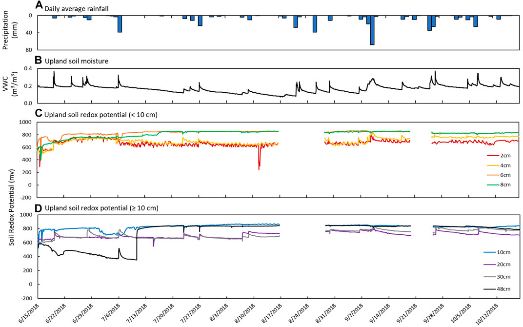
FIGURE 5. Sensor measurements from June 15th to October 18th in the upland soil. (A) Daily average precipitation, (B) soil moisture measured as volumetric water content (VWC), and soil redox potential (Eh) recorded at depths of (C) 2 cm (red), 4 cm (yellow), 6 cm (orange), and 8 cm (green) and (D) 10 cm (blue), 20 cm (purple), 30 cm (gray), and 48 cm (black).
Upland Eh remained oxidizing through time and at all depths (Figure 4A). Significantly higher average soil redox conditions were observed at 6, 8, and 10 cm depth (830 ± 38, 811 ± 57, and 826 ± 36 mV; respectively) relative to lower, but still oxidizing, Eh values recorded at 2 cm (670 ± 49 mV), 4 cm (700 ± 55 mV) and >10 cm (20 cm: 707 ± 39 mV; 30 cm: 719 ± 58 mV; 48 cm: 738 ± 169 mV) (p < 0.001). Variation in redox potential was small at all depths (±63 mV), with the highest variability observed at 48 cm (±169 mV) (Figure 4A).
Soil Eh recorded increases in soil redox potential that coincided with increases in soil moisture content and precipitation (Figure 5). For example, there were sharp increases in Eh at 2 and 4 cm depths on June 19th (+150 mV within 1 h) that corresponded to increases in soil moisture (+0.198 m3 m−3) and rainfall (6.35 mm). Similar trends were observed on July 26th and September 9th. At 20 and 30 cm, periodic increases in soil redox potential (+50–120 mV) over short periods (3–6 h) were also observed to coincide with increases in soil moisture and precipitation events. These increases in soil redox potential were usually followed by a slow trailing decrease to pre-event levels, similar to soil moisture content.
Soil Eh at 6, 8, and 10 cm depths did not respond to individual rain events but steadily increased through June before leveling off at high values during a period of low to no precipitation that coincided with a steady decrease in soil moisture content. At 48 cm depth, soil redox potential started out at the lowest levels recorded in the upland (<600 mV) and decreased over time until increasing from 350 mV to 770 mV in only 3 hours on July 10th. Soil redox potential stayed high and similar to the other depths for the remainder of the study period (Figure 5).
Redox potential in the shallow lowland was Fe reducing over the entire soil profile during early summer when the pond was flooded (Figure 4B). Redox potential then transitioned to oxidizing conditions in the top 30 cm after surface water in the shallow lowland dried out on July 9th (Figure 6). Starting July 11th, soils shifted from reducing to oxidizing conditions at different times for different depths, with deeper soils generally shifting later than shallower soils. The shift from reducing to oxidizing conditions is as follows for each depth: 2 cm (on July 13th, +4 days delay), 4 cm (+5 days), 8 and 10 cm (+6 days), 20 cm (+7 days), 6 cm (+8 days), and finally 30 cm (+15 days) (Table 4). Redox conditions at 48 cm remained reducing over the study period. Similar sequences of redox transitions were observed during subsequent shifts from flooded to dry conditions that occurred in the fall (Figure 6).
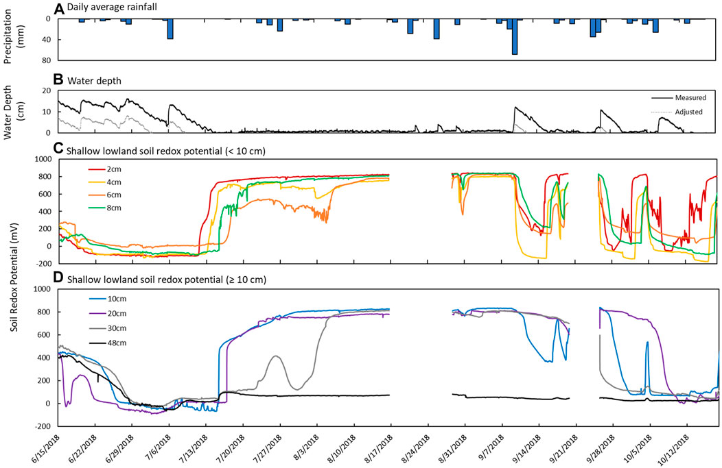
FIGURE 6. Sensor measurements from June 15th to October 18th in the shallow lowland. (A) Daily average precipitation, (B) measured water depth measured at site 12 in the deep part of the pond (solid line) and adjusted calculated water depth in the shallow lowland (dotted line), (C) estimated water depth at the redox probe in shallow part of the pond, and soil redox potential (Eh) recorded at depths of (C) 2 cm (red), 4 cm (yellow), 6 cm (orange), and 8 cm (green) and (D) 10 cm (blue), 20 cm (purple), 30 cm (gray), and 48 cm (black).
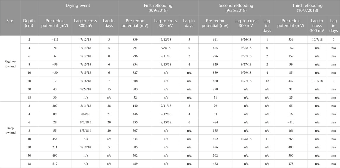
TABLE 4. Time (days) until soil redox potential crossed 300 mV during either drying or reflooding event. The drying event occurred 7/9/18 in the shallow lowland and on 7/14/18 in the deep lowland.
Redox shifts from oxidizing to reducing conditions occurred three times starting in September, with shifts to reducing conditions lasting 4 days (September 11th to 15th), 5 days (September 26th to October 1st) and 6 days (October 7th to 12th) (Figure 6). The development of reducing conditions recorded in the shallow lowland coincided with water depth increases of at least 7 cm after major precipitation events. The first shift to reducing conditions occurred at the largest increase in water depth (12 cm) and longest duration of flooding (6 days) but was also associated with the higher Eh and faster return to oxidizing conditions (overall 4 days of reducing conditions) compared to the two following events. Each subsequent redox shift resulted in lower and more reducing Eh (Figure 6). Transitions from reducing to oxidizing conditions were preceded by periods of low precipitation and decreasing soil moisture in the upland, while the transition back to reducing conditions was preceded by precipitation and increases in water depth.
Soil Eh in the deep lowland was initially oxidizing from the surface to 20 cm but transitioned to reducing conditions after 15 days where it remained for the majority of the study period with only brief periods of oxidizing conditions (Figure 4C). We can’t exclude the possibility that the initial oxidizing conditions are a result of the installation of the redox probe itself, as we also observed an initial decrease of redox potential in the shallow lowland. Similar to the shallow lowland, oxidizing conditions were preceded by periods of low precipitation and negligible surface water while reducing conditions were preceded by precipitation and increases in surface water. In contrast to the shallow lowland, soil Eh in the deep lowland was highest at 30 and 48 cm (500 ± 77 and 486 ± 37 mV, respectively), and generally decreased towards the soil surface. Average Eh in the shallow soils (199 ± 43 mV) was significantly lower than average Eh in deeper soils (453 ± 49 mV) (p < 0.001). Eh variability was highest in shallow soils and decreased with depth (Figure 7).
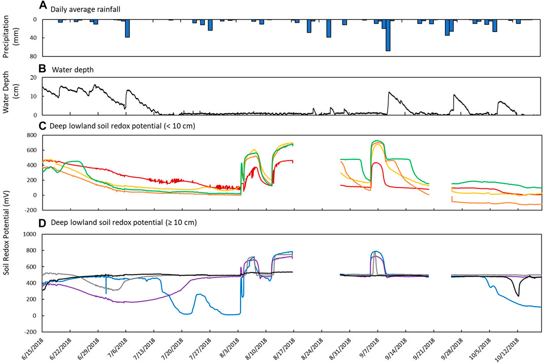
FIGURE 7. Sensor measurements from June 15th to October 18th in the deep lowland. (A) Daily average precipitation, (B) measured water depth measured at site 12 in the deep part of the pond, and soil redox potential (Eh) recorded at depths of (C) 2 cm (red), 4 cm (yellow), 6 cm (orange), and 8 cm (green) and (D) 10 cm (blue), 20 cm (purple), 30 cm (gray), and 48 cm (black).
Redox potential in the shallow soils was initially reducing but rapidly increased to oxidizing conditions over a 10-h period on August 4th, which was 24 days after surface water dried out. Unlike in the shallow lowland, Eh at the 4, 6, and 8 cm depths increased simultaneously while there was a 2 day delay before soils at 2 cm depth reached Eh >300 mV. Following ponding of surface water in early September, Eh decreased and remained reducing (Table 4). Eh remained reducing during subsequent drying and rewetting events, and further changes in water depth seemed to have no impact on Eh. Soils from 10 to 30 cm followed the same trends as the shallower soils but were generally more oxidizing throughout the study period, with each depth experiencing transient reducing conditions during wetter periods. Soil Eh at 48 cm remained stable at approximately 400, 500 mV throughout the study period.
Iron paint loss from IRIS tubes ranged from a 10.1% in the upland (Site 6) to 47.2% in the deep lowland (Site 16) (Figure 8; Supplementary Table S3). On average, the four tubes placed in the upland lost 19.1% ± 4.5% of the Fe-paint while the four tubes placed in the lowland lost 28.3% ± 8.2% of the Fe-paint. A value of higher than 25% Fe-paint removed indicates Fe reducing conditions while a range of 10%–25% Fe-paint removed indicates only potential Fe reduction (Rabenhorst, 2008).
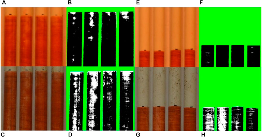
FIGURE 8. Example color photographs (A, C, E, and G) and corresponding black and white contrast images (B,D,F, and H) of IRIS probes inserted in the top 10 cm of sediments in the shallow lowland [probe 1; (A–D)] and deep lowland [probe 2; (E–H)]. Surface water was absent at the time of insertion, but pond sediments were still saturated. Top images show the probes pre-deployment and bottom images show the probes after 2 weeks incubation. Each side of each probe is shown. The calculated values in Fe loss for all probes can be found in Suplementary Table S2.
Dissolved total Fe and SRP concentrations were measured as indicators of Eh conditions in the lowland and upland soil pore waters and in the pond surface water. Across all dates and sites for which both solute concentrations and Eh values were available, shallow soil Eh (≤8 cm depth) was negatively correlated with dissolved Fe (ρ = −0.67; p = 0.009) and SRP (ρ = −0.76; p = 0.002) but not Al, Mn, Mg, Ca, or DOC concentrations. In the lowland, porewater Fe concentrations were ≥5 mg L−1 in May and June during flooded conditions in the pond, decreased to 2.1–2.5 mg L−1 in early July, and were ≤0.3 mg L−1 after July 19 when no surface water was present (Figure 9). Porewater SRP concentrations were directly correlated with Fe in the lowland (R2 = 0.99 and p < 0.001; Figure 10) and ranged from 0.09 to 0.15 mg L−1 in May and June and decreased to <0.05 mg L−1 in July. Soluble reactive P comprised most or all of total dissolved P (Figure 9). In comparison, dissolved Ca, Mg, and Mn were relatively low when the pond was flooded and then increased during the dry period. In the upland, porewater Fe was consistently <1.5 mg L−1 Fe and SRP was <0.02 mg L−1. Dissolved Ca, Mg, and Mn were also low in the upland relative to the lowland. Dissolved Al concentrations were similar in lowland and upland porewaters and decreased as the soils dried. No porewater could be collected on (for the upland) and/or after (for the lowland) July 26th (Figure 11).
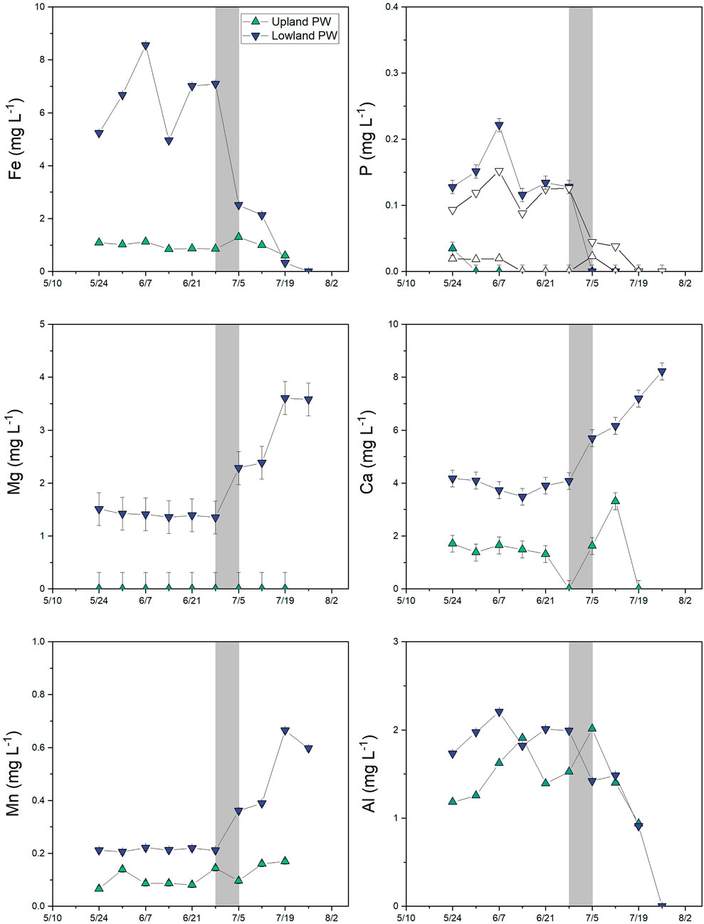
FIGURE 9. Major dissolved element concentrations (<0.45 μm) in porewater in the upland (green up triangles) and lowland (purple down triangles) from 10th May 2018 to 26 July 2018. White triangles in the phosphorus panel represent soluble-reactive P, which sometimes exceeds total dissolved P concentrations at low concentrations due to differences in detection limits. Note the difference in scale for each element. Error bars represents analytical error. Values that were below detection are plotted at zero.
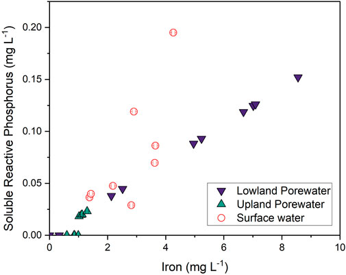
FIGURE 10. Linear regression of soluble-reactive phosphorus versus dissolved Fe in the lowland (purple down triangles; R2 = 0.99 and p < 0.001), upland (green up triangles; R2 = 0.63 and p = 0.006), and surface water (open circles; R2 = 0.46 and p = 0.04).
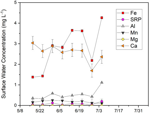
FIGURE 11. Concentrations of dissolved major elements (<0.45 μm) in the surface water from 17th May 2018, to 5th July 2018. Error bars represent analytical error. No surface water was present by mid-July.
Surface water was collected between May 10 and July 5 when the pond was still flooded. Dissolved Fe concentrations were lower in surface water (2.8 ± 1.1 mg L−1) than in lowland porewater (4.5 ± 3.0 mg L−1) and increased from 1.4 to 4.3 mg L−1 during this time (Figure 11). SRP concentrations (0.19 ± 0.11 mg L−1) were higher than in lowland porewater (0.09 ± 0.09 mg L−1) and increased from 0.04 to 0.20 mg L−1. SRP in surface water was moderately correlated with Fe (R2 = 0.46; p = 0.03) but strongly correlated with dissolved Al (R2 = 0.89; p < 0.001), which had lower concentrations (0.53 ± 0.25 mg L−1) than measured in upland and lowland porewaters (1.51 ± 0.52 mg L−1). Concentrations of other elements were relatively stable and either lower than (Ca, Mg) or similar to (Mn) porewater concentrations in the lowland over the same time period.
Soil Eh is an important indicator of potential biogeochemical processes and element cycling. Determining the direction and magnitude of Eh changes and the timeframes over which they occur in response to hydrologic change are therefore critical in understanding element cycling. Here, we determined that soil Eh across the vernal pond had variable response to changes in water depth, with Eh in the shallow lowland increasing to oxidizing conditions faster than the deeper lowland after drying of surface water. Furthermore, redox potential exhibited lag times of days to weeks following drying and rewetting, indicating that the presence of surface water is not necessarily a good reflection of redox conditions in underlying soils.
We observed two different hydrologic scenarios resulting in fluctuating soil redox conditions. The first scenario is the drying of surface water in the vernal pond during times of prolonged warm temperatures and low precipitation in summer. The second scenario represents intermittent reflooding of the vernal pond during late summer and early autumn as temperatures decrease and precipitation increases.
The presence or absence of surface water or soil saturation alone was not a good indicator of soil Eh in either lowland position. Much like a solution with a high acid buffering capacity can resist a change in pH with addition of acid, ecological systems can resist a change in Eh through a disturbance. The redox buffer capacity of a system can be indicated by the lag time needed to observe a change in Eh following a disturbance and can have many causes (Burgin and Loecke, 2023). For example, decreases in Eh following saturation will not occur until O2 is consumed, thus lag times depend in part on the concentrations of redox-active species. Redox buffering may also occur due to physical factors that influence water and solute retention and movement through a system.
Variability in the response of soil Eh to decreases in soil saturation in our system may be explained by soil pores still being partially saturated and drying out over time. Dorau et al. (2018a) describe that Eh increases as the air-filled pore volume of soil increases. While soil Eh in both the shallow and deep subsurface were reducing during flooded conditions, the transition to oxic conditions once surface water dried out was delayed. This delay of the response of soil Eh to hydrological change was shorter in the shallow lowland (3–15 days) compared to the deep lowland (20–28 days) (Table 4). D’Amore et al. (2004) observed a time lag of 14–19 days between when wetland soils became saturated and when Fe-reducing conditions developed, which although documenting the opposite hydrologic and redox shift, agrees well with the occurrence of time lags observed in this study. Other authors reported an Eh increase of about 540 mV within 24 h after aeration as the water table declines in marsh soils at 10 cm depth, similar to the magnitude of Eh increase observed in the shallow and deep lowland soils (Dorau and Mansfeldt, 2016). Increases in redox potential in the upland were consistent with decreases in soil moisture. Redox potential peaked in June and stabilized around 700 mV despite soil moisture decreasing further. Redox potential can fluctuate between −300 and 900 mV in natural soils (Macías and Arbestain, 2010), and the measured value of Eh could indicate a stable level for the upland soil during the end of summer independent of declining soil moisture. The observed spatially and temporally heterogenous Eh and lags in changes of Eh following hydrologic change could be influenced by differences in soil composition, drainage, evapotranspiration, microbial activity, and/or changes to microbial activity and root respiration (Rubol et al., 2012; Peralta et al., 2014). Surface water depth is likely not a determining factor in describing the difference in Eh lag time between the shallow and deep lowland as the deep lowland dried out just a week after the shallow lowland but didn’t transition to oxic condition for a further 3 weeks. Retention of pore water is likely the cause of the increased delay in the deep lowland. For example, a clay-rich layer will retain porewater longer than a sandy soil, potentially increasing the lag time between the drying up of surface water and an increase in soil redox potential. In fact, there was a noticeable difference between the shallow and deep lowland by the end of July with the deep lowland being muddy while the shallow lowland was indistinguishable from the upland. Partially this could be explained with the deep lowland being the topographic low and receiving drainage from the shallow lowland and the surrounding upland especially after any precipitation event, but very little precipitation was recorded during this time period.
Although we did not measure soil moisture in the lowland in this study, soil texture may provide insights on the potential for these soils to retain water. Although the clay and silt size fractions were similar from 5 to 60 cm between the shallow (48% ± 6%) and the deep (46% ± 12%) areas of the pond, clay minerals quantified by XRD were higher in the shallow lowland (average 14.2% ± 8.2%) than the deep lowland (8.3% ± 3.9%), particularly in surface soils. Clays in the shallow lowland were dominated by vermiculite, with the exception of a kaolinite-rich layer from 50 to 60 cm depth, while the deep lowland was dominated by kaolinite. Dorau et al. (2018a) describes how air-filled pore volume impacts soil Eh, and how contact of redox potential measurement by Pt electrodes are impacted by distribution of soil particles. In short, the larger the pore space in a soil, the lower the required air-filled pore volume needed to achieve oxidizing soil redox conditions. In soils with small pore spaces, water is retained around the Pt electrode and a higher air-filled pore volume is required to allow access to O2 to the sensor. While air-filled pore volume and pore-size distribution were not measured in this study, higher concentrations of vermiculite could result in larger pores in the shallow lowland when dry compared to the kaolinite-dominated deep lowland. Soil redox conditions could increase faster in a more porous soil, as described in Dorau et al. (2018a). D’Amore et al. (2004) come to similar conclusion with swelling clays allowing eased entry of water during unsaturated conditions.
Additionally, vermiculite is a 2:1 phyllosilicate swelling clay containing an interlayer space providing it with a large cation exchange capacity and water retaining capacity. Kaolinite, a 1:1 phyllosilicate, has a lower cation exchange capacity and water retaining capacity (Gaiser et al., 2000; Kome et al., 2019). While this would suggest that the shallow lowland should retain water longer, this could explain why it dries out first. Many studies have shown that plants and microorganisms have easier access to needed nutrients, such as K+, in 2:1 clays, like vermiculite compared to 1:1 clays like kaolinite (Ransom et al., 1999; Chorover et al., 2007; Cuadros, 2017). Cuadros (2017) notes that smectite (another 2:1 phyllosilicate) for example, is more nutrient-rich than kaolinite and microorganisms in kaolinite-rich environments would have to be more aggressive in order to obtain the same nutrients compared to a smectite-rich environment. The shallow lowland could therefore be more attractive for plant roots to grow in and experience higher evapotranspiration as a result.
Furthermore, while Eh is expected to increase first at the surface following drying due to oxygen diffusing downwards and evaporation being higher at the surface, Eh in the shallow lowland remained more reducing near the surface (at 4 and 6 cm) than slightly deeper in the soil profile (at 8 and 10 cm), which may indicate higher microbial activity at those depths. Microorganisms lower soil redox potential by consuming oxygen more rapidly than it is replenished by diffusion, particularly in saturated and flooded soils, and by consuming other terminal electron acceptors during microbial respiration and decomposition (Husson, 2013). Therefore, continued microbial decomposition of organic material in the shallow lowland in combination with soil moisture retention could explain the 1-week delay between the pond drying out and rising redox potential.
On average, both the shallow and deep lowland were oxidizing (>300 mV) below 10 cm depth, except for the shallow lowland at 48 cm. This is despite the expectation laid out above that deeper soils would be more reducing given than oxygen has a longer diffusion path and would be consumed by microorganism in shallow soils. Water flow paths and/or lower microbial activity could explain why Eh is higher with depth, as has been observed in other studies (Dorau et al., 2021; Thomas et al., 2009; D’Amore et al., 2004). Relatively oxidizing conditions at depth may be explained by lateral flow paths that allow for the influx of oxygenated water into the subsurface (D’Amore et al., 2004). Additionally, low soil carbon content at depth in both shallow and deep lowland could limit aerobic respiration and therefore the consumption of O2. Connectivity of soil pores can also be an important determining factor in Eh. The consistent reducing conditions at 48 cm depth in the shallow lowland can be explained by an underlying kaolinite clay-rich layer (50–60 cm depth) that restricts drainage and allows water to pond (Kome et al., 2019). While water table depth was not measured through the study period, it was at about 30 cm below the soil surface when the soil core was removed in October. Additional evidence for the occurrence of the water table above 30 cm depth can be inferred from Eh conditions. Eh at 30 cm lagged behind the Eh increases closer to the surface following drying and then decreased again for a time period after heavy precipitation, indicating re-saturation.
The second scenario observed was intermittent flooding and soil rewetting that drove returns to reducing conditions in the lowland during times of increased precipitation and decreasing temperatures. Like in the first scenario, Eh in the shallow lowland was more sensitive to changes in water depth than the deep lowland, indicated by the faster change towards oxidizing condition after drying of surface water and by rapid fluctuations between reducing and oxidizing conditions following three major precipitation events. In comparison, the deep lowland returned to reducing conditions following the first rain event and remained reducing during subsequent dry periods. It is therefore likely that the soil only became unsaturated enough to be oxidizing during the extended dry period in early summer. During the first major precipitation event in September, pores saturated with water and remained saturated, causing reducing conditions to develop in the deep lowland despite no surface water.
The steplike pattern (Figure 7) observed in the surface soils of the deep lowland during the first reflooding event in early September provides more insight to the disconnect of Eh and water depth in the deep lowland. Specifically, each depth remained poised at a particular Eh for a period of time before rapidly decreasing. Dorau et al. (2021) attributed a similar trend to pore connectivity. If pores are well connected, aeration or saturation of pores results in either an increase or decrease in Eh, respectively. If pores are not well connected, the diffusion of O2 might be limited and equal to O2 consumption, causing stable Eh conditions for a period of time until a moisture threshold is reached. As a result, Eh was stable until pores were sufficiently saturated, and subsequent precipitation and reflooding events had no impact on Eh given that poorly connected pores would retain moisture after surface water dried out. We only observe these step pattern in the deep lowland but not in the shallow lowland. Therefore, it is likely that the deep lowland has low pore connectivity while the shallow lowland has higher pore connectivity.
Porewater Fe concentrations were up to 10× higher in the lowland when it was flooded than when there was no surface water. This result indicates that the reducing conditions in the lowland promoted the reduction of Fe-oxides during flooded conditions and the removal of Fe in the porewater through precipitation of Fe-oxides as drying shifted the soils towards oxidizing conditions. As porewater was combined from both the shallow and deep site of the pond, it could not be determined if the longer reducing conditions in the deep lowland also resulted in higher Fe concentrations in the porewater. Dissolved Fe concentrations declined over the time between when surface water dried and when deep lowland soils became oxidizing, possibly reflecting the combination of low Fe water from more oxidizing areas and high Fe water from more reducing areas of the pond.
Similar to trends for Fe, porewater SRP concentrations in the lowland were >2× higher during flooded periods than dry periods. Given that phosphate strongly associates with Fe oxides in soils and sediments (Ruttenberg and Sulak, 2011), we attribute this pattern to the release of phosphate into solution during flooded, reducing conditions and subsequent sorption to Fe oxides during dry, oxidizing conditions. The linear correlation of SRP with soluble Fe in the lowland (Figure 10; r2 = 0.99 and p < 0.001) strongly supports this assumption. Increases in Fe and SRP in surface water from May to early July also reflect reducing conditions in the underlying soils and solute release into the overlying water. SRP was very strongly correlated with dissolved Fe in lowland porewaters but only weakly correlated in surface waters, where a stronger correlation with dissolved Al was observed. Possibly Al is also released through reductive dissolution of Fe-oxide minerals, or potentially SRP that is released from Fe-oxide minerals in soils becomes associated with filterable Al colloids in the surface water (Khare et al., 2005). Iron and SRP concentrations in the upland soils were consistently low and similar to concentrations observed in the lowland during the dry period.
Unlike patterns observed for Fe, P, and Al, concentrations of Ca, Mg, and Mn increased over time in lowland porewaters following the drying of surface water. Although Mn is redox sensitive and would be expected to follow patterns for Fe, it is also more stable in solution and can persist under oxidizing conditions (Yazbek et al., 2021). Mn may instead follow patterns for Ca and Mg if it is derived from a similar source, for example, from deeper subsurface water. As the surface soil dries, it is possible that capillary action brings deeper water close to the surface and affects solution chemistry (Ronen et al., 2000). Alternatively, it is possible that these elements are enriched through evaporative concentration.
Iron loss from the IRIS tubes was consistent with recorded redox conditions. The four IRIS tube placed in the lowland indicated a definitive reducing environment with more than 25% of the paint lost, while the four tubes placed in the upland were more consistent with a probable reducing environment (10%–25% loss) (Rabenhorst, 2008). The 9% difference between the upland and lowland probes can be taken as an indication that the lowland is more reducing and conducive for Fe oxide reduction than the upland (Rabenhorst, 2008). In the upland, periodic anoxia driven by rainfall events and localized anoxic conditions could explain Fe loss. Abrasion during the insertion and removal of the IRIS tubes could also explain some loss of Fe paint. Differences in IRIS Fe loss between the shallow and deep lowland were also consistent with differences in redox potential. IRIS tube 1 was placed in the shallow lowland and recorded a Fe-paint loss of 16.8% while the remaining three IRIS tubes were placed in the more reducing deep lowland recorded an average Fe-paint loss of 33.9% ± 10.8%. Since IRIS tubes record an integrated signal over time, we cannot determine whether Fe loss occurred within the first week of placement or over the entire 2 weeks.
These are important findings in context of geochemical cycling of elements like Fe and P. Previous studies have suggested that the formation of redoximorphic features not only depend on reducing condition but on the duration of reducing conditions (Vepraskas, 2015; Dorau et al., 2018b). Development of reducing conditions that drive Fe and P geochemistry will therefore be dependent not only on the reflooding of the vernal pond itself will therefore have less importance to geochemical cycling of elements than the steady increase of the water table but also on sediment properties that influence pore saturation, antecedent moisture conditions, and lateral inflows of water.
In this study, we have shown that redox potential in soils varies with time and space and has variable response to water depth in a vernal pond. We confirmed our hypothesis that the dynamic hydrological condition in the lowland results in dynamic Eh conditions compared to the hydrological static upland. Additionally, Fe and SRP were higher during flooded pond conditions confirming our third hypothesis. The strong correlation of Fe and SRP (r2 = 0.99 and p < 0.001) in the flooded lowland reinforces the importance of soil Eh on important biogeochemical cycling of vital elements to the environment such as P. We did not confirm our hypothesis that Eh would decrease with depth, attributed to the presence of a more oxidizing subsurface layer, but did show that Eh is less variable in deeper soils. In summer as the vernal pond dried out, increases in redox potential associated with oxygenation lagged behind disappearance of surface water by up to weeks, with lag times that differed across the pond and with depth. In contrast, each reflooding event of the vernal pond in the fall almost immediately led to decreases in redox potential with longer durations of reducing conditions with each subsequent reflooding. We contend that a vernal pond cannot be viewed as a homogeneous redox environment, but as a heterogeneous environment where reducing and oxidizing conditions spatially coexist and vary with time. As such, predicting the geochemical cycling of elements based on changing redox conditions in response to flooding or drying depends on many factors such as microbial activity, redox buffering capacity of the soil, and/or the time it takes for the soil to wet or dry. The factors in return depend on physical properties of the soil such as soil composition, pore structure or the amount of organic matter. Relying only on hydrological factors such as surface water and soil moisture will not produce accurate predictions of Eh and therefore may misrepresent biogeological cycling of elements such as Fe and P.
These findings become more important when taking into context of climatic change and shifting precipitation patterns. Prolonged dry spells followed by more intense precipitation events will impact the duration of surface water ponding and numbers of reflooding events. Persistently dry conditions result in long oxidizing periods in the summer and more redox fluctuations in the fall that will impact microbial activity and geochemical cycling of elements. Further studies into these processes combined with the observation of important geochemical cycling of elements related to redox potentials, such as N, C, and Fe, will provide further insight into the importance of environments with fluctuating hydrology and Eh.
The raw data supporting the conclusion of this article will be made available by the authors, without undue reservation.
MB performed the analysis, redox data collection and prepared the manuscript. MB, CS, and ND performed field and lab work. ND created the pond map with ArcGIS. All authors contributed to the article and approved the submitted version.
This work was supported by grants from the National Science Foundation (EAR-1609027 and OPP-2006194) and the Kent State Environmental Science and Design Research Initiative to EH and LK-C.
We would like to thank Shannon Joseph, Devin Starr and Emily Mehta for field and lab work assistance.
The authors declare that the research was conducted in the absence of any commercial or financial relationships that could be construed as a potential conflict of interest.
All claims expressed in this article are solely those of the authors and do not necessarily represent those of their affiliated organizations, or those of the publisher, the editors and the reviewers. Any product that may be evaluated in this article, or claim that may be made by its manufacturer, is not guaranteed or endorsed by the publisher.
The Supplementary Material for this article can be found online at: https://www.frontiersin.org/articles/10.3389/fenvs.2023.1114814/full#supplementary-material
Bauder, E. T. (2005). The effects of an unpredictable precipitation regime on vernal pool hydrology. Freshw. Biol. 50, 2129–2135. doi:10.1111/j.1365-2427.2005.01471.x
Blackwood, C. B., Smemo, K. A., Kershner, M. W., Feinstein, L. M., and Valverde-Barrantes, O. J. (2013). Decay of ecosystem differences and decoupling of tree community–soil environment relationships at ecotones. Ecol. Monogr. 83 (3), 403–417. doi:10.1890/12-1513.1
Burgin, A. J., and Loecke, T. D. (2023). The biogeochemical redox paradox: How can we make a foundational concept more predictive of biogeochemical state changes?. Biogeochemistry. doi:10.1007/s10533-023-01036-9
Chorover, J., Kretzschmar, R., Garcia-Pichel, F., and Sparks, D. L. (2007). Soil biogeochemical processes within the critical zone. Elements 3, 321–326. doi:10.2113/gselements.3.5.321
Cogger, C. G., Kennedy, P. E., and Carlson, D. (1992). Seasonally saturated soils in the Puget lowland II. measuring and interpreting redox potentials. Soil Sci. 154, 50–58. doi:10.1097/00010694-199207000-00007
Colburn, E. A. (2004). Vernal pools: Natural history and conservation. Granville, OH: The McDonald and Woodward Publishing Company, 426.
Cuadros, J. (2017). Clay minerals interaction with microorganisms: A review. Clay Miner. 52, 235–261. doi:10.1180/claymin.2017.052.2.05
D’Amore, D. V., Stewart, S. R., and Huddleston, J. H. (2004). Saturation, reduction, and the formation of iron–manganese concretions in the jackson-frazier wetland, Oregon. Soil scie. Soc. Am. J. 68, 1012–1022. doi:10.2136/sssaj2004.1012
Dorau, K., Wessel-Bothe, S., Milbert, G., Schrey, H. P., Elhaus, D., and Mansfeldt, T. (2018b). Climate change and redoximorphosis in a soil with stagnic properties. Catena 190, 104528. doi:10.1016/j.catena.2020.104528
Dorau, K., Bohn, B., Weihermüller, L., and Mansfeldt, T. (2021). Temperature-induced diurnal redox potential in soil. Environ. Sci. Process. Impacts 23, 1782–1790. doi:10.1039/d1em00254f
Dorau, K., Luster, J., and Mansfeldt, T. (2018a). Soil aeration: The relation between air-filled pore volume and redox potential. Eur. J. Soil Sci. 69 (6), 1035–1043. doi:10.1111/ejss.12717
Dorau, K., and Mansfeldt, T. (2016). Comparison of redox potential dynamics in a diked marsh soil: 1990 to 1993 versus 2011 to 2014. J. Plant Nutr. Soil Sci. 179, 641–651. doi:10.1002/jpln.201600060
Fiedler, S., and Sommer, M. (2004). Water and redox conditions in wetland soils-their influence on pedogenic oxides and morphology. Soil Sci. Soc. Am. J. 68 (1), 326–335. doi:10.2136/sssaj2004.3260
Fiedler, S., Vepraskas, M. J., and Richardson, J. (2007). Soil redox potential: Importance, field measurements, and observations. Adv. Agron. 94, 1–54. doi:10.1016/S0065-2113(06)94001-2
Gaiser, T., Graef, F., and Cordeiro, J. C. (2000). Water retention characteristics of soils with contrasting clay mineral composition in semi-arid tropical regions. Aust. J. Soil Res. 38, 523–536. doi:10.1071/sr99001
Glinski, J., and Stepniewski, W. (1985). Soil aeration and its role for plants. 1st. Boca Raton, FL: CRC Press.
Husson, O., Husson, B., Brunet, A., Babre, D., Alary, K., Sarthou, J. P., et al. (2016). Practical improvements in soil redox potential (Eh) measurement for characterisation of soil properties. Application for comparison of conventional and conservation agriculture cropping systems. Anal. Chim. Acta 4 (906), 98–109. doi:10.1016/j.aca.2015.11.052
Husson, O. (2013). Redox potential (Eh) and pH as drivers of soil/plant/microorganism systems: A transdisciplinary overview pointing to integrative opportunities for agronomy. Plant Soil 362, 389–417. doi:10.1007/s11104-012-1429-7
Kappler, A., Bryce, C., Mansor, M., Lueder, U., Byrne, J. M., and Swanner, E. D. (2021). An evolving view on biogeochemical cycling of iron. Nat. Rev. Microbiol. 19, 360–374. doi:10.1038/s41579-020-00502-7
Khare, N., Hesterberg, D., and Martin, J. D. (2005). XANES investigation of phosphate sorption in single and binary systems of iron and aluminum oxide minerals. Environ. Sci. Technol. 39 (7), 2152–2160. doi:10.1021/es049237b
Kome, G., Enang, R. K., Tabi, F., and Yerima, B. (2019). Influence of clay minerals on some soil fertility attributes: A review. Open J. Soil Sci. 09, 155–188. doi:10.4236/ojss.2019.99010
LaRowe, D. E., and Van Cappellen, P. (2011). Degradation of natural organic matter: A thermodynamic analysis. Geochimica Cosmochimica Acta 75, 2030–2042. doi:10.1016/j.gca.2011.01.020
Macías, F., and Arbestain, M. C. (2010). Soil carbon sequestration in a changing global environment. Mitig. Adapt. Strateg. Glob. Change 15, 511–529. doi:10.1007/s11027-010-9231-4
Mansfeldt, T. (2003). In situ long-term redox potential measurements in a dyked marsh soil. J. Plant Nutr. Soil Sci. 166, 210–219. doi:10.1002/jpln.200390031
Mansfeldt, T., and Overesch, M. (2013). Arsenic mobility and speciation in a gleysol with petrogleyic properties: A field and laboratory approach. Heavy Metal Environ. 42 (4), 1130–1141. doi:10.2134/jeq2012.0225
Mansfeldt, T. (2004). Redox potential of bulk soil and soil solution concentration of nitrate, manganese, iron, and sulfate in two gleysols. J. Plant Nutr. Soil Sc. 167, 7–16. doi:10.1002/jpln.200321204
Markelova, E. (2017). “Redox potential and mobility of contaminant oxyanions (as, Sb, Cr) in argillaceous rock during oxic and anoxic cycles,”. PhD (Canada: University of Waterloo).
McClain, M. E., Boyer, E. W., Dent, C. L., Gergel, S. E., Grimm, N. B., Groffman, P. M., et al. (2003). Biogeochemical hot spots and hot moments at the interface of terrestrial and aquatic ecosystems. Ecosystems 6, 301–312. doi:10.1007/s10021-003-0161-9
Murphy, J., and Riley, J. P. (1962). A modified single solution method for the determination of phosphate in natural waters. Analytica Chimica Acta. 27 (C), 31–36–36. doi:10.1016/S0003-2670(00)88444-5
National Oceanic Atmospheric Agency/National Centers for Environmental Information (2021). Climate data online. Subset used 1998-2018. Available at: https://www.ncei.noaa.gov/cdo-web/(Accessed July 27, 2021).
Onset Computer Corporation (2020). HOBOware® user’s guide. Available at: https://www.onsetcomp.com/resources/documentation/12730-hoboware-users-guide.
Peralta, A. L., Ludmer, S., Matthews, J. W., and Kent, A. D. (2014). Bacterial community response to changes in soil redox potential along a moisture gradient in restored wetlands. Ecol. Eng. 73, 246–253. doi:10.1016/j.ecoleng.2014.09.047
Peretyazhko, T., and Sposito, G. (2005). Iron(III) reduction and phosphorous solubilization in humid tropical forest soils. Geochim. Cosmochim. Acta 69 (14), 3643–3652. doi:10.1016/j.gca.2005.03.045
Rabenhorst, M. C. (2008). Protocol for Using and Interpreting IRIS Tubes. Soil Survey Horizons 49 (3), 74–77. doi:10.1016/j.gca.2005.03.045
Rabenhorst, M. C., and Burch, S. N. (2006). Synthetic iron oxides as an indicator of reduction in soils (IRIS). Soil Science Society of America Journal 70 (4), 1227–1236. doi:10.2135/sssaj2005.0354
Ransom, B., Bennett, R. H., Baerwald, R., Hulbert, M. H., and Burkett, P. J. (1999). In situ conditions and interactions between microbes and minerals in fine-grained marine sediments: ATEM microfabric perspective. Am. Mineralogist 84, 183–192. doi:10.2138/am-1999-1-220
Reddy, K. R., and Delaune, R. D. (2008). Biogeochemistry of wetlands: Science and applications. Boca Raton, FL: CRC Press.
Rezanezhad, F., Couture, R.-M., Kovac, R., O’Connell, D., and Van Cappellen, P. (2014). Water table fluctuations and soil biogeochemistry: An experimental approach using an automated soil column system. J. Hydrol. 509, 245–256. doi:10.1016/j.jhydrol.2013.11.036
Rivett, M. O., Buss, S. R., Morgan, P., Smith, J. W., and Bemment, C. D. (2008). Nitrate attenuation in groundwater: A review of biogeochemical controlling processes. Water Res. 42, 4215–4232. doi:10.1016/j.watres.2008.07.020
Ronen, D., Scher, H., and Blunt, M. (2000). Field observations of a capillary fringe before and after a rainy season. J. Contam. Hydrol. 44, 103–118. doi:10.1016/s0169-7722(00)00096-6
Rubol, S., Silver, W. L., and Bellin, A. (2012). Hydrologic control on redox and nitrogen dynamics in a peatland soil. Sci. Total Environ. 432, 37–46. doi:10.1016/j.scitotenv.2012.05.073
Rühle, F. A., von Netzer, F., Lueders, T., and Stumpp, C. (2015). Response of transport parameters and sediment microbiota to water table fluctuations in laboratory columns. Vadose Zone J. 14, 1–12. doi:10.2136/vzj2014.09.0116
Ruttenberg, K. C., and Sulak, D. J. (2011). Sorption and desorption of dissolved organic phosphorus onto iron (oxyhydr)oxides in seawater. Geochim. Cosmochim. Acta 75, 4095–4112. doi:10.1016/j.gca.2010.10.033
Smith, D. W., and Verrill, W. (1998). “Vernal pool-soil-landform relationships in the central valley,” in Environmental science (Sacramento, CA: California Native Plant Society).
Street, L. E., Dean, J. F., Billett, M. F., Baxter, R., Dinsmore, K. J., Lessels, J. S., et al. (2016). Redox dynamics in the active layer of an arctic headwater catchment; examining the potential for transfer of dissolved methane from soils to stream water. Journal of Geophysical Research: Biogeosciences 121 (11), 2776–2792. doi:10.1002/2016JG003387
Thamdrup, B. (2000). “Bacterial manganese and iron reduction in aquatic sediments,” in Advances in microbial ecology (Boston, MA: Springer).
Thomas, C. R., Mia, S., and Sindhoj, E. (2009). Environmental factors affecting temporal and spatial patterns of soil redox potential in Florida Everglades wetlands. Wetlands 29, 1133–1145. doi:10.1672/08-234.1
Vepraskas, M. J. (2015). Redoximorphic features for identifying aquic conditions, technical bulletin 301. Raleigh, NC, USA: North Carolina State University.
Wallace, C. D., Sawyer, A. H., and Barnes, R. T. (2019). Spectral analysis of continuous redox data reveals geochemical dynamics near the stream–aquifer interface. Hydrol. Process. 33 (3), 405–413. doi:10.1002/hyp.13335
Wallace, C. D., and Soltanian, M. R. (2021). Underlying riparian lithology controls redox dynamics during stage-driven mixing. J. Hydrology 595, 126035. doi:10.1016/j.jhydrol.2021.126035
Yazbek, L. D., Cole, K. A., Shedleski, A., Singer, D., and Herndon, E. M. (2021). Hydrogeochemical processes limiting aqueous and colloidal Fe export in a headwater stream impaired by acid mine drainage. ACS ES&T Water 1 (1), 68–78. doi:10.1021/acsestwater.0c00002
Yu, K., Böhme, F., Rinklebe, J., Neue, H.-U., and DeLaune, R. D. (2007). Major biogeochemical processes in soils-A microcosm incubation from reducing to oxidizing conditions. Soil Sci. Soc. Am. J. 71, 1406–1417. doi:10.2136/sssaj2006.0155
Yu, K., and Patrick, W. H. (2004). Redox window with minimum global warming potential contribution from rice soils. Soil Sci. Soc. Am. J. 68 (6), 2086–2091. doi:10.2136/sssaj2004.2086
Yu, X., LeMonte, J. J., Li, J., Stuckey, J. W., Sparks, D. L., Cargill, J. G., et al. (2023). Hydrologic control on arsenic cycling at the groundwater-surface water interface of a tidal channel. Environ. Sci. Technol. 57, 222–230. doi:10.1021/acs.est.2c05930
Keywords: soil redox, redox potential, variably inundated environments, vernal ponds, hydrology
Citation: Barczok M, Smith C, Di Domenico N, Kinsman-Costello L and Herndon E (2023) Variability in soil redox response to seasonal flooding in a vernal pond. Front. Environ. Sci. 11:1114814. doi: 10.3389/fenvs.2023.1114814
Received: 02 December 2022; Accepted: 29 June 2023;
Published: 07 July 2023.
Edited by:
Xingyuan Chen, Pacific Northwest National Laboratory (DOE), United StatesReviewed by:
Axel Schippers, Federal Institute for Geosciences and Natural Resources, GermanyCopyright © 2023 Barczok, Smith, Di Domenico, Kinsman-Costello and Herndon. This is an open-access article distributed under the terms of the Creative Commons Attribution License (CC BY). The use, distribution or reproduction in other forums is permitted, provided the original author(s) and the copyright owner(s) are credited and that the original publication in this journal is cited, in accordance with accepted academic practice. No use, distribution or reproduction is permitted which does not comply with these terms.
*Correspondence: Maximilian Barczok, bWJhcmN6b2tAa2VudC5lZHU=
Disclaimer: All claims expressed in this article are solely those of the authors and do not necessarily represent those of their affiliated organizations, or those of the publisher, the editors and the reviewers. Any product that may be evaluated in this article or claim that may be made by its manufacturer is not guaranteed or endorsed by the publisher.
Research integrity at Frontiers
Learn more about the work of our research integrity team to safeguard the quality of each article we publish.