Inter-annual sea level change and transgression along a barrier Island coast

On the decadal time scale of coastal planning and management, relative sea-level rise is usually considered a trend or constant rate rather than a dynamic, time varying influence on coastal change. However, the coastal ocean sea level along the east coast of Florida and coastal regions further north is, to a first order, controlled at the interannual and decadal time scale by the dynamics of North Atlantic circulation and Gulf Stream (GS) flow, Every coastal region has its own distinctive annual sea-level cycle, and longer-term intra- and inter-decadal sea-level oscillations. This paper addresses the influence of the strong Florida coastal ocean sea-level signal on topographic evolution of the shoreface, coastal sediment budgets, and potential for coastal transgression at the decadal time scale.

1 Introduction

This analysis is facilitated by decades of semiannual spatially comprehensive topographic surveys from the top of a barrier island superstructure to a depth of −12.2 m, as prescribed in the management plan of the Sebastian Inlet Management District (SID). The survey data are from the vicinity of the Sebastian Inlet on the central Florida coast, as shown in Figure 1. The survey area extends for approximately 20 km and includes the shoals associated with the Sebastian Inlet at the center of the survey footprint. The SID was established in 1919 and was permanently stabilized by two offset jetties in the late 1940s. Semi-annual topographic surveys are based on a combination of the single-beam and multi-beam acoustic method. Topographic surveys are supplemented with an annual georeferenced aerial image survey of the areas at a spatial resolution of 0.3 m. Water level records, meteorological data, and directional wave data are also included in the SID Annual State of the Inlet Technical Reports (https://www.sitd.us/state-of-the-inlet-reports). These reports, issued since 2007, describe in detail data collection and analysis methods.

FIGURE 1

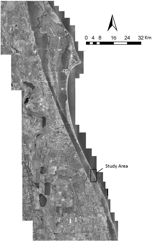
FIGURE 1. Location of the study area on the east central coast of Florida, United States.

The study area is a barrier island centered around the Sebastian Inlet, where a system of shoals has developed since the inlet was cut and stabilized. The barrier island forms the east bank of the microtidal Indian River Lagoon (Figure 1). The early history of the barrier system was influenced by numerous storm overwash events and tidal inlet breaching and migration, as evidenced by relict tidal inlet morphology now included in the barrier island. Peak elevation of the barrier island superstructure is about 8 m above mean sea level, where natural dunes still exist. The ocean tide is semidiurnal, having a mean tidal range of about 1 m. The regional wave climate is energetic, having an average significant wave height of about 0.6 m and a strong seasonal variation that includes winter nearshore wave heights of about 1 m. Storm waves in the area reach an excess of 4 m during strong tropical storms and hurricanes. It is common for two or more major tropical storms to impact the coast in any given decade. The shoreface sediment regime is a mixture of quartz-rich medium to fine sand mixed with 50% or more carbonate fraction. Carbonates are locally derived from the underlying limestone and coquina formations, and form a significant coarse fraction of barrier island shoreface sediments ranging up to the gravel size. Details of the geologic and environmental setting can be found in Zarillo et al. (2007).

2 Regional and coastal ocean sea level

Relative sea-level (RSL) rise is usually considered a trend in conceptual analysis and numerical time-marching coastal evolution models rather than a dynamic, time varying influence. Furthermore, trends of sea-level rise applied to coastal resiliency are often based on global sea level on a 50–100-year time scale projected by global climate models. Global mean sea level (GMSL) is thought to have increased at a rate of 1.5 mm yr^-1 since about 1900 (Church and White, 2011; Dangendorf et al., 2022).

Over the satellite altimetry era of 1992 to present, rates of global MSL rise have reached values of about 3 mm yr^-1. However, every coastal region has its own “fingerprint” annual sea-level cycle, and longer-term intra- and inter-decadal sea-level oscillations. A significant effort has been made to assess and refine the regional sea-level rise within the venue of GMSL predictions. In a study by Sweet et al. (2017) sponsored by NOAA, GMSL rise scenarios are integrated with regional factors to produce RSL rise responses on a 1-degree grid, covering the coastlines of the U.S. mainland, Alaska, Hawaii, the Caribbean, and the Pacific island territories. Among the regional factors considered that affect relative sea level are the sea surface height (SSH), vertical land movement (VLM) from isostatic adjustments, land–water storage, oceanographic processes (sterodynamic sea level, SDSL), tectonics, and sediment compaction. A final product of the NOAA study is gridded RSL rise predictions for the coastal regions of the U.S. that can be added to six GMSL rise scenarios that range from a minimum of 0.3 m to a maximum of 2.5 m by the year 2100.

Another recent study by Dangendorf et al. (2022) also addresses regional differences in the rate of RSL rise along the East Coast and Gulf Coast of the U.S. Plausible explanations are presented for sea-level variability and multi-year trends of observed RSL. Like the NOAA study, Dangendorf et al. (2022) recognized that the rate of RSL size has accelerated along the southeast US coast since 1992 and notably peaking in the 2010–2021 period. Through analysis of tide records and more recent satellite altimetry records, a decadal scale oscillation of southeast US coastal sea level is recognized, including sea-level peaks in the 1940s, 1970s, and in the most recent period since 2000. Although the most recent peak in RSL rise, approaching 10 mm yr^-1, if extended to 2100 m, would match NOAA’s intermediate RSL rise scenario, Dangendorf et al. (2022) suggested that the decadal oscillation will continue and RSL rise rates will return to lower levels. An explanation of the recent accelerated rate of sea-level rise in the southeast U.S. is given as the influence of wind-driven Rossby waves on the Gulf Stream, disturbing the cross-shelf geostrophic balance. It is notable that passing low-tropical storm pressure systems moving over the Gulf Stream also disrupts the geostrophic balance of the flow, resulting in an abrupt increase in coastal sea level that becomes part of the coastal storm surge.

Dangendorf et al. (2022) also provided a second possible explanation for coastal sea level variations by invoking rapid redistribution of steric anomalies from the Caribbean Sea through the Loop and Florida currents into the Subtropical Gyre region, leading to a rapid barotropic adjustment along the coast. Not considered in the Dangendorf et al. (2022) work, but mentioned in the Sweet et al. (2017) NOAA, technical report is the possibility of slowing of the Atlantic Meridional Overturning Current (AMOC) and thus slowing of the GS, which shows potential in significantly increasing coastal sea levels in the southeast U.S.

Works by Ezer et al., 2013, Sweet et al. (2017), and Dangendorf et al. (2022) have an underlying goal of providing actionable knowledge to support coastal planning, policy, and management. What is often missing is the direct knowledge and observations of linkage between dynamics of coastal ocean sea levels and coastal change at the multiyear time scale. There are numerous examples of applying primitive equation numerical models and analytical models to predict coastal changes, but few, if any, consider RSL rise as more than a trend. Evidence is mounting that inter-annual sea level variability can overwhelm longer-term trends at multiyear to decadal time scales.

Although coastal sea level records have been partitioned into components to resolve forcing, there are few long-term datasets documenting coastal morphology and sediment dynamics collected at a high enough spatial and temporal resolution to match coastal sea-level records and directly resolve the contribution of intermediate-term sea-level changes on coastal stability. It is important to be able to observe and eventually predict coastal changes with accuracy at the coastal management planning time scale of 10–30 years.

3 Recent Florida coastal ocean sea-level record

The 94-year trend in sea-level rise along the east coast of Florida is exemplified by water-level data collected by the NOAA Center for Operational Oceanographic Products and Services (NOAA-CO-OPS) at Station 8720218 located in Mayport, FL near the Florida–Georgia border. Similar long-term data from Florida’s east coast are available from the NOAA Station 8723214 located in Virginia Key, FL near Miami. Figure 2A is based on sea-level data from the Mayport FL station and shows monthly mean sea level after seasonal variability is removed from the record. The solid center line is a 24-month moving average to help visualize periods of rising and falling sea level. The reported 94-year trend for this record is 2.72 mm yr⁻¹. NOAA reports a similar trend of 2.92 mm yr⁻¹ from the record at the Virginia Key NOAA station. Contributions from land subsidence to relative sea-level (RSL) rise are not precisely known for the East Coast of Florida, but estimates range from 0.16 mm yr⁻¹ in north Florida to more than 2 mm yr⁻¹ along the Florida Keys (Boretti, 2020). The Mayport record, along with the South Florida Virginia Key record, shows multiyear to decadal variations marked by sea-level peaks in the 1940s, 1970s, and in the recent 2000s, which is consistent with the analysis presented by Dangendorf et al. (2022). Figure 2B plots the Mayport data after the 94-year trend is removed and indicates the high stands of coastal sea level in the 1940s and 1970s noted by Dangendorf et al. (2022). A period of falling sea level is seen through the 1980s along with the more recent period of rising sea level over the past decade.

FIGURE 2

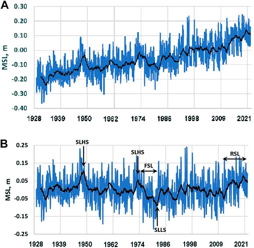
FIGURE 2. Monthly mean sea level from the NOAA Station 87202188 from 1928 to 2022. The station is located in Mayport, FL. Panel (A) shows the sea-level record including a 94-year trend of rising sea level. Panel (B) shows the sea-level record without trend, along with prominent sea-level high stands (SLHS), sea-level low stands (SLLS), periods of falling sea level (FSL), and rising sea level (RSL).

For comparison with coastal sand volume evolution at the decadal time scale, the focus in this paper is seasonal to inter-annual sea level variations during the 2006–2022 period. Figure 3 shows the water level record for this period collected at the Sebastian Inlet and verified by comparison with records from the NOAA CO-OPS Station 8721604 located at Cape Canaveral, Florida. The trend line shown in Figure 3 represents a 10-mm yr^-1 rate of RSL rise for the 2006–2022 period. This agrees with the analysis of Dangendorf et al. (2022) who reported a recent peak in RSL rise, approaching 10 mm yr⁻¹. The recent rapid rise in the sea level is also shown in Figure 2B within the longer-term trend.

FIGURE 3

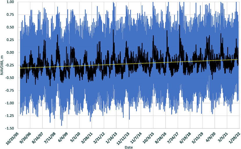
FIGURE 3. Water level record at the Sebastian Inlet collected from 2006 to 2022. The solid black line is the non-tidal sea level, and the dashed line is a 15-year sea-level rise trend of 10 mm yr^-1.

Figure 4 compares the filtered sea-level record shown in Figure 3 with the GS flow in terms of Sverdrup units of 10⁶ m³/s. The Gulf Stream flow is based on daily mean transport estimates of the Florida Current from the submarine cable voltages induced the flow. NOAA provides the daily GS flow average at https://www.aoml.noaa.gov/phod/floridacurrent/index.php. The inverse relationship between coastal ocean sea level and GS flow is clear, including annual low stands of sea level in late summer, followed by an annual high stand of sea level about 3 months later in the fall. The relation between the GS flow and coastal sea-level change is well-documented (see Ezer et al., 2013). The seasonal high rate of GS flow during the summer produces strong cross GS pressure gradients in the overall geostrophic balance that results in lower sea levels at the coast. This is followed by slowing of the GS flow and decrease in the cross-flow pressure gradient, and in response, a rapid rise of coastal sea level is observed. Along the central Florida coast, the difference between the summer low stand of sea level and fall high stand of sea level can be 70 cm or greater and includes the inter-annual variability of the annual extremes. The Florida coastal ocean sea level is strongly influenced by the interannual and decadal time scale by the dynamics of North Atlantic circulation and GS flow, as described by Ezer et al., 2013.

FIGURE 4

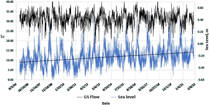
FIGURE 4. Comparison of the Gulf Stream (GS) flow and sea-level records from 2006 to 2021. The GS flow is given in sverdrup units, in which 1 Sv is 10⁶ m³/s.

The sea level during 2006–2021 shown in Figure 5 includes semi-annual and annual averages extracted from the full spectrum of water-level data shown in Figure 3. In this view, the seasonal signal is very apparent, along with shifts to both higher and lower levels within the 15-year trend to higher sea level. The trend and variability seen in sea-level records shown in Figure 3–5 are consistent with the analysis of sea level, as discussed by Dangendorf et al. (2022), Ezer et al. (2013), and other works concerned with north Atlantic circulation dynamics such as Hong et al. (2000).

FIGURE 5

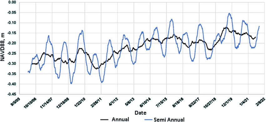
FIGURE 5. Sea-level record on the central Florida coast shown as a semi-annual and annual average over a 15-year period from 2006 to 2021. Semi-annual average emphasizes the seasonal cycle.

4 Interannual evolution of shoreface sand volume

Consideration of the influence of sea level on coastal sediment dynamics and morphological dynamics using more than projected long-term trends has been limited. However, a working knowledge of variability of coastal ocean sea level from the observational data and theoretical considerations at time scales consistent with short- to intermediate-term planning is beneficial in examining coastal response to sea-level changes at the interannual to decadal time scale. Rates of RSL rise are often applied in modeling efforts using a Bruun Rule or modified Bruun Rule approach, as described in Rosati et al. (2013). The sea-level term is usually stated as a trend based on measured records or projected sea-level rise scenarios exemplified by the recent NOAA analysis of projected rates (Sweet et al., 2017). In the present study, a topographic data set of relatively high temporal and spatial resolution is compared with the measured record of the coastal sea level at the decadal time scale under the hypothesis that the coastal sediment volume can respond to inter-annual sea-level changes of a significant magnitude.

To examine the influence of decadal scale inter-annual sea-level variations, the topographic data set shown in Figure 6 is divided into a series of nine shoreface sediment budget volume cells, as shown in Figure 7. Sediment volumes within each cell were calculated to the seaward extent of the survey data at the base level of −12.2 m relative to the NAVD88 data. Sediment volume differences were then calculated in each semi-annual survey between 2006 and 2021. Figure 8 compares annual average sea level and cumulative sand volume change in the sediment budget cells. In this example, the shoreface sediment volume varies inversely with sea-level changes with a lag period of up to 18 months. This is particularly apparent in the cells north of the Sebastian Inlet that have received minimal beach nourishment over the study period (Figure 8A). The N1 and S1 cells near the tidal inlet have a larger temporal variability in sand volume and a weaker trend of change over time. Sand volume losses over the period increased with distance both north and south of the Sebastian Inlet. The visual inverse correlation between the sea-level change and sand volume change is also stronger with distance from the tidal inlet. Sand volume losses are particularly large during a period of rising sea level from 2010 to 2015. During this 5-year period, a sea-level rise of about 16 cm occurred. Sand volume losses reversed to sand volume gains in most cells between 2015 and 2018, corresponding to a net drop in sea level about 7 cm during this period. Following the pattern, sand volumes again declined after 2018, corresponding to a rise in sea level that reached 9 cm by 2022 (Figures 8A,B). Volume changes in all sediment budget cells followed this pattern except in S1 cells immediately on the south side of the Sebastian Inlet. The volume record of the S1 cell is strongly influenced by beach fill placed by four sand bypass projects between 2007 and 2022. As explained in the following sections, sand volume exchanges through the system of inlet shoals and beach fill placement have a stronger influence on the sand volume cells adjacent to the Sebastian Inlet.

FIGURE 6

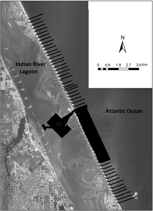
FIGURE 6. Pattern of hydrographic survey lines in the study area. A heavy pattern indicates either closely spaced lines in the back barrier areas or a multi-beam swath bathymetry survey pattern on the ocean side.

FIGURE 7

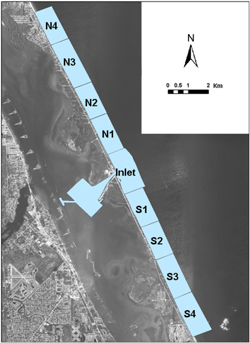
FIGURE 7. Sand volume cells in the study are within which cumulative sediment volume changes are calculated between 2006 and 2022.

FIGURE 8

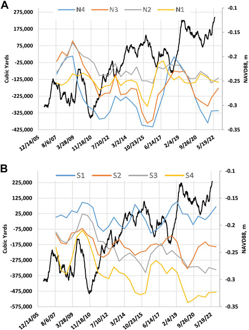
FIGURE 8. Comparison of the central Florida coast sea-level record and cumulative sand volume changes north (Panel (A))and south (Panel (B)) of the Sebastian Inlet. See Figure 7 for the cell location.

Figure 9 plots a 15-year time series of a significant wave height measured over a water depth of approximately 8.5 m approximately 1.5 km to the northeast of the Sebastian Inlet. Seasonal variability is apparent in the plot including peak wave heights in the range of 3–5 m, corresponding with the passage of tropical storms and hurricanes. Figure 10 shows one of the links between sea level and the occurrence of storms and associated storm wave. Late season hurricanes Ian and Nicole impacted the Florida coast just as sea level reached an annual high stand in late October and early November 2022, correlating with the drop in the GS flow (Figure 10). Between the annual low stand of coastal sea level in August 2022 and the annual high stand of sea level 3 months later, coastal sea level increased by 60–70 cm. Combined storm surge and storm waves at higher sea levels intensifies the overall storm impacts. This process integrated over the inter-annual time scale produces the coastal sediment volume response shown in Figure 8.

FIGURE 9

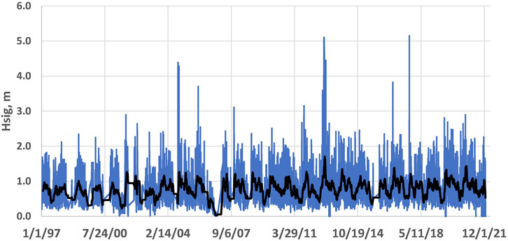
FIGURE 9. Significant wave heights in the nearshore coastal ocean of the central Florida coast recorded at a 3-h interval between 2006 and 2021.

FIGURE 10

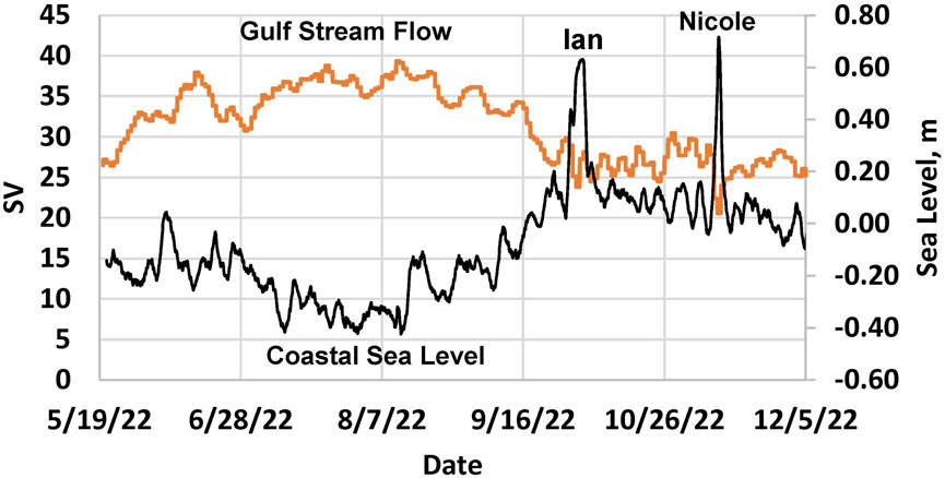
FIGURE 10. Central Florida coastal sea level compared with the GS flow, Mayport, through December 2022. Two hurricane storm surges occur during the fall 2022 high stand of coastal sea level. The GS flow is given in sverdrup units, in which 1 Sv is 10⁶ m³/s.

As established from analysis of multi-decadal sea-level oscillations by Dangendorf et al. (2022) and several other groups, sea level has been rising at higher rates since about 2000 along the southeast coast of the U.S. The sea-level record shown in Figure 8 has an overall trend of sea-level rise but includes periods of strong oscillations lasting 2–5 years. A statistical analysis of sea level versus sediment volume changes is underway but not yet complete and may require a longer record of comparison for statistically significant results. However, the visual correspondence is clear and includes lag times between sea level and sand volume peaks, and troughs of several months to more than a year. The response time of the coastal sand reservoir to changing sea level is likely to be influenced by frequency of storms and variations in wave climate. The interaction of storms and sea-level shown in Figure 10 can be thought of as the immediate cause and underlying driver of coastal change, respectively.

5 Sand budget of a transgressive coast

Analysis of sand volume and sea-level changes along the central Florida coast presented in this study provides an opportunity to interpret a sediment budget during a period of rising sea level and overall sand volume losses. There is also an opportunity to consider the influence of regional sand management schemes in the context of rapidly rising sea level. The Sebastian Inlet Management District, established in 1919, has an ongoing management plan that includes dredging of sediment from an internal sand trap at a time period of approximately 5 years and placement of the dredged material on beach to the south within about 4 km of the inlet entrance. To examine the sediment budget over the 15-year record of sea-level and sediment volume changes, the sand volume cells shown in Figure 7 were divided into upper shoreface and lower shoreface components, as shown in Figure 11. The upper shoreface sand budget cells (A cells) begin in the dune or at the vegetation line and terminate at a depth of −6 m. The seaward cells (B cells) begin at −6 m and terminate at a depth of −12.2 m. The upper shoreface sand budget cells extend to an approximately fair weather wave base in the central Florida area, whereas under storm conditions, the wave base can extend to −12 m and beyond.

FIGURE 11

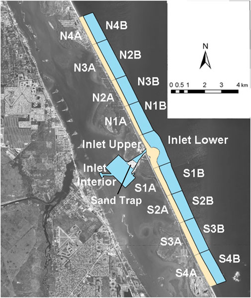
FIGURE 11. Sediment budget cells adapted from the sand volume cells. Upper shoreface budget cells labeled A extend to a depth of −6 m, whereas the lower shoreface cells extend to a depth of −12.2 m. A sediment management sand trap is shown within the inlet interior cell.

Sediment budget calculations apply conservation of mass to balance and quantify sediment sources, sinks, and sand transport pathways in a littoral cell environment, as described by Rosati (2013). The sediment budget, as applied here, demonstrates the pathways of net sediment transport at the decadal time scale and provides a view of the large-scale morphological responses of the coastal system to variable sea levels at this time scale. The sediment budget equation as expressed by Rosati (2013) is

${\displaystyle \sum }{Q}_{source}-{\displaystyle \sum }{Q}_{\mathrm{s}\mathrm{i}\mathrm{n} k}-∆V+P-R=residual.(1)$

The sources (Q_source) and sinks (Q_sink) in the sediment budget, together with net volume change within each cell (ΔV), and the amounts of material placed in (P) and removed from (R) from a cell are calculated to determine the residual volume. For a completely balanced cell, the residual would equal zero (Rosati and Kraus, 1999). Concepts and detail methodologies and recommendations for calculating coastal sediment budgets are given in Rosati (2013). The net topographic change used to calculate ΔV terms over the 15-year sand budget analysis is shown in Figure 13. Blue spectrum colors indicate erosion sand volume loss, whereas the yellow spectrum colors indicate deposition and sand volume increase. The pattern indicates that erosion on the upper and lower shoreface, and sand loss volume dominate. However, in the vicinity of the entrance to Sebastian Inlet, deposition and sand volume gain dominate. The net topographic change shown in Figure 12 is captured in terms of sediment volume change within each of the sediment budget cells shown in Figure 11

FIGURE 12

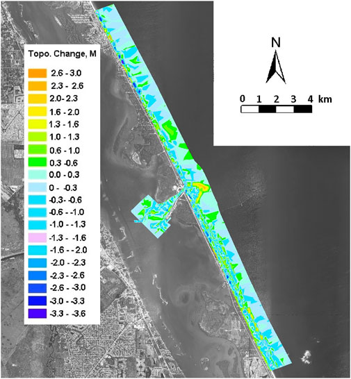
FIGURE 12. Pattern of net topographic change in the study areas between 2006 and 2021. Blue spectrum colors indicate erosion and volume loss, whereas yellow spectrum colors indicate sediment deposition and net topographic gain.

The sediment budget calculation begins with an input of 150000 m³ into cell N4 at the north end of the sediment budget series and assumes net south littoral transport. The initial input rate is based on a super-regional analysis of shoreface profile datasets collected over a 30-year period by the Florida Department of Environmental Protection (Zarillo et al., 2007). The super-regional analysis area extends from Cape Canaveral, Florida, southward for approximately 100 km. Within this larger sediment budget domain, the calculated annualized littoral transport rate at the north end of the sand budget domain surrounding the Sebastian Inlet (Figure 7) is approximately 150000 m³ yr-¹. Details of the superregional sediment budget analysis can be found in Zarillo (2007).

The calculated 15-year sediment budget is shown in Figure 13 and follows the terms in Eq. (1). The annualized volume changes (ΔV) for each cell are labeled in white along with any annualized placement (P) volume and annualized removal (R) volume. Budget cells that lost volume are shown in red, whereas cells gaining volume over the 15-year period are shown in blue.

FIGURE 13

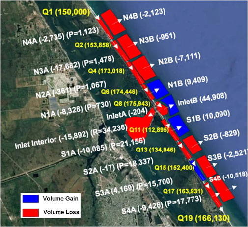
FIGURE 13. Sediment budget calculation for the 2006–2021 period based on sand volume changes calculated in the upper and lower shoreface cell and the inlet cells shown in Figure 11. Sand volume changes are annualized and given in terms of m³ yr⁻¹. Calculated longshore transport rates (Q) are also given in m³ yr⁻¹. P= placement of beach fill annualized in m³ yr⁻¹. R= removal of the sediment volume, by dredging of the sand trap in this case, also given in m³ yr⁻¹.

All ΔV, P, and R parameters have known values. In this case, the only removed (R) sand volume is from the sand trap within the interior inlet cell (see Figure 11). The annualized placement (P) values are taken from beach nourishment project records and annualized for the period of record. Beach fill placement is in the upper cells, but could be transported to the lower cells, along with spreading in the alongshore direction. Sediment exchanges between cells are shown by the white arrows. The calculated annualized longshore sediment transport rates (Q-values) based on analysis over the 15-year period are listed in yellow text in Figure 13.

The 15-year sand budget, as shown in Figure 13, is consistent with a period of sea-level rise and requires net export of sediment offshore beyond the seaward base of the lower shoreface budget cells (B cells) to balance the sediment budget. A depth of closure concept is not applied in this case since survey data indicate measurable topographic changes at depths of at least −12.2 m. In this analysis, no residual volumes were permitted, and therefore, all sediment budget cells are balanced. The annualized longshore transport rates are computed by balancing the upper shoreface sediment budget cells with alongshore annualized vectors (Figure 13). A strategy is to keep the computed longshore transport rate similar among all the upper shoreface sediment budget cells except for cells in the immediate area of the tidal inlet. The lower shoreface sediment budget cells were balanced by sending any residual sand volume offshore beyond base of the cells at −12.2 m.

Most of the calculated sediment budget is based on sand volume losses. However, relatively large annualized sand volume gains are seen in the lower shoreface cells surrounding the entrance of the Sebastian Inlet (Figure 13). These gains are balanced by sand volume losses from the adjacent upper shoreface budget cells. The vectors leading into and out of the upper shoreface Inlet A cell (Figure 13) represent capturing of sediment from littoral processes by tidal currents and wave–current interaction, and re-distribution to the lower shoreface and interior of the inlet system. In addition, this area of the sediment budget is influenced by a sediment deficit created by dredging of the sand trap (Figure 11) at approximate 5-year intervals. The reduction in the annualized longshore sediment transport rate across the inlet zone should be noted by about 60000 m³ yr-¹. Sediment transferred to the interior inlet cell and to the lower shoreface cells is known to be in the fine sand range (Zarillo et al., 2012). The large sand volume gains over the lower shoreface surrounding the inlet entrance are likely to be derived, in part, from beach fill sand dredged from the sand trap (Figure 11), which is in the fine sand range and similar in texture to the lower shoreface sediment.

5.1 Limitations to sediment budget calculations

Sediment budget calculations always have a level of uncertainty and are sensitive to assumptions about sediment sources and sinks, as well as possible errors in measured data or model data used to define the terms of a budget. These considerations are reviewed in Rosati (2005). Methods used to acquire the topographic data from which sand volume calculations are derived in this study are considered state of the art with respect to single-beam and multi-beam acoustic data collected with benchmark referenced real-time kinematic positioning (RTK). Vertical accuracy is on the order of 1 cm under the relatively calm sea states during which data are collected. Horizontal positioning is within a fraction of a meter. These accuracy levels could add errors on the order of 1% in volume calculations on the order of 50000 cubic meters. A greater source of error is interpolation between and among survey lines within a GIS software platform. In this study, where multi-beam acoustic survey methods were used, interpolation error is at a minimum. In other areas of this study, interpolated sediment volume data could significantly diverge from reality. However, the volume calculations applied in the sand budget are considered to have overall accuracy but could be of lower precision in areas of limited survey spatial resolution.

In the case of the central Florida coast, sediment budget calculations are guided by a combination of high-resolution survey data, knowledge of recent sea-level changes, and the recognition that the coastal shoreface sand reservoir is likely to be in a period of transgressive pressure exerted by several decades of rapid sea-level rise. The details of the sediment budget shown in Figure 13 could be re-interpreted for the magnitude and patterns of sediment exchanges among the budget cells, especially for cross-shore sediment exchanges. However, the overall patterns and magnitudes of sand volume movement are considered correct to a first order. The presence of a managed tidal inlet in the sand budget domain adds another layer of interpretation complexity. The deficit created by capture of sand volume in tidal inlet shoals is likely intensified by dredging of the sand trap within the interior of the inlet system. However, calculation of the sediment budget indicates that placement of this material as beach fill along with beach fill from other sources has nominally mitigated sand volume losses when sand volume changes are considered within the combined upper and lower N1 and S1 sediment budget cells. When considered separately, sand volume losses in the upper shoreface N1A and S1A cells nearly equal volume gains in their lower shoreface counterparts N1B and S1B, respectively (Figure 13)

6 Conclusion

This study demonstrates an observed relation between volume changes in the coastal shoreface sediment reservoir and large sea-level changes at the interannual to decadal time scale. Sand volume variability and overall sand volume losses along the Central Florida coast over the past 15 years can be directly linked with observed sea-level variations and the well-documented rapid sea-level rise along the southeast coast of the U.S. during this period. This opens the door to more refined predictions of coastal response at shorter time scales than the typical planning horizons of 50–100 years linked to longer-term sea-level scenarios.

There is a potential for coupling numerical modeling and machine learning methods to forecast the state of coastal morphology at the interannual to decadal time scale. To accomplish forecasting of coastal change based on rapid decadal scale sea-level oscillations, datasets like those described in this paper must be available for coastal areas threatened by ongoing rapid sea-level rise and transgression. Vulnerability to inundation and the transgression rate of coastal sedimentary environments could be determined at the interannual to decadal time scale with a good degree of accuracy.

Barriers to improved forecasting include the cost of ongoing coastal survey data, even in threatened areas, as well as limitations on understanding and forecasting the details of sea-level variability and rise at the regional spatial scale and decadal time scale. However, advances are being made in differentiating inter-annual sea-level variability from longer-term trends, as demonstrated by Dangendorf et al. (2022). Regional sterodynamic oceanographic processes have been identified that account for coastal sea-level variability like that seen along the East Coast of Florida and along the southeast U.S. in general (Ezer et al., 2013). Further understanding of the cyclicity of these processes in the realm of global climate change modeling could improve regional sea-level forecasts (Ezer and Atkinson, 2014, Hamlington et al., 2022, Karegar et al., 2016, Rahmstorf et al., 2015, Sella et al., 2007, Wdowinski et al., 2020, Zarillo et al., 2021).

Data availability statement

The datasets presented in this study can be found in online repositories. The names of the repository/repositories and accession number(s) can be found at: https://research.fit.edu/wave-data/real-time-data/.

Author contributions

The author confirms being the sole contributor of this work and has approved it for publication.

Funding

The Sebastian Inlet Management District provided funding for the data collection and analysis applied in this study.

Conflict of interest

The author declares that the research was conducted in the absence of any commercial or financial relationships that could be construed as a potential conflict of interest.

Publisher’s note

All claims expressed in this article are solely those of the authors and do not necessarily represent those of their affiliated organizations, or those of the publisher, the editors, and the reviewers. Any product that may be evaluated in this article, or claim that may be made by its manufacturer, is not guaranteed or endorsed by the publisher.

References

Church, J. A., and White, N. J. (2011). Sea-level rise from the late 19th to the early 21st century. Surv. Geophys. 32 (4-5), 585–602. doi:10.1007/s10712-011-9119-1

CrossRef Full Text | Google Scholar

Dangendorf, S., Hendricks, N., Sun, Q., Klinck, J., and Ezer, T., Acceleration of US southeast and Gulf coast sea-level rise amplified by internal climate variability, Nature Communications, 14, 1, 1935, 2023.

PubMed Abstract | CrossRef Full Text | Google Scholar

Ezer, T., and Atkinson, L. P. (2014). Accelerated flooding along the U.S. East coast: On the impact of seasea-level rise, tides, storms, the Gulf Stream, and the North Atlantic oscillations. Earth’s Future 2, 362–382. doi:10.1002/2014EF000252

CrossRef Full Text | Google Scholar

Ezer, T. (2013). Sea level rise, spatially uneven and temporally unsteady: Why the US East Coast, the global tide gauge record, and the global altimeter data show different trends. Geophys. Res. 40 (20), 5439–5444. doi:10.1002/2013gl057952

CrossRef Full Text | Google Scholar

Hamlington, B. D., Chambers, D. P., Frederikse, D., Soenke, T., Fournier, S., Buzzanga1, B., Steven Nerem, R., et al. (2022). Observation-based trajectory of future sea level for the coastal United States tracks near high-end model projections. Commun. Earth Environ. 3, 230. doi:10.1038/s43247-022-00537-z

CrossRef Full Text | Google Scholar

Karegar, M. A., Dixon, T. H., and Engelhart, S. E. (2016). Subsidence along the atlantic coast of North America: Insights from GPS and late holocene relative sea level data. Geophys. Res. Lett. 43, 3126–3133. doi:10.1002/2016gl068015

CrossRef Full Text | Google Scholar

Rahmstorf, S., Box, J. E., Feulner, G., Mann, M. E., Robinson, A., Rutherford, S., et al. (2015). Exceptional twentieth-century slowdown in Atlantic Ocean overturning circulation. Nat. Clim. Change 5, 475–480. doi:10.1038/nclimate2554

CrossRef Full Text | Google Scholar

Rosati, J. D. (2005). Concepts in sediment budgets. J. Coast. Res. 21 (2), 307–322. doi:10.2112/02-475a.1

CrossRef Full Text | Google Scholar

Rosati, J. D., Dean, R. G., and Walton, T. L. (2013). The modified Bruun Rule extended for landward transport. Mar. Geol. 340, 71–81. doi:10.1016/j.margeo.2013.04.018

CrossRef Full Text | Google Scholar

Rosati, J. D., and Kraus, N. C. (1999). Sediment budget analysis system, Coastal and Hydraulics Laboratory, Kitty Hawk, CA, USA.

Google Scholar

Sella, G. F., Stein, S., Dixon, T. H., Craymer, M., James, T. S., Mazzotti, S., et al. (2007). Observation of glacial isostatic adjustment in “stable” North America with GPS. Geophys. Res. Lett. 34 (1–6), L02306. doi:10.1029/2006gl027081

CrossRef Full Text | Google Scholar

Sweet, W., Kopp, R., Weaver, C., Obeysekera, J., Horton, R., Thieler, E., et al. (2017). Global and regional Sea Level rise scenarios for the United States, https://ntrs.nasa.gov/citations/20180001857 Silver Spring MD.

Google Scholar

Wdowinski, S., Oliver-Cabrera, T., and Fiaschi, S. (2020). Land subsidence contribution to coastal flooding hazard in southeast Florida. Proc. IAHS 382, 207–211. doi:10.5194/piahs-382-207-2020

CrossRef Full Text | Google Scholar

Zarillo, G. A., Brehin, F., Erickson, L., Cote, C., and Hearin, J. (2012). State of sebastian inlet annual report; an assessment of inlet morphologic processes, shoreline changes, sediment budget, and beach fill performance, https://www.sitd.us/files/faa429990/State+of+the+Inlet+2012.pdf

Google Scholar

Zarillo, G. A., RamosS Habib, A., and Rosario-Llantín, J. (2021). State of sebastian inlet annual report; an assessment of inlet morphologic processes, shoreline changes, sediment budget, and beach fill performance, https://www.sitd.us/files/f87e7dc80/State+of+Sebastian+Inlet+2020+final.pdf.

Google Scholar

Zarillo, G. A., Watts, I. M., Erickson, L., Brehin, F., Hall, K. L., and Chauhan, S. N., State of sebastian inlet report 2014: An assessment of inlet morphologic processes, shoreline changes, sediment budget and beach fill performance, Florida Institute of Technology, Melbourne, FL, USA.