Varying performance of eight evapotranspiration products with aridity and vegetation greenness across the globe

The wide application of the evapotranspiration (ET) products has deepened our understanding of the water, energy and carbon cycles, driving increased interest in regional and global assessments of their performance. However, evaluating ET products at a global scale with varying levels of dryness and vegetation greenness poses challenges due to a relative lack of reference data and potential water imbalance. Here, we evaluated the performance of eight state-of-the-art ET products derived from remote sensing, Land Surface Models, and machine learning methods. Specifically, we assessed their ability to capture ET magnitude, variability, and trend, using 1,381 global watershed water balance ET as a baseline. Furthermore, we created aridity and vegetation categories to investigate performance differences among products under varying environmental conditions. Our results demonstrate that the spatial and temporal performances of the ET products were strongly affected by aridity and vegetation greenness. The poorer performances, such as underestimation of interannual variability and misjudged trend, tend to occur in abundant humidity and vegetation. Our findings emphasize the significance of considering aridity and vegetation greenness into ET product generation, especially in the context of ongoing global warming and greening. Which hopefully will contribute to the directional optimizations and effective applications of ET simulations.

1 Introduction

Terrestrial evapotranspiration (ET), as a pivotal element of such land-atmosphere interaction processes as what happens to water, carbon, and energy cycle, is constituted of soil evaporation, vegetation transpiration and water surface evaporation (Gao et al., 2016; Tramontana et al., 2016; Zhang et al., 2016; Liu et al., 2021). On the land surface, 60% of precipitation (Pre) is returned to the atmosphere through ET, consuming half of the solar energy reaching at the surface (Pan et al., 2020). Consequently, ET draws significant interest from hydrology to climate disciplines. Researchers aim to understand the allocation of energy and water at the land and its feedbacks (Zhang et al., 2017), identify dominant control factors of ET variation across regions (She et al., 2017; Zhang et al., 2021), and investigate the impact of ET on the hydrological cycle under climate change (Gu et al., 2020; Weerasinghe et al., 2020). Hence, accurate estimation of ET is crucial for various scientific communities such as hydrology, ecology, climatology, and agriculture.

There is no denying that existing ET products have considerable potential to facilitate the estimation of hydrological and energetic components and their inherent hydroclimatic variability. For instance, global ET estimates at arbitrary spatial and temporal scales can be compiled by the conventional flux formula (or Land Surface Model (LSM)) and the remote sensing observations about surface temperature, soil moisture and vegetation cover ratio (Wang et al., 2016; Miao and Wang, 2020). Recently, the boom in machine learning methods has also facilitated the acquisition of global ET datasets (Jimenez et al., 2011; Alemohammad et al., 2017; Jung et al., 2017), such as model tree, random forest, or artificial neural networks combining observed flux data as inputs. However, these products simultaneously involve some uncertainties derived from the model structural flaws, input-datasets errors (e.g., meteorological forcing, land surface, and parameters related to vegetation), model-parameter errors and scale-scaling issues (Badgley et al., 2015; Michel et al., 2016; Miralles et al., 2016).

However, the existing terrestrial ET products widely vary in performance and even oppose long-term trends, indicating the non-negligible uncertainties. For instance, it has been reported that while potential evapotranspiration (PET) trends have declined over the last 50 years, ET has shown an increasing trend according to the evapotranspiration paradox (Mao et al., 2015; Zhang et al., 2015; Zeng et al., 2018). However, Jung et al. (2010) added that the increase in global terrestrial ET has ceased or even reversed from 1998 to 2008. Therefore, a comprehensive evaluation of ET products is a prerequisite for model optimizations and global climate-change research, especially, on a regional scale.

ET measurements from the Eddy Current Covariance (EC) site have become typical reference data to validate ET products at the point scale. Nevertheless, EC systems generally suffer from energy imbalance, which resulting in ET measurement errors. And the mismatch in spatial scale between EC observations and ET estimates (points and grid cells) is another limitation. Furthermore, EC sites sparsely spread over spaces, which challenges the evaluation of ET products on a regional scale (Pan et al., 2020; Xie et al., 2022). An alternative approach is terrestrial water balance method, i.e., ET calculated from the terrestrial water balance (observed Pre minus the sum of runoff (Q) and total water storage change (TWSC)) is applied as the truth value to validate ET products at the basin scale (Liu et al., 2016). Over the last 2 decades, considerable attention has focused on the regional scale (US, African, and Qinghai-Tibetan Plateau), while less on the global scale. For example, Vinukollu et al. (2011) conducted a global evaluation on the ET estimates derived from three process-based models (Surface Energy Balance System (Su, 2002), Penman–Monteith–Mu algorithm (Penman, 1948; Mu et al., 2007), and Priestly–Taylor–Fisher of Jet Propulsion Laboratory algorithm (Priestley and Taylor, 1972; Fisher et al., 2008) based on 26 basins worldwide, and suggested a root mean squared difference (RMSD) of 118–194 mm/yr and a deviation of −132 to 53 mm/yr between the water balance ET and the estimated annual ET.

However, the total water storage change (TWSC) at the annual scale has often been disregarded in previous studies (Pre directly minus Q), yet the water budget is unbalanced due to human abstraction, glacial snowmelt, and other activities affecting water storage (Liu et al., 2016; Zhong et al., 2020). For example, Zeng et al. (2012) found that the TWSC cannot be ignored in estimating ET at an annual scale, especially in regions with relatively low ET values. As a result, the annual reference ET must take into account TWSC. Although the Gravity Recovery and Climate Experiment (GRACE) satellite launched in 2002 offers a promising future to the TWSC, the limited GRACE satellite data right now makes it problematic to assess ET products with long-time data, especially the pre-2002 data, and subsequently difficult to explore ET trends. Recently, the reconstruction of GRACE facilitates the evaluation on long-time series of ET products. More importantly, the deficiencies exist in the simultaneous evaluation of ET products at the global scale with various levels of dryness and vegetation greenness. The ET variation in different regions is closely related to local conditions: ET is limited by water in dry conditions and by energy in wet conditions; ET is higher in highly-vegetated areas and lower in sparsely-vegetated areas. We postulate that these conditions may affect the performance of ET products. For example, Majozi et al. (2017) assessed the accuracy and precision of four ET products in two South African ecoregions and showed that no one ET product performed best in both zones; Ershadi et al. (2014) found that the performance of European and North American ET models varied among zones and the models with relatively high accuracy differed across zones; Kim et al. (2012) concluded that the Moderate Resolution Imaging Spectrometer (MODIS) MOD16 ET for Asian woodland cover was more accurate than for other biomes. Consequently, there is a need to fully understand the simulation capacity of ET products under heterogeneous conditions (areas with different levels of aridity and vegetation greenness), which will be favorable to developing strategies for adapting to the climate change.

Here, the current study is not to compare the various models, but to investigate how the performances of eight global ET products vary with water and energy conditions or vegetation greenness over 1981–2010. In doing so, the globally distributed 1,381 basins were taken into consideration and segmented according to their aridity and vegetation conditions. Then, we illustrated differences in the performance of the products changing with aridity and vegetation based on the terrestrial water balance ET. The model performance of the ET product was evaluated using newly popular metric–Kling-Gupta efficiency (KGE), considering the magnitude, variability of the ET and its coefficient to the product. Additionally, the 1981–2010 period was selected, for the knowledge about this period is relatively lacking and the reconstructed the total water storage anomaly (TWSA) products are reliable before 2002. Finally, we discussed the potential reasons for our results.

2 Datasets and methods

2.1 Datasets

2.1.1 Runoff (Q) datasets

To comprehensively assess the ET products, the daily Q observed at 31,133 hydrological stations across the globe were collected from 11 databases, as listed in Table 1 (Holmes et al., 2013; Arsenault et al., 2016; Awange et al., 2019; Arsenault et al., 2020; Chagas et al., 2020; Coxon et al., 2020; Almagro et al., 2021; Fowler et al., 2021; Klingler et al., 2021).

TABLE 1

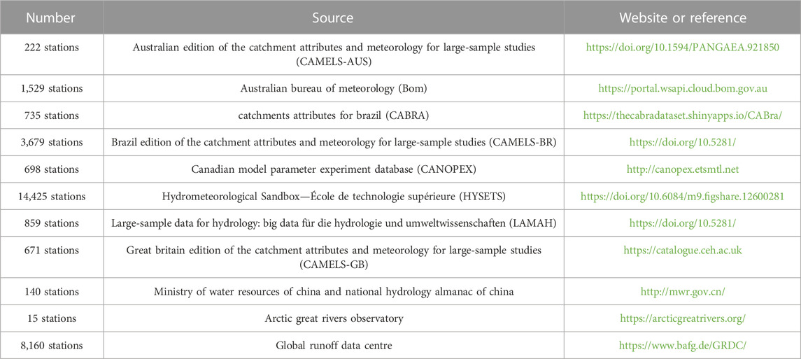
TABLE 1. Summary of Q observation sources for 11 databases of Q observation sources.

Considering that the Q dataset is derived from different sources; several criteria were implemented to control the dataset quality with reference to some well–established data processing methods (Beck et al., 2015). The details related to the criteria used in this study are as follows:

1 The final database retains a hydrological station only once, based on the latitude and longitude information of hydrological station;

2 If a station has missing data for more than 15% per day from 1981 to 2010, the station was removed;

3 The basin area controlled by the hydrological station must be able to cover two or more 0.5° grids.

Finally, 1,381 stations met these criteria. The global distribution of 1,381 hydrological stations is shown in Figure 1.

FIGURE 1

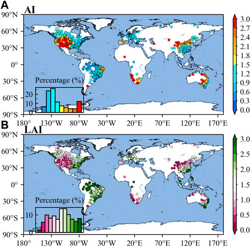
FIGURE 1. Spatial patterns of AI and LAI (A, B) of global 1,381 basins from 1981–2010. The histograms in (A, B) present AI and LAI at different levels corresponding to the color bars.

2.1.2 Precipitation and GRACE datasets

To reduce the uncertainties in precipitation data, we selected three global gridded precipitation datasets (GPCC, CPC-Unified, and CRU TS4.05) at 0.5° resolution based on precipitation gauges. GPCC precipitation dataset, was selected, for it is widely considered as the precipitation reference dataset (Becker et al., 2013). More importantly, CPC-Unified gauge-based analysis of global daily precipitation at 0.5° resolution (1979-present) was interpolated from the QC station reports, which incorporates the effects of topography (Chen et al., 2008).

Total water storage anomalies (TWSA), monitored by NASA’s GRACE satellites via satellite gravimetry, are currently used for retrieving the exclusive data of TWSC in hydrological and climatic applications (Landerer and Swenson, 2012; Long et al., 2014; Jing et al., 2020a). Notably, the GRACE TWSA observation data only covers the period 2002–2017 (Jing et al., 2020b). Consequently, the two constructed TWSA datasets (i.e., GRACE-REC and GRID-CSR-GRACE-REC) were chosen, covering the data from 1981–2010 at a spatial resolution of 0.5°. GRACE-REC datasets were generated, using a statistical model trained with GRACE observations, consisting of six reconstructed TWSA datasets derived from two different GRACE observation products and three different meteorological forcing datasets (Humphrey and Gudmundsson, 2019). As for GRID-CSR-GRACE-REC, Li et al. (2021) reconstructed the GRACE observations by developing a methodological framework to compare three methods, including the multiple linear regression (MLR), autoregressive exogenous (ARX) approaches, and artificial neural network (ANN), using as inputs Pre, sea and land surface temperature, surface and subsurface runoff, soil moisture, evaporation, and several climate indices. Please note that the Pre- TWSC for each basin was derived from the arithmetic mean value of six datasets-combination: GPCC minus GRACE-REC, CPC-Unified minus GRACE-REC, CRU TS4.05 minus GRACE-REC, GPCC minus GRID-CSR-GRACE-REC, CPC-Unified minus GRID-CSR-GRACE-REC, and CRU TS4.05 minus GRID-CSR-GRACE-REC. The basic information of the Pre and TWSA products is shown in Table 2.

TABLE 2

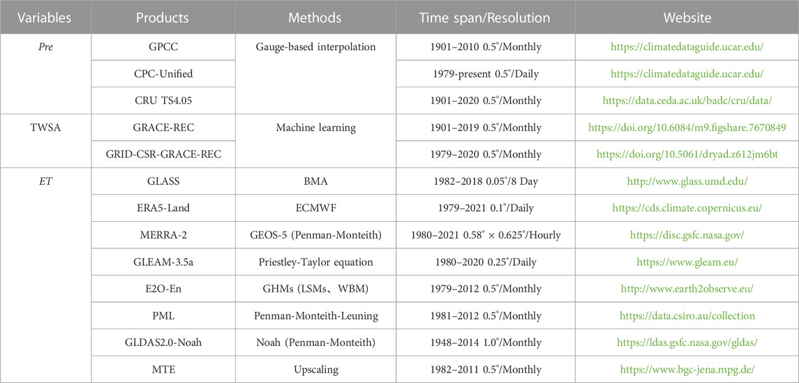
TABLE 2. Hydrological-component information of used products.

2.1.3 ET products

Eight ET products using different methods were collected in this study: one remote sensing product (GLASS), two reanalysis products (ERA5-Land and MERRA-2), four LSM-based products (GLEAM-3.5a, E2O-En, PML and GLDAS2.0-Noah), and one machine learning-based product (MTE). The basic information of the ET products is shown in Table 2.

To estimate terrestrial ET, Global LAnd Surface Satellite (GLASS) ET products used the Bayesian model averaging (BMA) method to ensemble five process-based ET algorithms (Yao et al., 2014; Xie et al., 2022), i.e., MODIS ET product algorithm (Penman, 1948; Mu et al., 2007; Mu et al., 2011), revised remote-sensing-based Penman-Monteith ET algorithm (Yuan et al., 2010), Priestly–Taylor–Fisher of Jet Propulsion Laboratory ET algorithm (Fisher et al., 2008), modified Satellite-Based Priestley-Taylor ET algorithm (Yao et al., 2013), and semi–empirical Penman ET algorithm of the University of Maryland (Wang et al., 2010). It outperforms the five algorithms by using ground-based data of 2000–2009 collected from 240 EC gauges worldwide on all continents except for Antarctica. The ensemble algorithms, integrating multiple algorithms to generate the product, reduces the uncertainties of a single algorithm and ensures the accuracy of the product. The dataset used in this study is the product with the longest time series and the finest grid, spanning from 1982 to 2018 at a grid of 0.05°.

ERA5-Land (Muñoz-Sabater et al., 2021), an enhanced global dataset for the land component of the fifth generation of European ReAnalysis (ERA5), was published by the European Centre for Medium-Range Weather Forecasts (ECMWF) in 2021. The core of ERA5-Land is the ECMWF surface model: the Carbon Hydrology-Tiled ECMWF Scheme for Surface Exchanges over Land (CHTESSEL). Four meteorological state fields (i.e., temperature, humidity, wind speed, and pressure at the surface) are available in the ERA5, from the lowest level of the model (level 137), which is 10 m above the surface. Surface fluxes involve downward shortwave, longwave radiation and total liquid, and solid precipitation. Compared with latent heat data from 65 EC gauges worldwide, ERA5-Land ET performs better than previous versions such as ERA5 and ERA-Interim (Albergel et al., 2018), benefiting from the enhancements on the ECMWF surface model. The dataset used in this study spans the period from 1979 to 2021 and has a grid of 0.1°.

The second Modern Era Retrospective-Analysis for Research and Applications (MERRA-2) reanalysis (Rodell et al., 2011), a widely used atmospheric reanalysis dataset, is provided by Global Modeling and Assimilation Office (GMAO) in NASA. It is produced by the upgraded Goddard Earth Observing System model Version 5 (GEOS-5), along with its associated data assimilation system (DAS) Version 5.12.4, which replaced the original MERRA and MERRA-Land reanalysis. MERRA-2 alleviates some of the deficiencies of the MERRA and MERRA-Land product, such as certain biases and imbalances in the water cycle as well as the false trends and jumps in precipitation associated with changes in the observing system. The dataset used in this study spans from 1980 to 2021 and has a grid of 0.58° × 0.625°.

The Global Land Evaporation Amsterdam Model (GLEAM), a set of algorithms, including a potential evaporation module, stress module, and rainfall interception module, dedicates to estimating the terrestrial evaporation and root-zone soil moisture from the satellite data, which consists of soil evaporation, canopy transpiration, interception loss, snow sublimation, and open-water evaporation (Martens et al., 2017). Among these modules, the potential evaporation module uses the Priestley–Taylor equation, and the stress module is represented by the semi-empirical relationship between vegetation optical depth and root-zone soil moisture. A vital feature of this product is that the Gash analytical model is used to estimate interception loss.

To develop the global water reanalysis on the multi-scale water resource assessment and related research projects, the EartH2Observe (E2O) project also used the reanalysis-based forcing data to drive ten models: five global hydrological models (GHMs), four Land Surface Models (LSMs) with extended hydrological scenarios, and one simple water balance model (WBM) (Schellekens et al., 2017). The forcing dataset is an adjustment of the ERA reanalysis dataset combining the terrestrial meteorological element observations and Climate Research Unit (CRU) datasets. The E2O-En product has proven to be an accurate reanalysis data and been widely used for the multi-scale water resource applications (Schellekens et al., 2017). The generated data from ten models were arithmetically averaged to alleviate the potential errors and uncertainties of the individual model.

The GLDAS is a global assimilation and modeling system developed jointly by NASA, Goddard Space Flight Center (GSFC), and NOAA (Rodell et al., 2004; Rodell et al., 2011). The system provides the near real-time land-surface information from ground and satellite observations, by driving four LSMs. Here, the ET product derived from GLDAS2.0-Noah is adopted in our study.

The Model Tree Ensemble (MTE) product, a data-driven estimate (Jung et al., 2009), was compiled using a global monitoring network (the database of the FLUXNET), the meteorological and remote-sensing observations, and a machine-learning algorithm. Its forcing data include a harmonized the Fraction of Absorbed Photosynthetically Active Radiation (FAPAR) product from three sensors (AVHRR (Tucker et al., 2005), SeaWiFS (Gobron et al., 2006), MERIS (Gobron et al., 2008), a remote-sensing-based global land-use, and products of climate variables based on observations. However, the lack of measurements makes it impossible to calculate ET in cold and dry deserts; this may result in a slight underestimation of global ET.

2.1.4 AI and LAI data

Another monthly Pre and potential ET dataset (1901–2020) was chosen from CRU TS4.05, to calculate the aridity index (AI): the ratio of Pre and potential ET. GLASS LAI product was compiled by AVHRR from 1981–2000 and by MODIS from 2001 to 2018 (Xiao et al., 2013). To generate continuous and smooth data, GLASS LAI used a temporal-spatial filtering algorithm to remove cloud contamination from the reflectance data. The vital component of this product is the algorithm to train a general regression neural networks (GRNNs), using fused LAI from MODIS and CYCLOPES products and reprocessed MODIS reflectance for each vegetation type on observation sites (Xu et al., 2018). The dataset spans the period from 1981 to 2018 and has a grid of 0.05°. Please note that all gridded datasets were aggregated to an annual temporal resolution and a spatial resolution of 0.5°. The spatial patterns of AI and LAI of global 1,381 basins are shown in Figure 1.

2.2 Methods

2.2.1 Water balance ET

Eight ET products were assessed, using water balance equations. The water-balance- based ET is often considered a reference for validating ET products on the annual scale. ET can be calculated based on precipitation (Pre), runoff (Q) and total water storage change (TWSC) in the basin, using the following equation:

$\mathbf{w}\mathbf{a}\mathbf{t}\mathbf{e}\mathbf{r}\mathbf{b}\mathbf{a}\mathbf{l}\mathbf{a}\mathbf{n}\mathbf{c}\mathbf{e}\mathit{E}\mathit{T}=\mathit{P}\mathit{r}\mathit{e}-\mathit{Q}-\mathbf{T}\mathbf{W}\mathbf{S}\mathbf{C}(1)$

Due to high correlations with static gravity fields, GRACE does not provide the estimates of total continental water content. In this aspect, TWSA is defined as the residual water content at a given time, which is relative to the water content at a reference epoch. The reference storage corresponds to the average water storage during the early phases of the GRACE mission (Han et al., 2005; Yang et al., 2020). Hence, yearly TWSC is the difference between the December anomaly observation of the current year and that of the previous year, i.e., the yearly TWSC equation is as follows:

${\mathbf{T}\mathbf{W}\mathbf{S}\mathbf{C}}_{\mathit{i}}={\mathbf{T}\mathbf{W}\mathbf{S}\mathbf{A}}_{\mathit{i},\mathbf{D}\mathbf{e}\mathbf{c}}-{\mathbf{T}\mathbf{W}\mathbf{S}\mathbf{A}}_{\mathit{i}-\mathbf{1},\mathbf{D}\mathbf{e}\mathbf{c}}(2)$

where i and Dec denote the year (ranging from 1981–2010) and the December, respectively.

2.2.2 Evaluation metrics

Kling-Gupta efficiency (KGE) and its three components are used to further evaluate the eight ET products (Kling et al., 2012). KGE is an objective performance metric, which comprehensively combines the components of the key performance statistics (correlation, bias and variability). The KGE formulation is defined as follows:

$\mathit{K}\mathit{G}\mathit{E}=\mathbf{1}–\sqrt{{\left(\mathit{R}-\mathbf{1}\right)}^{\mathbf{2}}+{\left(\mathit{\beta }-\mathbf{1}\right)}^{\mathbf{2}}+{\left(\mathit{\gamma }-\mathbf{1}\right)}^{\mathbf{2}}}(3)$

where $R$ is Pearson’s correlation coefficient, $\beta$ is the bias (the ratio of the estimates and observation means), $\gamma$ is the variability [the ratio of the coefficients of variation (CV)].

$\mathit{\beta }=\frac{{\mathit{\mu }}_{\mathit{e}}}{{\mathit{\mu }}_{\mathit{o}}}(4)$

$\mathit{\gamma }=\frac{{{\mathit{\sigma }}_{\mathit{e}}/\mathit{\mu }}_{\mathit{e}}}{{{\mathit{\sigma }}_{\mathit{o}}/\mathit{\mu }}_{\mathit{o}}}(5)$

where $\mu$ and $\sigma$ denote the mean and the standard deviation, respectively; e and o denote the estimate and the observation. Note that the ranges of KGE, R, $\beta$ and $\gamma$ with the optimum value of 1.0 are −∞–1.0, −1.0–1.0, −∞–+∞ and −∞–+∞, respectively. A comprehensive diagnosis was carried out on the performance of ET products in capturing ET characteristics at the temporal and spatial scale. Please note that the hit of ET trend directions for each product was also evaluated, using the ratio of truly captured ET trend directions including positive and negative trends. For example, TPR (FPR, TNR, FNR) denotes the ratio between the number of basins that the ET products truly (falsely, truly, falsely) identify the observed positive (positive, negative, negative) ET trend as positive (negative, negative, positive) ET trend and the number of all basins. The sum of TPR, FPR, TNP, and FNR is equal to 100%. To systematically assess the spatial and temporal capture performance of the ET products, we assessed both the spatial dynamic of ET climatological value, temporal variability and trends, and the temporal dynamic of ET for each basin.

2.2.3 Aridity and vegetation categories

If global basins are diagnosed in overall terms, the information about the performance of ET products under given conditions will be lost. Meanwhile, it is important to examine how ET products vary with water and energy conditions or vegetation greenness, since the ET process is affected by the complex mechanisms of energy, water cycle and vegetation and the strong variability in both space and time. Therefore, the aridity and vegetation categories were created without considering their changes during the evaluation period, for the sake of simplicity. Specifically, the aridity index (AI) is characterized by the long -term climatic aridity condition of a region, for example, the higher AI value indicates the drier condition. The threshold of multiyear-average AI was set at 1.5, based on the conventional definition, i.e., basins with AI>1.5 are classified as the dry basins and those with AI≤1.5 are classified as the wet basins (Liu et al., 2016). As for vegetation, the LAI is widely applied as the proxy of vegetation greenness, with high values suggesting high greenness. Based on the LAI value for each basin at the evaluation period, the evaluation metrics were re-classified in three categories, i.e., LAI<1, 1 ≤ LAI<2 and LAI≥2, which were defined as the LAI-I, LAI-II, and LAI-III, respectively (Jimenez et al., 2011; McCabe et al., 2016), with regard to the intensity of greenness (from brown to green).

3 Results

3.1 Overall assessment of ET products

Figure 2A shows the spatial pattern of the mean annual value of ET during 1981–2010. The high values (>1,000 mm) mainly existed in the Brazilian coast, the GulfofMexico and Atlantic coasts in America, the African coast, and the Oceania East coast. Specifically, the ET decreased from east (west) to west (east) across the North (South) America, and from southeast to northwest across China. By contrast, the spatial variability of ET CV was not line with the ET value: the high ET occurred in the Amazonian Plain and Brazilian plateau, whereas high ET CV occurred in South China (Figure 2B). Additionally, the ET tended to increase in the Eurasia and Brazilian plateau, while decreasing in the Amazonian Plain (Figure 2C). Overall, about 20% of basins showed the significant trends, and the significant increases were mainly in the Northwest China, Europe, and the midwest U.S, while the significant decreases were mainly in the Congo Basin and Amazonian Plain) (Figure 2D). In conclusion, ET regarding magnitude, temporal variability and trend showed the high spatio-temporal heterogeneity.

FIGURE 2

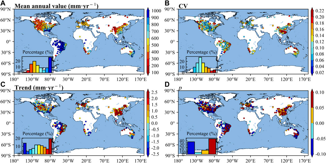
FIGURE 2. Spatial patterns of water balance ET at global 1,381 basins during 1981–2010. Small letters (A–D) represent the mean annual value, CV, trend, and significance level (p < 0.05) of trend, respectively. The histograms in (A–D) present the ET of different levels corresponding to the color bars.

All ET products could reproduce the spatial distribution for climatological values of ET with high spatial R values ≥ 0.90 (Table 3). Among these products, the PML performed slightly better than the other products with the highest and R value of 0.96, though not with optimal $\beta$ and $\gamma$. The $\beta$ values for most ET products were consistently around the optimal value of 1.0, except for GLASS (1.27 for $\beta$) and MERRA-2 (1.22 for $\beta$), suggesting that the magnitudes of climatological values were well captured by most ET products. However, the spatial variabilities of ET tended to be underestimated by most ET products with 0.7< $\gamma$ <1.0, especially for ERA5-Land with a $\gamma$ of 0.74. The values of R, $\beta$ and $\gamma$ for capturing the ET by the products converged to the optimum value of 1.0, resulting in KGE values of integrative performances that outweighed 0.71. Notably, the model-based products had higher overall performance (KGE ≥ 0.81) in reproducing the climatological ET, compared to the reanalysis products (0.71 ≤ KGE < 0.81). Regarding the temporal variability, all ET products generally underestimated the CV (0.34≤ $\beta$ ≤0.89), but evidently overestimated its spatial variability (1.21≤ $\gamma$ ≤2.39). Moreover, the spatial distribution of ET CV were poorly captured be most ET products, with GLEAM-3.5a having the maximum R value of 0.25 among the eight ET products. Overall, the KGE values were mostly negative, ranging from −0.80 (MTE) to 0.04 (MERRA-2), indicating that most ET products had limited KGE-based ability to simulate ET temporal variability. In the view of the ET trend, the directions (i.e., upward and downward) could be hit by most products, with 59.29% for PML ≤ TPR + TNR≤65.66% for MERRA-2. However, the FPR, near to and even larger than the TNR, suggested that the negative trends would be misidentified as positive trends, especially for GLASS (39.68% versus 3.04%). The R values ranged from 0.09 (MTE) to 0.36 (MERRA-2) indicating that GLASS and MERRA-2 with values above 0.30 could capture the ET trends in space. Except for reanalysis products underestimating the ET trend, all others overestimated the ET trend, with $\beta$ larger than 1.0. By contrast, all products underestimated the spatial variability of the ET trend, with −0.19 (MERRA-2)≤ $\gamma$ ≤0.18 (GLEAM-3.5a). All KGE values were negative, indicating that these poor overall performance of these ET products in capturing the ET trend.

TABLE 3

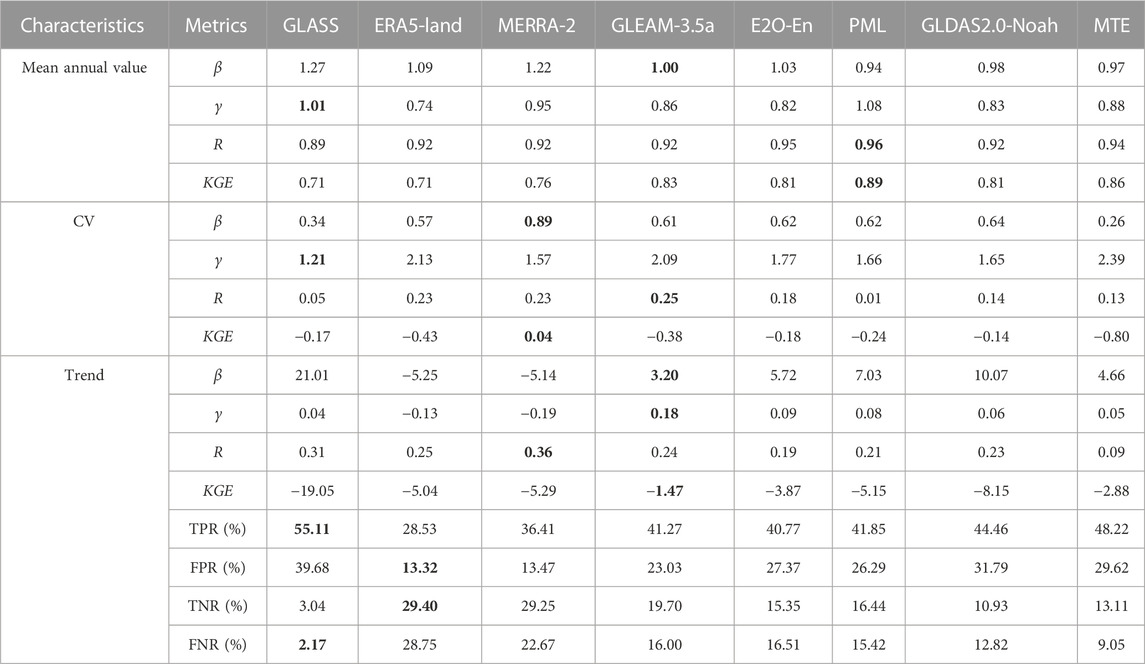
TABLE 3. The evaluation results of eight ET products against water balance ET during 1981–2010 from global 1,381 basins. Bold numbers in the table represent the optimal results corresponding to each metric.

Figure 3 shows the metrics of $\beta$, $\gamma$, R, and KGE for 1,381 basins. The majority of ET products overestimated ET at more than 50% of basins, especially GLASS and MERRA-2 which overestimated ET at above 92% of basins (Figure 3A). However, PML, GLDAS2.0-Noah and MTE underestimated the ET at more than 50% of basins. Spatially, the $\beta$ values displayed evident spatial differences, with most of ET products greatly overestimated the ET in China, Europe, and North America. Considering the metric of $\gamma$ (Figure 3B), all ET products tended to underestimate the ET temporal variabilities at over 70% of basins. When $\gamma$ <0.2, ET products, especially MTE and GLASS, underestimated the ET temporal variabilities at around 30% of basins worldwide. Additionally, the overestimates of ET temporal variabilities tended to be at American Midwest. About the spatial patterns of $\beta$ and $\gamma$, it is worth noting that the higher ET magnitude estimates were accompanied by lower ET variability estimates, since the ratio of basins having $\beta$ >1.0 outweighed the ratio of basins having $\gamma$ <1.0 for most ET products except PML, GLDAS2.0-Noah, and MTE (Figures 3A,B). Regarding temporal fluctuation (Figure 3C), positive R values were observed for 59.30% (MERRA-2) to 84.50% (ERA5-Land) of basins, especially MERRA-2 with R > 0.6 at nearly 20% of basins, indicating that ET products had a broad R-based ability to simulate ET temporal fluctuation. High R values (around 0.8) mainly appeared in the Midwest United States, South Africa, Western Australia. However, the average R values for all ET products were slightly low, ranging from 0.06 for GLDAS2.0-Noah–0.24 for ERA5-Land. Based on KGE (Figure 3D), negative KGE values were found in 47.65% (E2O-En) to 71.76% (MTE) of basins, with general negative basin-averaged KGE values (−0.14 (GLASS) to 0.03 (E2O-En)), indicating that all ET products had the limited overall performance for temporal scale. Relatively, the KGE > 0.2 mainly existed at Australia and Midwest America.

FIGURE 3

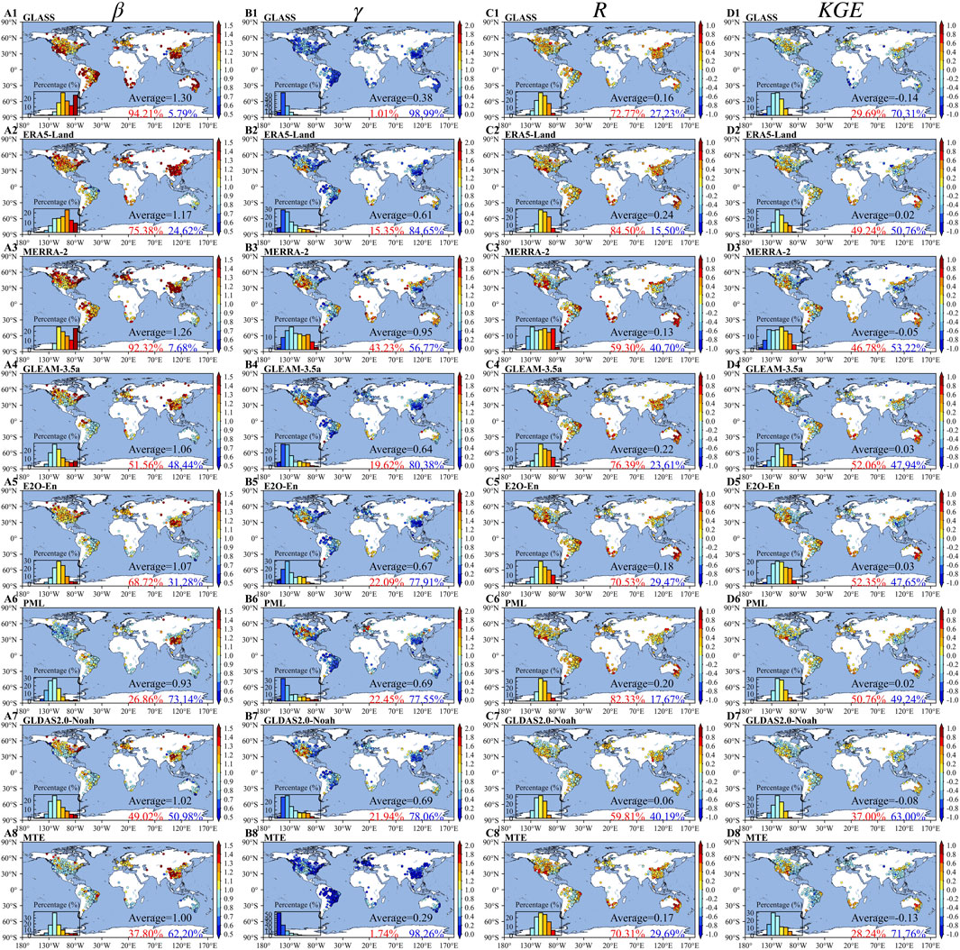
FIGURE 3. Spatial patterns of validation metrics at global 1,381 basins. The histograms in (A–D) present the values of KGE and its components R, $\beta$ and $\gamma$ at different levels corresponding to the color bars.

3.2 Validation by aridity regimes

In terms of the climatological values of ET under dry and wet conditions (Figure 4), except GLASS under all conditions and MERRA-2 under wet condition, the ET products could reproduce the magnitudes of ET with 0.86 for PML≤ $\beta$ ≤1.17 for ERA5-Land under dry condition and with 0.96 for MTE≤ $\beta$ ≤1.07 for ERA5-Land under wet condition, which was consistent with the results presented in Section 3.1 (Table 3). In particular, most of the ET products underestimated the water balance ET above 1,200 mm (Figure 4), which mainly occurred in Amazonian Plain and Brazilian Plateau (Figure 2). As for $\gamma$, most of the ET products could generally detect the spatial variability for the climatological values of ET under dry and wet conditions, corresponding to a range of 0.69 (ERA5-Land)≤ $\gamma$ ≤1.32 (GLASS) and 0.72 (ERA5-Land)≤ $\gamma$ ≤1.07 (GLASS), respectively. Broadly, the spatial variability estimates of ET under dry condition tended to be higher than those under wet condition (represented as $\gamma \_\mathrm{d}\mathrm{r}\mathrm{y}>\gamma \_\mathrm{w}\mathrm{e}\mathrm{t}$) except ERA5-Land and MTE. Regarding R, the ET products had a high R-based ability to simulate spatial distribution of ET with R $>$ 0.8 under dry and wet conditions. Meanwhile, the ET products could better represent the spatial distribution of climatological ET (except for GLASS, ERA5-Land, and MTE) under dry basins than wet basins (represented as R_dry $>$ R_wet). As for KGE, ET products exhibited the high overall performance on climatological ET conditioned by aridity, especially generating the highest KGE values for GLDAS2.0-Noah (0.89) under dry condition and PML (0.94) under wet condition.

FIGURE 4

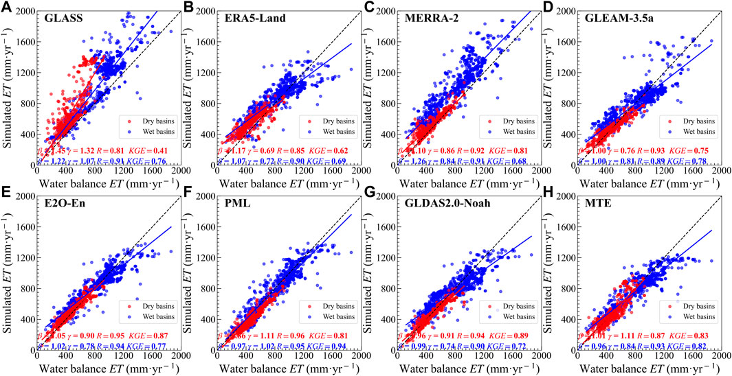
FIGURE 4. Scatterplots of water balance ET versus ET simulated by ET products for wet and dry basins, accompanied by various validation criteria (KGE and its components R, $\beta$ and $\gamma$) at the bottom of each panel. (A–H) represent the GLASS, ERA5-Land, MERRA-2, GLEAM-3.5a, E2O-En, PML, GLDAS2.0-Noah and MTE, respectively. The blue and red represent wet and dry basins, respectively.

With $\beta$ at $\sim$ 1.0, the magnitude of temporal variability of ET tended to be more easily simulated under dry condition, compared with wet condition (Figure 5). As for $\gamma$, the spatial variability of ET temporal variability was generally overestimated by ET products under all aridity conditions, with 0.87 for GLDAS2.0-Noah≤ $\gamma$ ≤1.47 for ERA5-Land under dry condition, and 0.79 for GLASS≤ $\gamma$ ≤1.95 for PML under wet condition. As for R, the ET products could detect the spatial distribution of ET CV under dry basins, of which the highest R value was 0.76 for MERRA-2, followed by 0.69 for E2O-En. However, under wet condition, the ET products presented a contrasting performance, compared with dry condition, with R values ranging from −0.07 to 0.12. Considering KGE, similar to R, the ET products could not simulate the ET CV under wet condition, whereas, under dry condition, ERA5-land, MERRA-2, GLEAM3.5a, E2O-En and GLDAS2.0-Noah showed better overall performances, generating a KGE above 0.40.

FIGURE 5

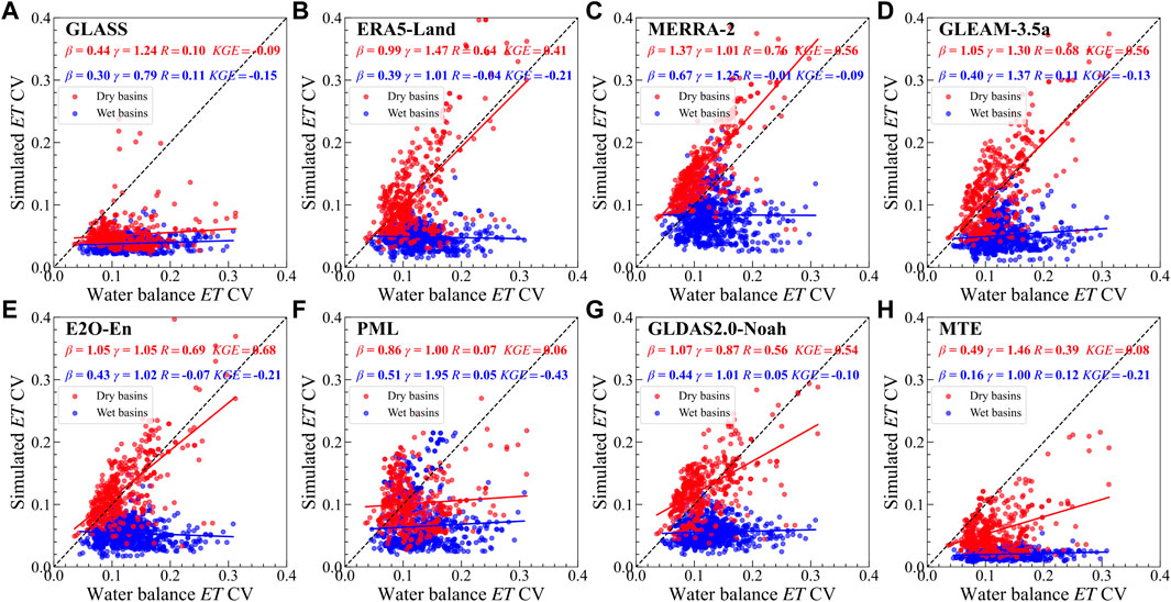
FIGURE 5. Scatterplots of water balance ET CV versus ET CV simulated by ET products for wet and dry basins, accompanied by various validation criteria (KGE and its components R, $\beta$ and $\gamma$) at the top of each panel. (A–H) represent the GLASS, ERA5-Land, MERRA-2, GLEAM-3.5a, E2O-En, PML, GLDAS2.0-Noah and MTE, respectively. The blue and red represent wet and dry basins, respectively.

Taking the ET trend into consideration (Figure 6), more than 50% of the total number of basins were located in the first and third quadrants, with 46.89% for ERA5-Land ≤ TPR + TNR≤78.00% for MERRA-2 under dry condition and 54.20% for GLASS ≤ TPR + TNR≤63.26% for ERA5-Land under wet condition. This indicates that most of the ET products can capture the ET trend directions. Despite that, it is worth noting that FPRs outweighed the TNRs under wet condition. This suggested that under the wet condition, these products tended to change the negative ET trends to the positive ET trends. Based on $\beta$, under wet condition, most of the ET products (except ERA5-Land and MERRA-2) tended to underestimate the magnitude of ET trend, with −19.63 for GLASS≤ $\beta$ ≤-4.93 for GLEAM-3.5a. By contrast, under dry condition, the underestimations of the ET trend got relieved, with −2.06 for ERA5-Land≤ $\beta$ ≤4.76 for GLASS, except that general underestimations still existed in dry condition. In addition, ET products underestimated the extreme ET trends over the wet basins (<−5 and >5 mm yr⁻¹), which mainly occurred in the Amazonian Plain and Brazilian Plateau (Figure 2). As for the spatial variability of ET trend, the $\gamma$ values were around zero for all ET products under wet condition, ranging from −0.09 (GLEAM-3.5a) to 0.18 (ERA5-Land), while the $\gamma$ values were more deviated from optimal value (1.0) for most ET products under dry condition, ranging from −23.21 for GLEAM-3.5a to 23.53 for E2O-En. Overall, all ET products exhibited limited R-based ability to simulate spatial distribution of the ET trend, with 0.09 for GLASS ≤ R ≤ 0.65 for MERRA-2 under dry condition and 0.05 for MTE ≤ R ≤ 0.33 for GLASS under wet condition. Furthermore, the overall performance for each ET product under all aridity conditions was poor with −23.25 (GLEAM-3.5a)≤KGE ≤ 0.44 (MERRA-2) under dry condition and −19.66 (GLASS)≤KGE ≤ −1.05 (ERA5-Land) under wet condition. Notably, the overall performances were generally worse for the latter.

FIGURE 6

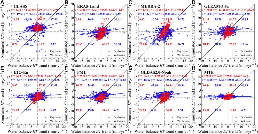
FIGURE 6. Scatterplots of water balance ET trend versus ET trend simulated by ET products for wet and dry basins, accompanied by various validation criteria (KGE and its components R, $\beta$ and $\gamma$) at the top of each panel. (A–H) represent the GLASS, ERA5-Land, MERRA-2, GLEAM-3.5a, E2O-En, PML, GLDAS2.0-Noah and MTE, respectively. The blue and red represent wet and dry basins, respectively. The percentages in the first-fourth quadrants represent the TPR, FPR, TNP, and FNR, respectively. The sum of the percentage values in four quadrants is equal to 100 (%).

Temporally, as shown in Figure 7A, regarding $\beta$, except PML, GLDAS2.0-Noah, and MTE, the magnitudes of ET were overestimated at 51.33% for GLEAM-3.5a to 98.89% for GLASS of dry basins, and at 51.66% for GLEAM-3.5a to 96.46% for MERRA-2 of wet basins. The basin-averaged $\beta$ values for the ET products (except GLASS and MERRA-2) were both near to 1.0 under dry and wet conditions (Figure 7B). The basin-averaged $\gamma$ values under dry condition were also close to 1.0 for most products, while under wet condition the values were overwhelmingly low, ranging from 0.17 for MTE to 0.72 for MERRA-2. As for R (Figure 7C), more than 50% of basins exhibited a value over zero for most products under all conditions. Despite that, each ET product showed a higher R-based ability to simulate ET temporal fluctuation under dry condition than wet condition, with average R values ranging from 0.15 for GLDAS2.0-Noah to 0.46 for MERRA-2 under dry condition and −0.03 for MERRA-2 to 0.17 for ERA5-Land under wet condition. As for KGE (Figure 7D), compared with the R-based ability, the overall performance of ET products under wet conditions worsened. For example, 64.12% (ERA5-Land) to 93.88% (MTE) of basins showed negative KGE values under wet conditions, whereas 63.11% (GLDAS2.0-Noah) to 87.33% (E2O-En) of basins exhibited positive KGE values under dry conditions. Furthermore, all ET products showed a negative average KGE value under wet conditions, while most products, except for GLASS, showed a positive average KGE value under dry conditions.

FIGURE 7

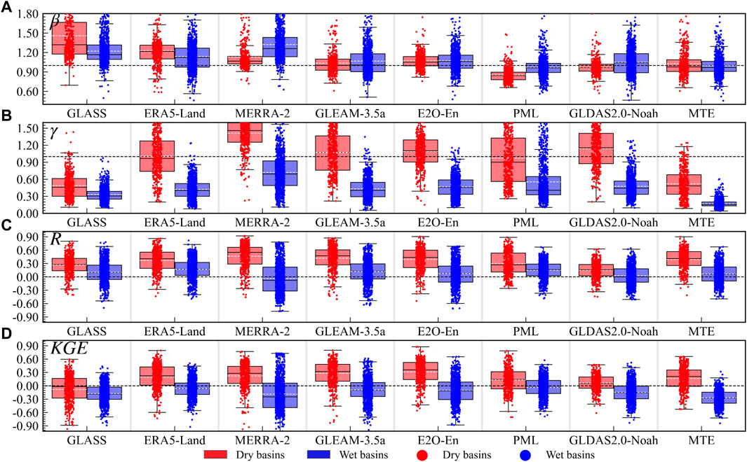
FiGURE 7. Box plots of evaluation metrics for ET products under wet and dry basins. (A–D) represent the KGE and its components R, β and γ, respectively. The blue and red represent wet and dry basins, respectively. The dashed lines represent the average value.

3.3 Validation by vegetation conditions

From perspective of climatological ET, the magnitude and spatial variability of ET could be represented by most of the ET products across all vegetation conditions (Figure 8), with both $\beta$ and $\gamma$ around 1.0. However, most of the ET products (excluding GLASS) also underestimated the ET values above 1,200 mm under LAI-III condition, which mainly exist in Amazonian Plain and Brazilian Plateau (Figure 2). Concerning R, the capacity to simulate the spatial distribution of climatological ET increased first, and then decreased as vegetation became greener for most ET products except GLDAS2.0-Noah, In terms of KGE, most ET products show good KGE-based performance. In addition, GLASS, ERA5-Land, MERRA-2, E2O-En, PML, and MTE showed that the KGE-based performance was the best under LAI-II condition.

FIGURE 8

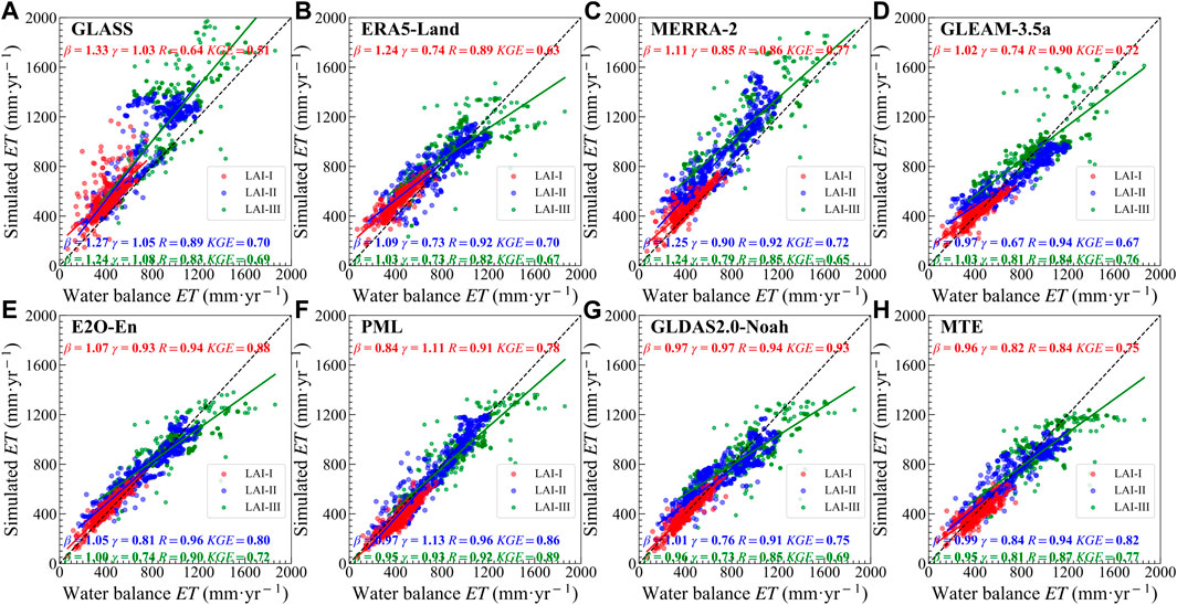
FIGURE 8. Scatterplots of water balance ET CV versus ET CV simulated by ET products under LAI-I, LAI-II, and LAI-III conditions, accompanied by various validation criteria (KGE and its components R, $\beta$ and $\gamma$) at the top of each panel. (A–H) represent the GLASS, ERA5-Land, MERRA-2, GLEAM-3.5a, E2O-En, PML, GLDAS2.0-Noah and MTE, respectively. The red, blue and green represent the vegetation greenness levels of LAI-I (LAI<1), LAI-II (1 ≤ LAI<2) and LAI-III (LAI≥2) respectively.

In terms of the ET CV (Figure 9), most ET products (except GLASS and MTE) reasonably estimated ET magnitude under LAI-I condition, with 0.86 for PML≤ $\beta$ ≤1.34 for ERA5-Land. However, the $\beta$ values were limited for other vegetation conditions, with 0.22 for MTE≤ $\beta$ ≤0.62 for PML under LAI-II condition and 0.14 for PML≤ $\beta$ ≤0.67 for MERRA-2 under LAI-III condition. The $\beta$ values for the ET temporal variability decreased as the vegetation turned green for each ET product. And the $\gamma$ values for the spatial variability of ET temporal variability tended to be overestimated under all vegetation conditions. For R, all the ET products (except PML) had the limited R-based ability to simulate the spatial distribution of ET temporal variability, with vegetation greening. For example, the R values under LAI-I, LAI-II, LAI-III conditions ranged from 0.24 to 0.69, 0.24 to 0.38, and −0.09 to 0.13, respectively. Similar trends were occurred to KGE, except that the overall performance of KGE was even worse than that of R-capacity.

FIGURE 9

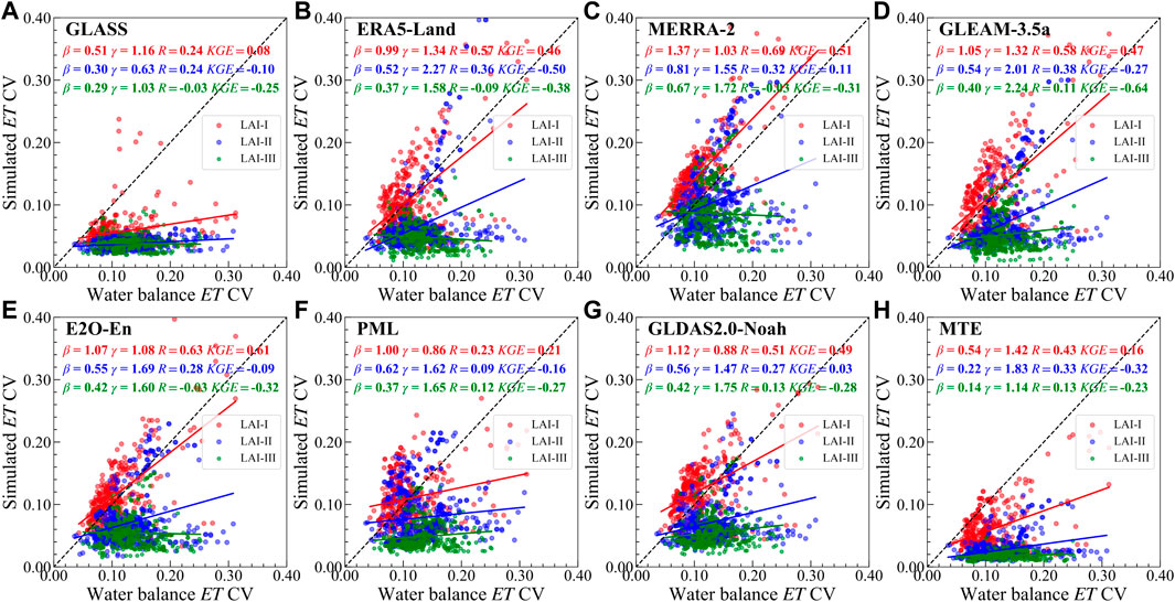
FIGURE 9. Scatterplots of water balance ET CV versus ET CV simulated by ET products under LAI-I, LAI-II, and LAI-III conditions, accompanied by various validation criteria (KGE and its components R, $\mathit{\beta }$ and $\mathit{\gamma }$) at the top of each panel. (A–H) represent the GLASS, ERA5-Land, MERRA-2, GLEAM-3.5a, E2O-En, PML, GLDAS2.0-Noah and MTE, respectively. The red, blue and green represent the vegetation greenness levels of LAI-I (LAI<1), LAI-II (1 ≤ LAI<2) and LAI-III (LAI≥2), respectively.

In the view of ET trend (Figure 10), its condition is similar to the aridity condition. The ET products could hit the ET trend directions, with 50.73% for PML ≤ TPR + TNR79.88% for MERRA-2 under LAI-I condition, 52.58% for GLASS ≤ TPR + TNR≤66.39% for PML under LAI-II condition, and 52.09% for PML ≤ TPR + TNR≤66.85% for ERA5-Land under LAI-III condition. Additionally, FPRs outweighed the TNRs for ET products (except ERA5-Land and MERRA-2) under LAI-II and LAI-III conditions, for example, for GLDAS2.0-Noah, FPR versus TNR was 39.27% versus 8.82% under LAI-II condition, and 40.96% versus 7.32% under LAI-III condition, indicating that the ET products tended to misidentify the negative ET trends as positive ET trends. Based on $\beta$, except ERA5-Land and MERRA-2, the ET products tended to seriously underestimate the magnitudes of ET under LAI-III condition, with −8.21 for GLASS≤ $\beta$ ≤-3.15 for MTE. And the values of $\beta$ were much larger than 1.0 under LAI-II condition (excluding ERA5-Land and MERRA-2), suggesting that the overestimation occurred in LAI-II condition. As for $\gamma$, all the ET products underestimated the spatial variability of the trends (excluding MERRA-2, GLEAM-3.5a, E2O-En and MTE for LAI-I condition). As for R values, the ET products (except GLASS, MTE and PML) showed lower correlations with the greening of vegetation. Interestingly, the ET trends were remarkably overestimated by most products in LAI-II condition, and slightly underestimated under LAI-I and LAI-III conditions. As for KGE, most of the ET products had bad performance with negative values under all conditions. Especially under LAI-II and LAI-III conditions, they had almost no simulability.

FIGURE 10

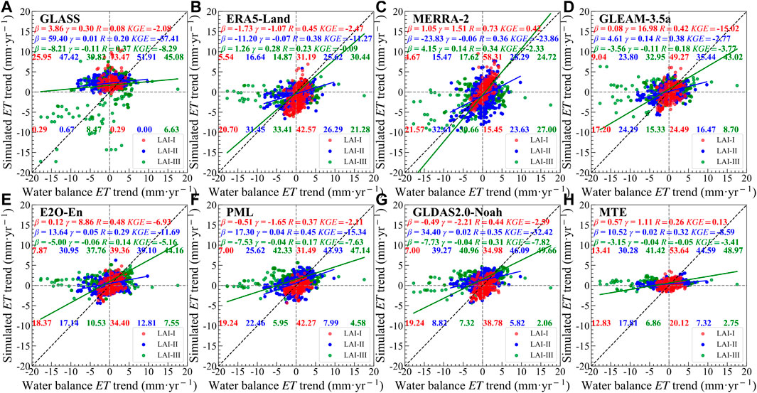
FIGURE 10. Scatterplots of water balance ET trend versus ET trend simulated by ET products under LAI-I, LAI-II, and LAI-III conditions, accompanied by various validation criteria (KGE and its components R, $\beta$ and $\gamma$) at the top of each panel. (A–H) represent the GLASS, ERA5-Land, MERRA-2, GLEAM-3.5a, E2O-En, PML, GLDAS2.0-Noah and MTE, respectively. The red, blue and green represent the vegetation greenness levels of LAI-I (LAI<1), LAI-II (1 ≤ LAI<2) and LAI-III (LAI≥2), respectively. The percentages in the first-fourth quadrants represent the TPR, FPR, TNP, and FNR, respectively. The sum of the percentage values in four quadrants is equal to 100 (%).

Temporally, the basin-averaged $\beta$ values were around the 1.0 for all vegetation conditions (Figure 11A), though the temporal magnitudes of ET were either overestimated or underestimated by the ET products. Considering $\gamma$ (Figure 11B), the basin-averaged values for all the ET products significantly decreased with the vegetation turning green, and were overestimated under LAI-I condition, but underestimated under the other vegetation conditions. It is worth noting that as vegetation was getting greener, the R-based ability for all the ET products was significantly constrained (Figure 11C). Specifically, all the ET products consistently performed, and the average R value and the basin percentages of the R values over zero decreased with vegetation greening. Figure 11D clearly shows that, like R-based ability, the basin-averaged overall performances of all the ET products decreased, as the vegetation was getting greener, except that the KGE values were lower than R values.

FIGURE 11

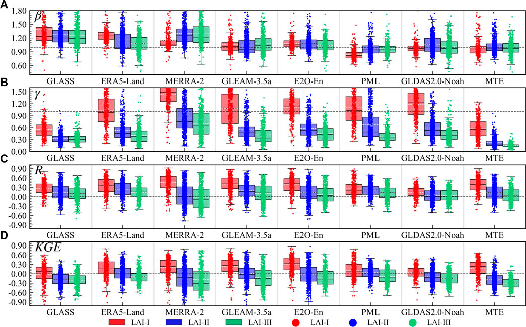
FIGURE 11. Box plots of evaluation metrics for ET products under LAI-I, LAI-II, and LAI-III conditions. (A–D) represent the KGE and its components R, β and γ, respectively. The blue, red and green represent LAI-I, LAI-II, and LAI-III conditions, respectively. The dashed lines represent the basin-averaged value.

4 Discussion

4.1 Validation by dynamic aridity or vegetation conditions

In this study, the simulations of ET derived from the eight methods were evaluated by the water balance ET of global 1,381 basins under various water, energy, and vegetation conditions. Since water, energy, and vegetation are crucial for accurately simulating ET, the lack of sufficient their information, caused by the lack of ET algorithm, forcing data and calibration methods, affects the performance of ET simulation (Xu et al., 2019; Elnashar et al., 2021; Li et al., 2022; Yu et al., 2022). As is shown, the comprehensive performance of ET products (Figures 7, 11) and the capture of ET variance (Figures 5, 9) regularly decrease, with the humidity and vegetation greenness increasing. These phenomena imply that the accuracy of the ET simulations may decrease, when the regional climate is wetting and the global vegetation is greening (Mankin et al., 2017; Lian et al., 2021; Zhang et al., 2022). Additionally, the ET products tend to misidentify the negative trends as the positive trends, especially under wet and LAI-III conditions, implying that the estimates of ET trends may be overestimated across the globe or in wet and LAI-III conditions (Figures 6, 10). These issues will be further discussed in the following.

In terms of the impact of water and energy denoted by AI, ET process in dry or wet regions can be conceptualized as a water- or energy-limited process, respectively: ET under dry conditions is water-limited, in that it is constrained by the soil moisture available for ET, while ET under wet conditions is energy limited, since there is sufficient soil moisture available for ET. Therefore, the maximum rate and temporal variations of ET proceeds are determined by atmospheric water demand (potential evapotranspiration) rather than soil moisture (Draper et al., 2018). All the ET products could better capture the mean annual value of all aridity conditions. However, the ET CV in wet basins tend to be more remarkably underestimated than in dry basins, by the ET products except GLASS and PML (Figures 5, 7). Indeed, wet zones have more active land-atmosphere coupling than dry zones, in that the inevitable ET algorithm errors or data forcing errors magnify the uncertainties under wet zones. For instance, Penman-Monteith method (GLDAS2.0-Noah, MERRA-2 and PML) is primarily driven by net radiation (R_n) under wet zones using a linearized approximate solution (Gao, 1988; Grignon, 1992; Leca et al., 2011), which is sensitive to low vapor pressure deficit (VPD) and may induce considerable problems in the extreme conditions (such as the water balance ET higher 1,200 mm (Figure 4) and extreme ET trends (Figure 6) and the soil evaporative term (Bai and Liu, 2018; Blatchford et al., 2020). More importantly, the presence or absence of ET products TWSC components in simulating ET under dry and wet areas cannot be ignored. However, most ET methods do not have an aquifer storage component, and LSMs lack a good representation of groundwater withdrawal for agricultural depletion, such as irrigation (Liu et al., 2016; Zeng and Cai, 2018). Additionally, the errors in the ET estimates and differences among the ET products are also mainly dependent on various inputs (Li et al., 2018).

The surface variables also control the ET process, especially vegetation (Wang et al., 2022; Zheng et al., 2022). Similarly, the response of ET products to vegetation was investigated. Regarding the mean annual value, we found that the simulability of datasets first increased and then decreased, with the increase of vegetation density (Figure 8), in line with the Lu et al. (2021). In addition, we also confirmed that the comprehensive performance (KGE) of ET products decreases as the vegetation is getting greener (Figures 8, 10). The first reason for this is that whether ET algorithms take the LAI or vegetation dynamics into consideration. For example, GLEAM-3.5a model lacks vegetation-related information, though it considers the vegetation optical depth, which may result in lower accuracy in high vegetation regions (Martens et al., 2017; Xu et al., 2019; Qiu et al., 2022). Another reason is that the ET algorithm do not comprehensively consider the vegetation process in hydrology or energy cycle. MERRA-2 overestimates the interception loss fraction defined as the fraction of rainfall, i.e., rainfall intercepted by the canopy and reevaporating back into the atmosphere without infiltrating into the soil or causing surface runoff (Reichle et al., 2011; Bosilovich et al., 2017; Gelaro et al., 2017; Reichle et al., 2017; Hinkelman, 2019), which could explain why the MERRA-2 generally has the highest $\beta$ under various LAI conditions among the eight ET products (Figures 8, 11, and Lv et al. (2020)). The last easily neglected issue is related to the model forcing data. One aspect of the issue is the forcing data errors. The accuracy of LAI dataset is impacted by the leaf shadowing (Mehrez et al., 1992), especially tall and dense vegetations. Besides, shaded leaves are not light-saturated, leading to diffuse sunlight conditions and then having a higher fraction of FAPAR (the fraction of photosynthetically active radiation absorbed by the canopy) (Jimenez et al., 2011; He et al., 2013; Xu et al., 2019). Another aspect of the issue is the forcing data settings, for instance, MTE ET product was generated from machine learning method by compiling the 253 globally distributed flux towers data and remote sensing data, including vegetation information (FAPAR). We speculated that the varying performance of MTE product with various LAI conditions was probably driven by data settings. For example, the vegetation was used to do split not regression, which results in inadequate vegetation information (Jung et al., 2010). Or ERA5-Land was used to generate land elements data including ET, by using a static monthly climatology of a fixed land use and leaf area index (LAI) (Muñoz-Sabater et al., 2021). And GLDAS2.0-Noah also uses a static land use, though with high spatial resolution (Rodell et al., 2004). Therefore, they ignored the change of land cover and cities, and lost more frequent LAI anomalies during the reanalysis period (Muñoz-Sabater et al., 2021).

The model calibration methods also have a significant impact on the performance of ET simulation. One problem concerning the methods is that the ET simulations are often calibrated with the mean annual value not the variance and trend of actual ET, though considering multiple calibration metrics. Another problem is that the data used for calibration are often EC site data that are not representative of the regional scale (Bai and Liu, 2018; Xu et al., 2019). In addition, as far as we know, the ET products except GLASS and MTE are accompanied by component data such as soil evaporation, vegetation evapotranspiration and water surface evaporation, but these data are not calibrated with sufficient actual measurements (Swanson, 1994; Brunel et al., 1997; Chen et al., 2014).

4.2 Uncertainties

The uncertainties in Pre and TWSA products are the largest source of uncertainties in assessing the ET products (Liu et al., 2016). According to the water balance budget, the assessment of global-scale ET products needs to rely on grid-scale Pre and TWSA products, although the global-scale observatory data is difficult to collect. As for the three Pre products selected in this study (GPCC, CPC-Unified, and CRU TS4.05), the uncertainties derive from the number of stations used, the time homogeneity and the quality control procedures (Trenberth et al., 2014; Sun et al., 2018). However, these products are interpolated from an unprecedented number of station data and are the most reliable precipitation products currently available (Sun et al., 2018). Regarding the TWSA data (GRACE-REC and GRID-CSR-GRACE-REC), the uncertainties arise mainly from the models used for the reconstruction (pre-2002) and the driving data (Gyawali et al., 2022). However, the correlation of GRACE-REC with yearly streamflow anomalies have median value of around 0.60 over 1981–2010 (Humphrey and Gudmundsson, 2019); the GRID-CSR-GRACE-REC has high correlation with Global Mean Sea level with R of 0.91 (Li et al., 2021). We further investigated the uncertainties in water balance evapotranspiration defined as the CV of the six Pre-TWSC-Q combinations, and found that most of the basins with uncertainties of <0.10 and uncertainties above 0.10 were located mainly in the Midwest USA and Southwest China (rainfall gauges are more sparsely distributed in high mountain areas) and the Arctic (Figure 12). In addition, Q data may be affected by human harvesting of deep groundwater and inter-basin water transfers (Liu et al., 2016). However, TWSC can reasonably take into account the impact of human activities on Q. Moreover, in validating the model, only the terrestrial water balance (not the atmospheric water balance) is considered, and the measured evapotranspiration values lack the cross-validation to further reduce the error with the true values (Li et al., 2019). The generalizability of our results to other regions of the world may be subject to additional uncertainty, as the basins included in this study do not cover the entire globe. However, it is important to note that the performance of evapotranspiration products varies with dryness and vegetation greenness, and it is necessary to ensure that all types of dryness and vegetation greenness are covered (Figure 1). To minimize errors caused by different spatial resolutions, all ET products were re-interpolated linearly to 0.5° before evaluation. Furthermore, our analysis is based on observed ET using the water balance method, which represents the average ET of watersheds controlled by hydrological stations, reducing the uncertainty caused by a single grid point to some extent. The scale effect on ET product performance related to aridity and vegetation greenness response needs further exploration in future research.

FIGURE 12

FIGURE 12. Spatial pattern of uncertainties of water balance ET at global 1,381 basins. The histogram presents uncertainty values at different levels corresponding to the color bars.

5 Conclusion

This study conducted a comprehensive assessment of terrestrial ET products to improve ET products. In this study, drawing on the data of water balance ET from 1981–2010 collected from 1,381 basins, we examined eight ET products: one remote sensing product (GLASS), two reanalysis products (ERA5-Land and MERRA-2), four LSM-based products (GLEAM-3.5a, E2O-En, PML and GLDAS2.0-Noah), and one machine learning-based product (MTE). Besides, to gain a deeper insight into the eight ET estimates under various conditions, the potential impact of aridity and vegetation greenness were taken in consideration. The evaluation results are summarized below:

(1) In view of the performance at the global scale, the ET products had advantages in capturing the mean annual value of ET, with relatively high KGE values, among which the PML performed the best with 0.89 for KGE. Despite that, the ET products had limited KGE-ability to simulate the ET variability with highest KGE of 0.04 for MERRA-2 and the trend with highest KGE of −1.47 for GLEAM-3.5a. In addition, the ET products tended to underestimate the ET temporal variability and overestimate its spatial dynamics, while they tended to overestimate the ET trend and underestimate its spatial dynamics. It is worth noting that the ET products tended to misidentify the negative ET trend as positive trend.

(2) For each basin, the ET products always overestimated the ET values and underestimated the ET temporal variability at more than 50% of basins. And the ET products had a wide R-based ability to simulate the ET temporal fluctuation, for the ET products had positive R values at 59.30% (MERRA-2)—84.50% (ERA5-Land) of basins. The high R values mainly appeared in the Midwest United States, South Africa, Western Australia. However, all ET products showed the limited KGE-ability at the temporal scale.

(3) As for different aridity regimes, the performances of ET products were completely opposite in dry and wet areas. Spatially, the ET products showed lower ability to capture the temporal variability and the trend of ET under wet condition than dry condition. And overall, the ET products tended to misidentify the negative ET trend as positive trend, which only existed in wet condition. Temporally, the overall performances of ET products were limited under wet condition, for the ET products performed the negative KGE values under wet condition, and the positive KGE values under dry condition at more than 60% of basins.

(4) Considering the dynamic performances with varying vegetation, the spatial and temporal performances of ET products were strongly affected by vegetation greenness, which is similar to the situation with aridity regimes. Spatially, as vegetation became greener, the performance of simulated climatological ET increased first and then decreased, and gradually limited the ability to simulate the spatial distribution of ET temporal variability. Meanwhile, the ET products tended to misidentify the negative ET trend as positive trend under lush vegetation condition. Temporally, the basin-averaged overall performances of all the ET products decreased, as the vegetation was getting greener.

Overall, the performances of ET products were poor in wet or vegetated areas, suggesting that the accuracy of ET products may decline in the future when the climate becomes wetter and the vegetation becomes greener. Therefore, this work is hopefully to improve our understanding about the spatio-temporal performance of the ET products, and contribute to the directional optimizations and effective applications of ET products.

Data availability statement

The raw data supporting the conclusions of this article will be made available by the authors, without undue reservation.

Author contributions

Data curation, HW, CT, YX, and DL; conceptualization, GY, HW, and CT; methodology, HW; visualization, HW, CT, and YX; writing–original draft, HW, writing–review and editing, GY, XL, and CT; investigation, JW, DL, and FY; software, PZ; supervision, GY.

Funding

This study was supported by the National Natural Science Foundation of China (Grant NO. 42075189), the Natural Science Foundation of Jiangsu Province, China (Grant No. BK20200096), Hubei Branch of China National Tobacco Corporation (Grant No. 027Y2021021), and Jiangsu Provincial Bureau of Hydrology and Water Resources Survey (Grant Nos. 2211052001601 and 2211052101801).

Conflict of interest

The authors declare that the research was conducted in the absence of any commercial or financial relationships that could be construed as a potential conflict of interest.

Publisher’s note

All claims expressed in this article are solely those of the authors and do not necessarily represent those of their affiliated organizations, or those of the publisher, the editors and the reviewers. Any product that may be evaluated in this article, or claim that may be made by its manufacturer, is not guaranteed or endorsed by the publisher.

References

Albergel, C., Dutra, E., Munier, S., Calvet, J.-C., Munoz-Sabater, J., De Rosnay, P., et al. (2018). ERA-5 and ERA-interim driven ISBA land surface model simulations: Which one performs better? Hydrology Earth Syst. Sci. 22, 3515–3532. doi:10.5194/hess-22-3515-2018

CrossRef Full Text | Google Scholar

Alemohammad, S. H., Fang, B., Konings, A. G., Aires, F., Green, J. K., Kolassa, J., et al. (2017). Water, energy, and carbon with artificial neural networks (WECANN): A statistically based estimate of global surface turbulent fluxes and gross primary productivity using solar-induced fluorescence. Biogeosciences 14, 4101–4124. doi:10.5194/bg-14-4101-2017

PubMed Abstract | CrossRef Full Text | Google Scholar

Almagro, A., Oliveira, P. T. S., Meira Neto, A. A., Roy, T., Troch, P. J. H., and Sciences, E. S. (2021). CABra: A novel large-sample dataset for Brazilian catchments. Hydrology Earth Syst. Sci. 25, 3105–3135. doi:10.5194/hess-25-3105-2021

CrossRef Full Text | Google Scholar

Arsenault, R., Bazile, R., Ouellet Dallaire, C., and Brissette, F. J. H. P. (2016). Canopex: A Canadian hydrometeorological watershed database. Hydrol. Process. 30, 2734–2736. doi:10.1002/hyp.10880

CrossRef Full Text | Google Scholar

Arsenault, R., Brissette, F., Martel, J.-L., Troin, M., Lévesque, G., Davidson-Chaput, J., et al. (2020). A comprehensive, multisource database for hydrometeorological modeling of 14,425 North American watersheds. Sci. Data 7, 243–312. doi:10.1038/s41597-020-00583-2

PubMed Abstract | CrossRef Full Text | Google Scholar

Awange, J., Hu, K., and Khaki, M. (2019). The newly merged satellite remotely sensed, gauge and reanalysis-based Multi-Source Weighted-Ensemble Precipitation: Evaluation over Australia and Africa (1981–2016). Sci. total Environ. 670, 448–465. doi:10.1016/j.scitotenv.2019.03.148

PubMed Abstract | CrossRef Full Text | Google Scholar

Badgley, G., Fisher, J. B., Jiménez, C., Tu, K. P., and Vinukollu, R. (2015). On uncertainty in global terrestrial evapotranspiration estimates from choice of input forcing datasets. J. Hydrometeorol. 16, 1449–1455. doi:10.1175/JHM-D-14-0040.1

CrossRef Full Text | Google Scholar

Bai, P., and Liu, X. (2018). Intercomparison and evaluation of three global high-resolution evapotranspiration products across China. J. hydrology 566, 743–755. doi:10.1016/j.jhydrol.2018.09.065

CrossRef Full Text | Google Scholar

Beck, H. E., De Roo, A., and Van Dijk, A. I. (2015). Global maps of streamflow characteristics based on observations from several thousand catchments. J. Hydrometeorol. 16, 1478–1501. doi:10.1175/JHM-D-14-0155.1

CrossRef Full Text | Google Scholar

Becker, A., Finger, P., Meyer-Christoffer, A., Rudolf, B., Schamm, K., Schneider, U., et al. (2013). A description of the global land-surface precipitation data products of the Global Precipitation Climatology Centre with sample applications including centennial (trend) analysis from 1901–present. Earth Syst. Sci. Data 5, 71–99. doi:10.5194/essd-5-71-2013

CrossRef Full Text | Google Scholar

Blatchford, M. L., Mannaerts, C. M., Njuki, S. M., Nouri, H., Zeng, Y., Pelgrum, H., et al. (2020). Evaluation of WaPOR V2 evapotranspiration products across Africa. Hydrol. Process. 34, 3200–3221. doi:10.1002/hyp.13791

CrossRef Full Text | Google Scholar

Bosilovich, M. G., Robertson, F. R., Takacs, L., Molod, A., and Mocko, D. (2017). Atmospheric water balance and variability in the MERRA-2 reanalysis. J. Clim. 30, 1177–1196. doi:10.1175/JCLI-D-16-0338.1

CrossRef Full Text | Google Scholar

Brunel, J.-P., Walker, G., Dighton, J., and Monteny, B. (1997). Use of stable isotopes of water to determine the origin of water used by the vegetation and to partition evapotranspiration. A case study from HAPEX-Sahel. J. hydrology 188, 466–481. doi:10.1016/S0022-1694(96)03188-5

CrossRef Full Text | Google Scholar

Chagas, V. B., Chaffe, P. L., Addor, N., Fan, F. M., Fleischmann, A. S., Paiva, R. C., et al. (2020). CAMELS-BR: Hydrometeorological time series and landscape attributes for 897 catchments in Brazil. Earth Syst. Sci. Data 12, 2075–2096. doi:10.5194/essd-12-2075-2020

CrossRef Full Text | Google Scholar

Chen, M., Shi, W., Xie, P., Silva, V. B., Kousky, V. E., Wayne Higgins, R., et al. (2008). Assessing objective techniques for gauge-based analyses of global daily precipitation. J. Geophys. Res. Atmos. 113, D04110–D04113. doi:10.1029/2007JD009132

CrossRef Full Text | Google Scholar

Chen, Y., Xia, J., Liang, S., Feng, J., Fisher, J. B., Li, X., et al. (2014). Comparison of satellite-based evapotranspiration models over terrestrial ecosystems in China. Remote Sens. Environ. 140, 279–293. doi:10.1016/j.rse.2013.08.045

CrossRef Full Text | Google Scholar

Coxon, G., Addor, N., Bloomfield, J. P., Freer, J., Fry, M., Hannaford, J., et al. (2020). CAMELS-GB: Hydrometeorological time series and landscape attributes for 671 catchments in Great Britain. Earth Syst. Sci. Data 12, 2459–2483. doi:10.5194/essd-12-2459-2020

CrossRef Full Text | Google Scholar

Draper, C. S., Reichle, R. H., and Koster, R. D. (2018). Assessment of MERRA-2 land surface energy flux estimates. J. Clim. 31, 671–691. doi:10.1175/JCLI-D-17-0121.1

CrossRef Full Text | Google Scholar

Elnashar, A., Wang, L., Wu, B., Zhu, W., and Zeng, H. (2021). Synthesis of global actual evapotranspiration from 1982 to 2019. Earth Syst. Sci. Data 13, 447–480. doi:10.5194/essd-13-447-2021

CrossRef Full Text | Google Scholar

Ershadi, A., Mccabe, M., Evans, J. P., Chaney, N. W., and Wood, E. F. (2014). Multi-site evaluation of terrestrial evaporation models using FLUXNET data. Agric. For. Meteorology 187, 46–61. doi:10.1016/j.agrformet.2013.11.008

CrossRef Full Text | Google Scholar

Fisher, J. B., Tu, K. P., and Baldocchi, D. D. (2008). Global estimates of the land–atmosphere water flux based on monthly AVHRR and ISLSCP-II data, validated at 16 FLUXNET sites. Remote Sens. Environ. 112, 901–919. doi:10.1016/j.rse.2007.06.025

CrossRef Full Text | Google Scholar

Fowler, K. J., Acharya, S. C., Addor, N., Chou, C., and Peel, M. C. J. E. S. S. D. (2021). CAMELS-AUS: Hydrometeorological time series and landscape attributes for 222 catchments in Australia. Earth Syst. Sci. Data 13, 3847–3867. doi:10.5194/essd-13-3847-2021

CrossRef Full Text | Google Scholar

Gao, G., Fu, B., Wang, S., Liang, W., and Jiang, X. (2016). Determining the hydrological responses to climate variability and land use/cover change in the Loess Plateau with the Budyko framework. Sci. Total Environ. 557, 331–342. doi:10.1016/j.scitotenv.2016.03.019

PubMed Abstract | CrossRef Full Text | Google Scholar

Gao, W. (1988). Applications of solutions to non-linear energy budget equations. Agric. For. Meteorology 43, 121–145. doi:10.1016/0168-1923(88)90087-1

CrossRef Full Text | Google Scholar

Gelaro, R., Mccarty, W., Suárez, M. J., Todling, R., Molod, A., Takacs, L., et al. (2017). The modern-era retrospective analysis for research and applications, version 2 (MERRA-2). J. Clim. 30, 5419–5454. doi:10.1175/JCLI-D-16-0758.1

CrossRef Full Text | Google Scholar

Gobron, N., Pinty, B., Aussedat, O., Chen, J. M., Cohen, W. B., Fensholt, R., et al. (2006). Evaluation of fraction of absorbed photosynthetically active radiation products for different canopy radiation transfer regimes: Methodology and results using Joint Research Center products derived from SeaWiFS against ground-based estimations. J. Geophys. Res. Atmos. 111, D13110–D13115. doi:10.1029/2005JD006511

CrossRef Full Text | Google Scholar

Gobron, N., Pinty, B., Aussedat, O., Taberner, M., Faber, O., Mélin, F., et al. (2008). Uncertainty estimates for the FAPAR operational products derived from MERIS—impact of top-of-atmosphere radiance uncertainties and validation with field data. Remote Sens. Environ. 112, 1871–1883. doi:10.1016/j.rse.2007.09.011

CrossRef Full Text | Google Scholar

Grignon, F. (1992). A discussion of the Penman form equations and comparisons of some equations to estimate latent energy flux density. Agric. For. meteorology 57, 297–304. doi:10.1016/0168-1923(92)90125-N

CrossRef Full Text | Google Scholar

Gu, L., Chen, J., Yin, J., Xu, C. Y., and Zhou, J. (2020). Responses of precipitation and runoff to climate warming and implications for future drought changes in China. Earth's Future 8, e2020EF001718. doi:10.1029/2020EF001718

CrossRef Full Text | Google Scholar

Gyawali, B., Ahmed, M., Murgulet, D., and Wiese, D. N. (2022). Filling temporal gaps within and between GRACE and GRACE-FO terrestrial water storage records: An innovative approach. Remote Sens. 14, 1565. doi:10.3390/rs14071565

CrossRef Full Text | Google Scholar

Han, S.-C., Shum, C., and Braun, A. (2005). High-resolution continental water storage recovery from low–low satellite-to-satellite tracking. J. Geodyn. 39, 11–28. doi:10.1016/j.jog.2004.08.002

CrossRef Full Text | Google Scholar

He, M., Ju, W., Zhou, Y., Chen, J., He, H., Wang, S., et al. (2013). Development of a two-leaf light use efficiency model for improving the calculation of terrestrial gross primary productivity. Agric. For. meteorology 173, 28–39. doi:10.1016/j.agrformet.2013.01.003

CrossRef Full Text | Google Scholar

Hinkelman, L. M. (2019). The global radiative energy budget in MERRA and MERRA-2: Evaluation with respect to CERES EBAF data. J. Clim. 32, 1973–1994. doi:10.1175/JCLI-D-18-0445.1

CrossRef Full Text | Google Scholar

Holmes, R. M., Coe, M. T., Fiske, G. J., Gurtovaya, T., Mcclelland, J. W., Shiklomanov, A. I., et al. (2013). “Climate change impacts on the hydrology and biogeochemistry of Arctic rivers,” in Climatic change and global warming of inland waters (Hoboken, New Jersey, United States: Wiley), 1–26. doi:10.1002/9781118470596.ch1

CrossRef Full Text | Google Scholar

Humphrey, V., and Gudmundsson, L. J. E. S. S. D. (2019). GRACE-REC: A reconstruction of climate-driven water storage changes over the last century. Earth Syst. Sci. Data 11, 1153–1170. doi:10.5194/essd-11-1153-2019

CrossRef Full Text | Google Scholar

Jimenez, C., Prigent, C., Mueller, B., Seneviratne, S. I., Mccabe, M., Wood, E. F., et al. (2011). Global intercomparison of 12 land surface heat flux estimates. J. Geophys. Res. Atmos. 116, D02102–D02127. doi:10.1029/2010JD014545

CrossRef Full Text | Google Scholar

Jing, W., Di, L., Zhao, X., Yao, L., Xia, X., Liu, Y., et al. (2020a). A data-driven approach to generate past GRACE-like terrestrial water storage solution by calibrating the land surface model simulations. Adv. Water Resour. 143, 103683. doi:10.1016/j.advwatres.2020.103683

CrossRef Full Text | Google Scholar

Jing, W., Zhang, P., Zhao, X., Yang, Y., Jiang, H., Xu, J., et al. (2020b). Extending GRACE terrestrial water storage anomalies by combining the random forest regression and a spatially moving window structure. J. Hydrology 590, 125239. doi:10.1016/j.jhydrol.2020.125239

CrossRef Full Text | Google Scholar

Jung, H. C., Getirana, A., Policelli, F., Mcnally, A., Arsenault, K. R., Kumar, S., et al. (2017). Upper Blue Nile basin water budget from a multi-model perspective. J. hydrology 555, 535–546. doi:10.1016/j.jhydrol.2017.10.040

CrossRef Full Text | Google Scholar

Jung, M., Reichstein, M., and Bondeau, A. J. B. (2009). Towards global empirical upscaling of FLUXNET eddy covariance observations: Validation of a model tree ensemble approach using a biosphere model. Biogeosciences 6, 2001–2013. doi:10.5194/bg-6-2001-2009

CrossRef Full Text | Google Scholar

Jung, M., Reichstein, M., Ciais, P., Seneviratne, S. I., Sheffield, J., Goulden, M. L., et al. (2010). Recent decline in the global land evapotranspiration trend due to limited moisture supply. Nature 467, 951–954. doi:10.1038/nature09396

PubMed Abstract | CrossRef Full Text | Google Scholar

Kim, H. W., Hwang, K., Mu, Q., Lee, S. O., and Choi, M. (2012). Validation of MODIS 16 global terrestrial evapotranspiration products in various climates and land cover types in Asia. KSCE J. Civ. Eng. 16, 229–238. doi:10.1007/s12205-012-0006-1

CrossRef Full Text | Google Scholar

Kling, H., Fuchs, M., and Paulin, M. (2012). Runoff conditions in the upper Danube basin under an ensemble of climate change scenarios. J. hydrology 424, 264–277. doi:10.1016/j.jhydrol.2012.01.011

CrossRef Full Text | Google Scholar

Klingler, C., Schulz, K., and Herrnegger, M. J. Ö. W.-U. A. (2021). LamaH | Large-Sample Data for Hydrology: Big data für die Hydrologie und Umweltwissenschaften. Österreichische Wasser- Abfallwirtsch. 73, 244–269. doi:10.1007/s00506-021-00769-x

CrossRef Full Text | Google Scholar

Landerer, F. W., and Swenson, S. (2012). Accuracy of scaled GRACE terrestrial water storage estimates. Water Resour. Res. 48, 1–11. doi:10.1029/2011WR011453

CrossRef Full Text | Google Scholar

Leca, A., Parisi, L., Lacointe, A., and Saudreau, M. (2011). Comparison of Penman–Monteith and non-linear energy balance approaches for estimating leaf wetness duration and apple scab infection. Agric. For. meteorology 151, 1158–1162. doi:10.1016/j.agrformet.2011.04.010

CrossRef Full Text | Google Scholar

Li, C., Yang, H., Yang, W., Liu, Z., Jia, Y., Li, S., et al. (2022). Camele: Collocation-analyzed multi-source ensembled land evapotranspiration data. Earth Syst. Sci. Data Discuss. 2022, 1–45. doi:10.5194/essd-2021-456

CrossRef Full Text | Google Scholar

Li, F., Kusche, J., Chao, N., Wang, Z., and Löcher, A. (2021). Long-Term (1979-Present) total water storage anomalies over the global land derived by reconstructing GRACE data. Geophys. Res. Lett. 48, e2021GL093492. doi:10.1029/2021GL093492

CrossRef Full Text | Google Scholar

Li, S., Wang, G., Sun, S., Chen, H., Bai, P., Zhou, S., et al. (2018). Assessment of multi-source evapotranspiration products over China using eddy covariance observations. Remote Sens. 10, 1692. doi:10.3390/rs10111692

CrossRef Full Text | Google Scholar

Li, X., Long, D., Han, Z., Scanlon, B. R., Sun, Z., Han, P., et al. (2019). Evapotranspiration estimation for Tibetan Plateau headwaters using conjoint terrestrial and atmospheric water balances and multisource remote sensing. Water Resour. Res. 55, 8608–8630. doi:10.1029/2019WR025196

CrossRef Full Text | Google Scholar

Lian, X., Piao, S., Chen, A., Huntingford, C., Fu, B., Li, L. Z., et al. (2021). Multifaceted characteristics of dryland aridity changes in a warming world. Nat. Rev. Earth Environ. 2, 232–250. doi:10.1038/s43017-021-00144-0

CrossRef Full Text | Google Scholar

Liu, J., You, Y., Zhang, Q., and Gu, X. (2021). Attribution of streamflow changes across the globe based on the Budyko framework. Sci. Total Environ. 794, 148662. doi:10.1016/j.scitotenv.2021.148662

PubMed Abstract | CrossRef Full Text | Google Scholar

Liu, W., Wang, L., Zhou, J., Li, Y., Sun, F., Fu, G., et al. (2016). A worldwide evaluation of basin-scale evapotranspiration estimates against the water balance method. J. Hydrology 538, 82–95. doi:10.1016/j.jhydrol.2016.04.006

CrossRef Full Text | Google Scholar

Long, D., Shen, Y., Sun, A., Hong, Y., Longuevergne, L., Yang, Y., et al. (2014). Drought and flood monitoring for a large karst plateau in Southwest China using extended GRACE data. Remote Sens. Environ. 155, 145–160. doi:10.1016/j.rse.2014.08.006

CrossRef Full Text | Google Scholar

Lu, J., Wang, G., Chen, T., Li, S., Hagan, D. F. T., Kattel, G., et al. (2021). A harmonized global land evaporation dataset from model-based products covering 1980–2017. Earth Syst. Sci. Data 13, 5879–5898. doi:10.5194/essd-13-5879-2021

CrossRef Full Text | Google Scholar

Lv, M., Xu, Z., and Lv, M. (2020). Evaluating hydrological processes of the atmosphere–vegetation interaction model and MERRA-2 at global scale. Atmosphere 12, 16. doi:10.3390/atmos12010016

CrossRef Full Text | Google Scholar

Majozi, N. P., Mannaerts, C. M., Ramoelo, A., Mathieu, R., Mudau, A. E., and Verhoef, W. (2017). An intercomparison of satellite-based daily evapotranspiration estimates under different eco-climatic regions in South Africa. Remote Sens. 9, 307. doi:10.3390/rs9040307

CrossRef Full Text | Google Scholar

Mankin, J. S., Smerdon, J. E., Cook, B. I., Williams, A. P., and Seager, R. (2017). The curious case of projected twenty-first-century drying but greening in the American West. J. Clim. 30, 8689–8710. doi:10.1175/JCLI-D-17-0213.1

PubMed Abstract | CrossRef Full Text | Google Scholar

Mao, J., Fu, W., Shi, X., Ricciuto, D. M., Fisher, J. B., Dickinson, R. E., et al. (2015). Disentangling climatic and anthropogenic controls on global terrestrial evapotranspiration trends. Environ. Res. Lett. 10, 094008. doi:10.1088/1748-9326/10/9/094008

CrossRef Full Text | Google Scholar

Martens, B., Miralles, D. G., Lievens, H., Van Der Schalie, R., De Jeu, R. A., Fernández-Prieto, D., et al. (2017). GLEAM v3: Satellite-based land evaporation and root-zone soil moisture. Geosci. Model Dev. 10, 1903–1925. doi:10.5194/gmd-10-1903-2017

CrossRef Full Text | Google Scholar

Mccabe, M. F., Ershadi, A., Jimenez, C., Miralles, D. G., Michel, D., and Wood, E. F. (2016). The GEWEX LandFlux project: Evaluation of model evaporation using tower-based and globally gridded forcing data. Geosci. Model Dev. 9, 283–305. doi:10.5194/gmd-9-283-2016

CrossRef Full Text | Google Scholar

Mehrez, M. B., Taconet, O., Vidal-Madjar, D., and Valencogne, C. (1992). Estimation of stomatal resistance and canopy evaporation during the HAPEX-MOBILHY experiment. Agric. For. Meteorology 58, 285–313. doi:10.1016/0168-1923(92)90066-D

CrossRef Full Text | Google Scholar

Miao, Y., and Wang, A. (2020). A daily 0.25°× 0.25° hydrologically based land surface flux dataset for conterminous China, 1961–2017. J. Hydrology 590, 125413. doi:10.1016/j.jhydrol.2020.125413

CrossRef Full Text | Google Scholar

Michel, D., Jiménez, C., Miralles, D. G., Jung, M., Hirschi, M., Ershadi, A., et al. (2016). The WACMOS-ET project–Part 1: Tower-scale evaluation of four remote-sensing-based evapotranspiration algorithms. Hydrology Earth Syst. Sci. 20, 803–822. doi:10.5194/hess-20-803-2016

CrossRef Full Text | Google Scholar

Miralles, D. G., Jiménez, C., Jung, M., Michel, D., Ershadi, A., Mccabe, M., et al. (2016). The WACMOS-ET project–Part 2: Evaluation of global terrestrial evaporation data sets. Hydrology Earth Syst. Sci. 20, 823–842. doi:10.5194/hess-20-823-2016

CrossRef Full Text | Google Scholar

Mu, Q., Heinsch, F. A., Zhao, M., and Running, S. W. (2007). Development of a global evapotranspiration algorithm based on MODIS and global meteorology data. Remote Sens. Environ. 111, 519–536. doi:10.1016/j.rse.2007.04.015

CrossRef Full Text | Google Scholar

Mu, Q., Zhao, M., and Running, S. W. (2011). Improvements to a MODIS global terrestrial evapotranspiration algorithm. Remote Sens. Environ. 115, 1781–1800. doi:10.1016/j.rse.2011.02.019

CrossRef Full Text | Google Scholar

Muñoz-Sabater, J., Dutra, E., Agustí-Panareda, A., Albergel, C., Arduini, G., Balsamo, G., et al. (2021). ERA5-Land: A state-of-the-art global reanalysis dataset for land applications. Earth Syst. Sci. Data 13, 4349–4383. doi:10.5194/essd-13-4349-2021

CrossRef Full Text | Google Scholar

Pan, S., Pan, N., Tian, H., Friedlingstein, P., Sitch, S., Shi, H., et al. (2020). Evaluation of global terrestrial evapotranspiration using state-of-the-art approaches in remote sensing, machine learning and land surface modeling. Hydrology Earth Syst. Sci. 24, 1485–1509. doi:10.5194/hess-24-1485-2020

CrossRef Full Text | Google Scholar

Penman, H. L. (1948). Natural evaporation from open water, hare soil and grass. Math. Phys. Sci. 193, 120–145. doi:10.1098/rspa.1948.0037

CrossRef Full Text | Google Scholar

Priestley, C. H. B., and Taylor, R. J. (1972). On the assessment of surface heat flux and evaporation using large-scale parameters. Mon. weather Rev. 100, 81–92. doi:10.1175/1520-0493(1972)100<0081:OTAOSH>2.3.CO;2

CrossRef Full Text | Google Scholar

Qiu, J., Crow, W. T., Wang, S., Dong, J., Li, Y., Garcia, M., et al. (2022). Microwave-based soil moisture improves estimates of vegetation response to drought in China. Sci. Total Environ. 849, 157535. doi:10.1016/j.scitotenv.2022.157535

PubMed Abstract | CrossRef Full Text | Google Scholar

Reichle, R. H., Draper, C. S., Liu, Q., Girotto, M., Mahanama, S. P., Koster, R. D., et al. (2017). Assessment of MERRA-2 land surface hydrology estimates. J. Clim. 30, 2937–2960. doi:10.1175/JCLI-D-16-0720.1

CrossRef Full Text | Google Scholar

Reichle, R. H., Koster, R. D., De Lannoy, G. J., Forman, B. A., Liu, Q., Mahanama, S. P., et al. (2011). Assessment and enhancement of MERRA land surface hydrology estimates. J. Clim. 24, 6322–6338. doi:10.1175/JCLI-D-10-05033.1

CrossRef Full Text | Google Scholar

Rodell, M., Houser, P., Jambor, U., Gottschalck, J., Mitchell, K., Meng, C.-J., et al. (2004). The global land data assimilation system. Bull. Am. Meteorological Soc. 85, 381–394. doi:10.1175/BAMS-85-3-381

CrossRef Full Text | Google Scholar

Rodell, M., Mcwilliams, E. B., Famiglietti, J. S., Beaudoing, H. K., and Nigro, J. (2011). Estimating evapotranspiration using an observation based terrestrial water budget. Hydrol. Process. 25, 4082–4092. doi:10.1002/hyp.8369

CrossRef Full Text | Google Scholar

Schellekens, J., Dutra, E., Martínez-De La Torre, A., Balsamo, G., Van Dijk, A., Sperna Weiland, F., et al. (2017). A global water resources ensemble of hydrological models: The eartH2Observe tier-1 dataset. Earth Syst. Sci. Data 9, 389–413. doi:10.5194/essd-9-389-2017

CrossRef Full Text | Google Scholar

She, D., Xia, J., and Zhang, Y. (2017). Changes in reference evapotranspiration and its driving factors in the middle reaches of Yellow River Basin, China. Sci. Total Environ. 607, 1151–1162. doi:10.1016/j.scitotenv.2017.07.007

PubMed Abstract | CrossRef Full Text | Google Scholar

Su, Z. (2002). The Surface Energy Balance System (SEBS) for estimation of turbulent heat fluxes. Hydrology earth Syst. Sci. 6, 85–100. doi:10.5194/hess-6-85-2002

CrossRef Full Text | Google Scholar

Sun, Q., Miao, C., Duan, Q., Ashouri, H., Sorooshian, S., and Hsu, K. L. (2018). A review of global precipitation data sets: Data sources, estimation, and intercomparisons. Rev. Geophys. 56, 79–107. doi:10.1002/2017RG000574

CrossRef Full Text | Google Scholar

Swanson, R. H. (1994). Significant historical developments in thermal methods for measuring sap flow in trees. Agric. For. meteorology 72, 113–132. doi:10.1016/0168-1923(94)90094-9

CrossRef Full Text | Google Scholar

Tramontana, G., Jung, M., Schwalm, C. R., Ichii, K., Camps-Valls, G., Ráduly, B., et al. (2016). Predicting carbon dioxide and energy fluxes across global FLUXNET sites with regression algorithms. Biogeosciences 13, 4291–4313. doi:10.5194/bg-13-4291-2016

CrossRef Full Text | Google Scholar

Trenberth, K. E., Dai, A., Van Der Schrier, G., Jones, P. D., Barichivich, J., Briffa, K. R., et al. (2014). Global warming and changes in drought. Nat. Clim. Change 4, 17–22. doi:10.1038/nclimate2067

CrossRef Full Text | Google Scholar

Tucker, C. J., Pinzon, J. E., Brown, M. E., Slayback, D. A., Pak, E. W., Mahoney, R., et al. (2005). An extended AVHRR 8-km NDVI dataset compatible with MODIS and SPOT vegetation NDVI data. Int. J. remote Sens. 26, 4485–4498. doi:10.1080/01431160500168686

CrossRef Full Text | Google Scholar

Vinukollu, R. K., Wood, E. F., Ferguson, C. R., and Fisher, J. B. (2011). Global estimates of evapotranspiration for climate studies using multi-sensor remote sensing data: Evaluation of three process-based approaches. Remote Sens. Environ. 115, 801–823. doi:10.1016/j.rse.2010.11.006

CrossRef Full Text | Google Scholar

Wang, A., Zeng, X., and Guo, D. (2016). Estimates of global surface hydrology and heat fluxes from the Community Land Model (CLM4. 5) with four atmospheric forcing datasets. J. Hydrometeorol. 17, 2493–2510. doi:10.1175/JHM-D-16-0041.1

CrossRef Full Text | Google Scholar

Wang, K., Dickinson, R. E., Wild, M., and Liang, S. (2010). Evidence for decadal variation in global terrestrial evapotranspiration between 1982 and 2002: 1. Model development. J. Geophys. Res. Atmos. 115, 20112–D20210. doi:10.1029/2009JD013671

CrossRef Full Text | Google Scholar

Wang, T., Wang, P., Wu, Z., Yu, J., Pozdniakov, S. P., Guan, X., et al. (2022). Modeling revealed the effect of root dynamics on the water adaptability of phreatophytes. Agric. For. Meteorology 320, 108959. doi:10.1016/j.agrformet.2022.108959

CrossRef Full Text | Google Scholar

Weerasinghe, I., Bastiaanssen, W., Mul, M., Jia, L., and Van Griensven, A. (2020). Can we trust remote sensing evapotranspiration products over Africa? Hydrology Earth Syst. Sci. 24, 1565–1586. doi:10.5194/hess-24-1565-2020

CrossRef Full Text | Google Scholar

Xiao, Z., Liang, S., Wang, J., Chen, P., Yin, X., Zhang, L., et al. (2013). Use of general regression neural networks for generating the GLASS leaf area index product from time-series MODIS surface reflectance. IEEE Trans. Geoscience Remote Sens. 52, 209–223. doi:10.1109/TGRS.2013.2237780

CrossRef Full Text | Google Scholar

Xie, Z., Yao, Y., Zhang, X., Liang, S., Fisher, J. B., Chen, J., et al. (2022). The global LAnd surface satellite (GLASS) evapotranspiration product version 5.0: Algorithm development and preliminary validation. J. Hydrology 610, 127990. doi:10.1016/j.jhydrol.2022.127990

CrossRef Full Text | Google Scholar

Xu, B., Li, J., Park, T., Liu, Q., Zeng, Y., Yin, G., et al. (2018). An integrated method for validating long-term leaf area index products using global networks of site-based measurements. Remote Sens. Environ. 209, 134–151. doi:10.1016/j.rse.2018.02.049

CrossRef Full Text | Google Scholar

Xu, T., Guo, Z., Xia, Y., Ferreira, V. G., Liu, S., Wang, K., et al. (2019). Evaluation of twelve evapotranspiration products from machine learning, remote sensing and land surface models over conterminous United States. J. Hydrology 578, 124105. doi:10.1016/j.jhydrol.2019.124105

CrossRef Full Text | Google Scholar

Yang, P., Zhang, Y., Xia, J., and Sun, S. (2020). Identification of drought events in the major basins of Central Asia based on a combined climatological deviation index from GRACE measurements. Atmos. Res. 244, 105105. doi:10.1016/j.atmosres.2020.105105

CrossRef Full Text | Google Scholar

Yao, Y., Liang, S., Cheng, J., Liu, S., Fisher, J. B., Zhang, X., et al. (2013). MODIS-driven estimation of terrestrial latent heat flux in China based on a modified Priestley–Taylor algorithm. Agric. For. Meteorology 171, 187–202. doi:10.1016/j.agrformet.2012.11.016

CrossRef Full Text | Google Scholar

Yao, Y., Liang, S., Li, X., Hong, Y., Fisher, J. B., Zhang, N., et al. (2014). Bayesian multimodel estimation of global terrestrial latent heat flux from eddy covariance, meteorological, and satellite observations. J. Geophys. Res. Atmos. 119, 4521–4545. doi:10.1002/2013JD020864

CrossRef Full Text | Google Scholar

Yu, L., Qiu, G. Y., Yan, C., Zhao, W., Zou, Z., Ding, J., et al. (2022). A global terrestrial evapotranspiration product based on the three-temperature model with fewer input parameters and no calibration requirement. Earth Syst. Sci. Data Discuss. 14, 3673–3693. doi:10.5194/essd-14-3673-2022

CrossRef Full Text | Google Scholar

Yuan, W., Liu, S., Yu, G., Bonnefond, J.-M., Chen, J., Davis, K., et al. (2010). Global estimates of evapotranspiration and gross primary production based on MODIS and global meteorology data. Remote Sens. Environ. 114, 1416–1431. doi:10.1016/j.rse.2010.01.022

CrossRef Full Text | Google Scholar

Zeng, R., and Cai, X. (2018). Hydrologic observation, model, and theory congruence on evapotranspiration variance: Diagnosis of multiple observations and land surface models. Water Resour. Res. 54, 9074–9095. doi:10.1029/2018WR022723

CrossRef Full Text | Google Scholar

Zeng, Z., Piao, S., Li, L. Z., Wang, T., Ciais, P., Lian, X., et al. (2018). Impact of Earth greening on the terrestrial water cycle. J. Clim. 31, 2633–2650. doi:10.1175/JCLI-D-17-0236.1

CrossRef Full Text | Google Scholar

Zeng, Z., Piao, S., Lin, X., Yin, G., Peng, S., Ciais, P., et al. (2012). Global evapotranspiration over the past three decades: Estimation based on the water balance equation combined with empirical models. Environ. Res. Lett. 7, 014026. doi:10.1088/1748-9326/7/1/014026

CrossRef Full Text | Google Scholar

Zhang, K., Kimball, J. S., Nemani, R. R., Running, S. W., Hong, Y., Gourley, J. J., et al. (2015). Vegetation greening and climate change promote multidecadal rises of global land evapotranspiration. Sci. Rep. 5, 15956–15959. doi:10.1038/srep15956

PubMed Abstract | CrossRef Full Text | Google Scholar

Zhang, X., Zhang, Y., Ma, N., Kong, D., Tian, J., Shao, X., et al. (2021). Greening-induced increase in evapotranspiration over Eurasia offset by CO2-induced vegetational stomatal closure. Environ. Res. Lett. 16, 124008. doi:10.1088/1748-9326/ac3532

CrossRef Full Text | Google Scholar

Zhang, Y., Chiew, F. H., Peña-Arancibia, J., Sun, F., Li, H., and Leuning, R. (2017). Global variation of transpiration and soil evaporation and the role of their major climate drivers. J. Geophys. Res. Atmos. 122, 6868–6881. doi:10.1002/2017JD027025

CrossRef Full Text | Google Scholar

Zhang, Y., Gentine, P., Luo, X., Lian, X., Liu, Y., Zhou, S., et al. (2022). Increasing sensitivity of dryland vegetation greenness to precipitation due to rising atmospheric CO2. Nat. Commun. 13, 4875–4879. doi:10.1038/s41467-022-32631-3

PubMed Abstract | CrossRef Full Text | Google Scholar

Zhang, Y., Peña-Arancibia, J. L., Mcvicar, T. R., Chiew, F. H., Vaze, J., Liu, C., et al. (2016). Multi-decadal trends in global terrestrial evapotranspiration and its components. Sci. Rep. 6, 19124–19212. doi:10.1038/srep19124

PubMed Abstract | CrossRef Full Text | Google Scholar

Zheng, H., Miao, C., Li, X., Kong, D., Gou, J., Wu, J., et al. (2022). Effects of vegetation changes and multiple environmental factors on evapotranspiration across China over the past 34 years. Earth's Future 10, e2021EF002564. doi:10.1029/2021EF002564

CrossRef Full Text | Google Scholar

Zhong, Y., Zhong, M., Mao, Y., and Ji, B. (2020). Evaluation of evapotranspiration for exorheic catchments of China during the GRACE era: From a water balance perspective. Remote Sens. 12, 511. doi:10.3390/rs12030511

CrossRef Full Text | Google Scholar