
94% of researchers rate our articles as excellent or good
Learn more about the work of our research integrity team to safeguard the quality of each article we publish.
Find out more
ORIGINAL RESEARCH article
Front. Environ. Sci., 11 October 2022
Sec. Atmosphere and Climate
Volume 10 - 2022 | https://doi.org/10.3389/fenvs.2022.981852
This article is part of the Research TopicAtmospheric Dust: How it affects climate, environment and life on Earth?View all 7 articles
 Dorita Rostkier-Edelstein1,2*
 Pavel Kunin3
 Rong-Shyang Sheu4
 Anton Gelman2Amit Yunker3Gregory Roux4Adam Pietrkowski5
 Yongxin Zhang4
We employed the combined WRF-Chem-RTFDDA model to forecast dust storms in the Middle East and North Africa (MENA). WRF-Chem simulates the emission, transport, mixing, and chemical transformation of trace gases and aerosols simultaneously with the meteorology. RTFDDA continuously assimilates both conventional and nonconventional meteorological observations and provides improved initial conditions for dust analyses and forecasts. WRF-Chem-RTFDDA was run at a horizontal resolution of 9 km using the dust only option without inclusion of anthropogenic aerosols and chemical reactions. The synoptic conditions of the dust events were characterized by a cold front at the low level and an upper-level low-pressure system over the Western Mediterranean. WRF-Chem-RTFDDA was run in continuous assimilation mode, assimilating meteorological observations only, and launching 48-h free forecasts (FF) every 6 h. Two cold starts (CSs) for data assimilation and dust emissions initiation were performed during the study period. NCEP/GFS global analyses and forecasts provided initial and lateral boundary conditions. No global dust model was used for initialization and no dust observations were assimilated. We analyzed the skill of the WRF-Chem-RTFDDA system in reproducing the horizontal and vertical distributions of dust by comparing the FF to Meteosat SEVIRI dust images, MODIS AOD retrievals, CALIPSO extinction coefficients and CAMS aerosols-reanalysis AOD calculations. The skill was analyzed as a function of FF lead time and of the period of time from the CSs. RMSE, bias and correlation between the modeled and CALIPSO measured extinction coefficients were also examined. WRF-Chem-RTFDDA reproduced the main features of the studied dust storms reasonably well. The time distance from the CSs played a more significant role in determining the dust-forecast skill than free-forecast lead time. Since no external dust information was provided to the model, dust emissions and dust spin-up by WRF-Chem played a critical role in dust forecasts. The vertical extent of the CALIPSO extinction coefficients were reasonably well reproduced once model emissions were spun-up. False alarms rates range from 0.03 to 0.26, with many below 0.15, indicating satisfactory performance as a warning system. This study shows the feasibility of dust forecasts using minimal input data over the MENA region.
Dust storms are severe environmental hazards that affect the society and human wellbeing in many parts of the world (WMO report, 2020). Direct impacts of dust storms include 1) degrading air quality thus causing increases in respiratory illness in human beings and livestock, 2) degrading visibility thus causing traffic accidents and other transportation problems, 3) reducing solar energy productivity as dust particles compromise the efficiency of atmospheric radiative transfer and the performance of solar devices by scatting and absorbing solar radiation, and 4) bringing damage to telecommunications, mechanical infrastructures, buildings, power poles and vegetation (Ginoux et al., 2001; Goudie, 2009). Indirect impacts of dust storms mainly relate to dust particles serving as cloud condensation nuclei and ice nuclei thus changing the radiation budget of clouds and precipitation efficiency, thereby impacting weather and climate at local and regional scales (Kaufman et al., 2002; Tegen, 2003). Dust storms are part of the natural Earth system and it is possible to mitigate the negative impacts of dust storms through better monitoring, better forecasting, and better early warning systems.
Dust sources can be found in many regions of the world. Over the Northern Hemisphere (NH), a major dust belt that is composed of such primary dust source regions as northern and central Africa, the Arabian Peninsula, northern India, Central Asia, and northwestern and northern China contributes significantly to dust storms in the NH and in the world broadly (Tanaka and Chiba, 2006). In this work we focus on the Middle East and North Africa (MENA) region (Figure 1), which is responsible for the dust storms in the Middle East through local dust developments and (or) regional dust transports (Alharbi 2009). The MENA region is clearly the most important dust source region in the globe, consisting of the world’s largest dust source, the Sahara Desert, and the world’s second largest dust source, the Arabian Peninsula (Tegen and Fung, 1994; Ginoux et al., 2001; Prospero et al., 2002; Tsvetsinskaya et al., 2002). Dust storms in the MENA region are year-round phenomena though more frequent during the spring and summer seasons (Engelstaedter et al., 2006; Tanaka and Chiba, 2006; Alharbi, 2009; Notaro et al., 2013). The atmospheric circulations that are responsible for the developments and transports of dust storms in the MENA region include frontal systems, the Indian Monsoon, the West African monsoon, as well as the Saharan and Arabian Peninsula heat lows (Trindale and Pease, 1999; Alharbi, 2009; Flaounas et al., 2012; Tyrlis et al., 2014). Local circulations in relation to the complex terrain and land sea contrasts may also contribute to the characteristics of dust storms in the region through modulating the low-level wind patterns. In this region, dust storms can last for a few hours to a few days and their vertical penetration varies depending on the sources and transports. For example, dust intrusions in the eastern Mediterranean from the Arabian Peninsula have a short duration (of the order of a day) and take place within shallow atmospheric layers of up to 2 km above mean sea level (AMSL), while African dust intrusions last longer (2–4 days) and reach up to 3 km AMSL (Dayan et al., 1991). In the Arabian Peninsula, Parajuli et al. (2020a) found significant variability in the vertical profile of aerosols in different seasons and between daytime and nighttime. For instance, they reported a dust layer around ∼5–7 km during the nighttime as a result of long-range transport, while a dust maximum at a height of ∼1.5 km above sea level was observed over the mountains induced by the sea-breeze penetration.
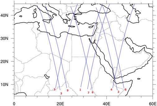
FIGURE 1. Model domain and CALIPSO paths during the dust event.
Satisfactory dust storm forecasts over the MENA region require realistic representation of the local geographic conditions (terrain, soil, landuse, vegetation) and the atmospheric circulations both at regional and local scales. Clearly, a fully coupled dust/aerosol and dynamic atmospheric model that both resolves the geographic and dust conditions and simulates and predicts dust and dynamic weather is ideal. In this regard, the fully coupled Weather Research and Forecasting with chemistry (WRF-Chem) model (Grell et al., 2005; Fast et al., 2006; Peckham et al., 2011) is a promising candidate. The WRF-Chem model has been previously used to investigate dust storms and dust interactions with atmospheric thermodynamics and radiation in many regions of the world and has shown satisfactory performance (e.g., Zhao et al., 2010; Smoydzin et al., 2012; Kalenderski et al., 2013; Kumar et al., 2014; Zhang et al., 2015; Flaounas et al., 2017; Parajuli et al., 2020b). However, a detailed evaluation of the model performance over the MENA region is needed for dust forecasting applications.
Proper simulation of dust uptake and transport requires accurate meteorological conditions. For that end we have coupled the WRF-Chem model with the WRF-based Real-Time Four-Dimensional Data Assimilation and forecasting (RTFDDA) system developed at the Research Applications Laboratory (RAL) of the National Center for Atmospheric Research (NCAR). The core of the RTFDDA system is a data assimilation component that continuously assimilates meteorological observations as they become available, thereby producing model-observation integrated 4D datasets that both define the current atmospheric conditions and serve as the initial conditions for subsequent model forecasts (Liu et al., 2006; Huang et al., 2018). This approach effectively alleviates the spin-up issue in short-term weather forecasting as continuous assimilation provides initial conditions that are consistent with both the dynamic equations in the model and the atmospheric states provided by the observations.
In this study we evaluate the skill of the coupled WRF-Chem-RTFDDA model in reproducing a dust storm event that covered extended areas of the MENA region. The event, which took place between 14 March and 18 March 2016, was due to a low-level cold frontal system and an upper-level low-pressure system initially located over the Western Mediterranean that moved slowly east-southeastward. Strong southwesterly winds both at the low level and the upper level developed along the southeast side of the low-pressure system, giving rise to significant dust emissions. We investigate the forecast skill as a function of forecast lead times and as a function of the RTFDDA cycling strategy. Satellite observations provided by the Spinning Enhanced Visible and Infrared Imager (SEVIRI) on the European Meteorological Satellite (EUMETSAT), the Moderate Resolution Imaging Spectroradiometer (MODIS) and the Cloud-Aerosol Lidar and Infrared Pathfinder Satellite Observations (CALIPSO) missions as well as the Copernicus Atmosphere Monitoring Service (CAMS) aerosol re-analysis (Bozzo et al., 2017) are used for verification.
WRF-Chem is a fully coupled meteorology-chemistry-aerosol model that simulates simultaneously the emission, transport, deposition, mixing and chemical transformation of trace gasses and aerosols, as well as their interactions with meteorology (Grell et al., 2005). Cloud chemistry, aerosol-cloud interactions, and their feedback processes were also incorporated into the WRF-Chem model (Fast et al., 2006; Chapman et al., 2009). In this study, the Air Force Weather Agency (AFWA) (Jones et al., 2012) dust emission scheme with “dust only” chemistry option is used for the application purpose of completing and issuing the forecasts in a timely manner. This scheme computes dust emission as a function of wind speed, soil moisture, and particle size, and uses the same dust source strength function as in Ginoux et al. (2001), to represent the availability of loose erodible soil material (LeGrand et al., 2019). The dust source strength function is a topography-based function (Ginoux et al., 2001)
representing the probability value assigned to cell i for having accumulated sediments at elevation
The main physical mechanisms of dust lifting are wind erosion beyond the threshold friction velocity, the saltation bombardment and the disintegration of the aggregates. The threshold friction velocity of wind erosion is the velocity at which dust particles can be lifted from the surface directly by wind shear forces. The saltation bombardment occurs when sand particles or aggregates strike the surface, causing localized impacts that are often strong enough to overcome the binding forces acting on the dust particles, resulting in significant dust emission (Gillette, 1981; Kok et al., 2012; Scanza et al., 2015). During severe wind erosion, dust layers attached to sand grains in sandy soils or as aggregates in soils with high clay content initially difficult to release by low wind erosion can disintegrate causing increased emission of dust, and this process is called the disintegration of aggregates.
The dust emission flux in the scheme is distributed into five different size bins with an effective particle radius of 0.1–1.0, 1.0–1.8, 1.8–3.0, 3.0–6.0, and 6.0–10 μm, respectively. The emission within each bin is injected to the lowest model level, and the subsequent dispersion and transport are computed by the chemical module in conjunction with the meteorological fields.
The WRF-based RTFDDA (WRF-RTFDDA) relies on the Newtonian-relaxation data assimilation approach to create mesoscale analyses or reanalyses that combine observations with model fields (Liu et al., 2008a). The assimilation of observations using RTFDDA has been proved to improve the mesoscale flow simulations (Liu et al., 2008b). In the Newtonian relaxation approach, data assimilation (nudging) terms are added to the model prognostic equations. These nudging terms force the model solution at each grid point to approach point observations or gridded analyses of observations, proportionate to the assimilation increment (i.e., the difference between the modeled field and the observed field). This data assimilation approach is computationally efficient and it allows a continuous rather than intermittent assimilation of observations. Since the full model dynamics is part of the data assimilation system its analyses contain all locally forced mesoscale features. The implementation of Newtonian relaxation in the present modelling system forces the model solution toward point observations (Stauffer and Seaman, 1994) rather than toward a gridded analysis of them. This choice is based on the fact that mesoscale observations are in general not uniformly distributed in space, which makes objective analysis difficult. Each observation is assimilated at its observed time and location, with suitable space and time weights. The model dynamics spread the information in time and space, in particular in areas void of observations. A quality-control procedure is applied to the observations as described in Liu et al. (2004). A common finding in several studies that used the Newtonian relaxation (Stauffer et al., 1991; Stauffer and Seaman, 1994; Seaman et al., 1995) was that nudging toward observations of mesoscale flow was more successful than toward analyses. Hahmann et al. (2010) has shown the improvement in the simulated flow over our area of interest when the Newtonian-relaxation assimilation of observations was implemented.
The simulations were run with 9 km horizontal resolution and 57 vertical levels. The model domain can be seen in Figure 1. The surface erodibility map in shown in the Supplementary Figure S1.
The physical schemes used in the present work are as follows. For microphysics, longwave radiation and shortwave radiation we used WSM6 (Hong and Lim, 2006), RRTM (Mlawer et al., 1997) and Goddard (Chou et al., 2001), respectively. WSM6 is a single-moment scheme that prognoses the mass mixing ratio of 6 water species: water vapour, cloud water, rainwater, cloud ice, snow and graupel. RRTM uses preset tables to describe longwave radiation processes in relation to water vapor, ozone, carbon dioxide, and trace gasses. In the Goddard scheme, the solar spectrum is divided into eleven spectral bands (seven in the ultraviolet, UV; one in the visible or photosynthetic active region, PAR; and three in the near-infrared, near-IR). Noah LSM (Tewari et al., 2004) and MM5 similarity scheme (Beljaars, 1994) were used for Land Surface and Surface Layer physics, respectively. The Noah LSM has one canopy layer and one snow layer, and has the following prognostic variables: soil moisture and soil temperature in the soil layers, canopy moisture, snow height, and surface and ground runoff accumulation. Evapotranspiration is handled by using soil and vegetation types. The vegetation characteristics of each grid of the model are represented by the dominant vegetation type in that grid. The MM5 similarity scheme uses stability functions from Dyer and Hicks (1970), Paulson (1970) and Webb (1970) to compute surface exchange coefficients for heat, moisture and momentum. Four stability categories, stable, mechanically induced turbulence, unstable (forced convection) and unstable (free convection) following Zhang and Anthes (1982) are considered to compute the correction terms. This scheme has been modified recently by Jiménez et al. (2012) to be applicable for various stability conditions. A convective velocity following Beljaars (1994) is used to enhance surface fluxes of heat and moisture. No thermal roughness length parameterization is included. Over the water surface, the Charnock relation is used to compute the roughness length from the friction velocity. YSU (Hong et al., 2006) was used for boundary layer physics. The YSU scheme is a first order, non-local scheme with an explicit entrainment layer and a parabolic K-profile in an unstable mixed layer.
The simulations were conducted from 06 UTC March 13 till 18 UTC 18 March 2016 with 2 “cold starts” (CSs). In our case a CS is defined as the beginning of the continuous data assimilation and dust emissions. Free forecast (FF) runs were launched every 6 h (without data assimilation) out to 48 h, and we refer to them as FF cycles. We used the National Center for Environmental Prediction (NCEP) Global Analysis and Forecasts System (GFS) output at a horizontal resolution of 0.5° × 0.5° as initial and lateral boundary conditions. The first continuous data assimilation period (P1, following the first CS, CS1) started at 06 UTC March 13 and ended at 18 UTC March 16, with 14 FF cycles being launched every 6 h; while the second period (P2, following the second CS, CS2) started at 00 UTC March 16 and ended at 18 UTC March 18 and 12 FF cycles were launched during the period. The purpose for dividing the entire simulation length into two periods with two CSs was to reduce model errors that tend to grow with simulation time. There was a time overlap between the two data assimilation periods (4 FF cycles were launched for each period during the overlap time) that would enable us to examine the model FF simulations in terms of the distance from CS and in terms of FF lead time simultaneously. Table 1 summarizes the two data assimilation periods and FF runs. Observations were continuously assimilated after every CS as described in Section 3.2. Observations from several platforms were assimilated and these included surface, upper air and aircraft observations of wind, temperature, humidity and pressure as summarized in Supplementary Table S1 in the Supplementary Material. Since there was no assimilation of dust (either from global models or observations) there was no dust in the model atmosphere at the time of CS. Therefore, the nomenclature “cold start” refers in our case to the beginning of the dust processes as well.
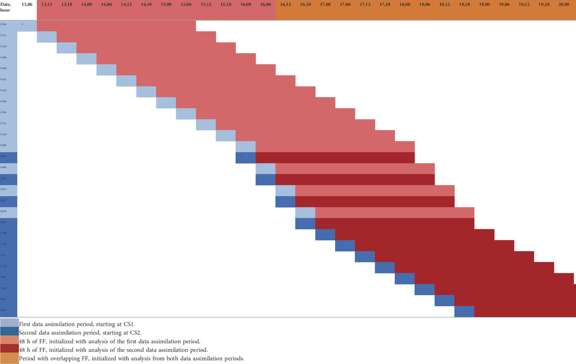
TABLE 1. Summary of WRF-Chem-RTFDDA runs. Pairs of numbers in first column and row indicate dates in March 2016 (from 13 to 18) and UTC time in 6-h intervals (from 00 to 18). Beginning of first continuous data assimilation period (P1) is indicated as one on the light-blue cell corresponding to 06 UTC 13 March 2016 (first cold start, CS1). Light-blue cells indicate 6-h intervals of continuous data assimilation following CS1 during P1. Light-red cells indicate 48-h free forecast (FF) initialized with analysis obtained at the end of each 6-h interval of continuous data assimilation during P1. Similar numbering and color rules but using dark-red and dark-blue are used for the second continuous data assimilation period, P2, starting on 00 UTC 16 March 2016 (second cold start, CS2). Colors in the first row indicate periods of time for which FF were initialized with analysis obtained during P1 (light-red), FF initialized with analysis obtained during P2 (dark-red) and FF initialized with analysis obtained during P1 and during P2 (brown). Bold values in the first column refer to FF during the second data assimilation period associated and following CS2.
Table 1: Summary of WRF-Chem-RTFDDA runs. Pairs of numbers in first column and row indicate dates in March 2016 (from 13 to 18) and UTC time in 6-h intervals (from 00 to 18). The beginning of first continuous data assimilation period (P1) is indicated as one on the light-blue cell corresponding to 06 UTC 13 March 2016 (first cold start, CS1). Light-blue cells indicate 6-h intervals of continuous data assimilation following CS1 during P1. Light-red cells indicate 48-h free forecast (FF) initialized with analysis obtained at the end of each 6-h interval of continuous data assimilation during P1. Similar numbering and color rules but using dark-red and dark-blue are used for the second continuous data assimilation period, P2, starting at 00 UTC 16 March 2016 (second cold start, CS2). Colors in the first row indicate periods of time for which FF were initialized with analysis obtained during P1 (light-red), FF initialized with analysis obtained during P2 (dark-red) and FF initialized with analysis obtained during P1 and during P2 (brown). Bold values in the first column refer to FF during the second data assimilation period associated and following CS2.
Multispectral products are generated from the Spinning Enhanced Visible and Infrared Imager (SEVIRI) instrument on the geostationary Meteosat Second Generation (MSG) satellite and operationally implemented to address a number of forecast challenges for both daytime and nighttime applications (https://sds-was.aemet.es/news/meteosat-rgb-dust-product-for-the-middle-east). It is referred to as “RGB Imagery” or “RGB Products,” as brightness temperatures or paired band differences are used to set the red, green, and blue intensities of each pixel in the final image, resulting in a false-color composite (EUMETSAT, 2009). The EUMETSAT MSG dust product is derived from infrared channels of SEVIRI. It is designed to monitor the evolution of dust storms over deserts during both day and night. The RGB combination exploits the difference in emissivity of dust and desert surfaces (Lensky and Rosenfeld, 2008). In addition, during daytime, it exploits the temperature difference between the hot desert surface and the cooler dust cloud. The RGB composite is produced using the following MSG IR channels: IR12.0-IR10.8 (on red), IR10.8-IR8.7 (on green); and IR10.8 (on blue). Dust appears pink or magenta in this RGB combination. Dry land has the appearance from pale blue (daytime) to pale green (nighttime). Thick, high-level clouds have red-brown tones and thin high-level clouds appear very dark (nearly black). The sampling frequency is 15 min and the spatial resolution at nadir is 3 km.
Comparison to the Meteosat images could reveal the spatial evaluation of modeled total lifted dust, but does not tell much about the vertical distribution of dust. It is the total dust along the column that the Meteosat images show.
The Cloud-Aerosol Lidar and Infrared Pathfinder Satellite Observations (CALIPSO), part of the NASA Afternoon Constellation (A-Train, https://www-calipso.larc.nasa.gov/about/atrain.php), has a 98°-inclination orbit and is placed in a 705 km sun-synchronous polar orbit, which provides global coverage between 82°N and 82°S with a local afternoon equatorial crossing time of about 1:30 p.m. CALIPSO carries a cloud-aerosol lidar with orthogonal polarization (CALIOP). CALIOP utilizes three receiver channels: one measuring the 1,064 nm backscatter intensity and two other channels measuring orthogonally polarized components of the 532 nm backscattered signal. The receiver telescope is 1 m in diameter. The vertical resolution of the products is 30 m between 0 and 8 km (above mean sea level—AMSL) and 60 m between 8 and 20 km AMSL. The satellite samples the atmosphere along narrow paths (1 km width) which repeat every 16 days. Figure 1 shows the model domain and the CALIPSO paths during the dust event and the dates and hours of the paths are listed in Supplementary Table S2 in the Supplementary Material.
The comparison between the model FF simulations and CALIOP observations is based on the extinction coefficient measured by the lidar (CALIPSO level-2 product, measurements that do not refer to dust are excluded) and that calculated from the modeled dust concentrationof the five dust bins assuming uniform spherical dust particles and the size distribution and density characteristics of the five dust bins used by the AFWA emissions scheme (Section 2.1. Jones et al., 2012). The extinction coefficient is directly proportional to dust concentrations.
The MODIS instrument aboard the Terra and Aqua satellites monitors the entire surface of the Earth every 1–2 days. The many data products derived from the MODIS measurements describe features of the land, oceans and the atmosphere including the ambient aerosol optical thickness (AOD). The MODIS Level-2 atmospheric aerosol product (MOD04_L2) provides full global coverage of aerosol properties based on the Dark Target (DT) and Deep Blue (DB) algorithms (e.g., Levy et al., 2013; Sayer et al., 2014; Sayer et al., 2015). The DT algorithm is applied over ocean and dark land (e.g., vegetation), while the DB algorithm is applied over the entire land areas including both vegetated regions and bright surfaces. Over the vegetated regions, the DB algorithm makes use of NDVI (Normalized Difference Vegetation Index) and a precalculated surface reflectance database to derive the aerosol properties. The latest collection (C6) of the MOD04_L2 products include an estimate on the aerosol retrieval uncertainty to assist with error analyses as well as a best estimate dataset containing the aerosol optical thickness with quality assurance flag. The datasets are provided on a 10 km × 10 km pixel scale in Hierarchical Data Format (HDF-EOS). Each MOD04_L2 product file covers a 5-min time interval.
In this work, all of the MOD04_L2 product files that fall within the area of 4°N—50°N, 10°W—70°E during March 13—18 March 2016 were downloaded from the MODIS data portal (https://ladsweb.modaps.eosdis.nasa.gov/missions-and-measurements/products/MOD04_L2/). These product files were first regridded onto the model grid and then combined together for the same hour (10:30 for the morning pass and 13:30 for the afternoon pass) for the same day. We compared the 10:30 files with the 13:30 files for the same day and we did not notice appreciable differences between the two. The reason might be that 10:30 and 13:30 are not that far away from each other. For the analysis, we will use the 10:30 MODIS AOD data to compare with the modelled data at 11:00 (since the model output is hourly).
In order to evaluate the model skill in reproducing the atmospheric conditions needed for the dust emissions, a comparison between the FF and the observed surface wind speeds was made. Root mean square error (RMSE), bias and correlation were calculated at station locations for 10 m winds above the ground level. Supplementary Figure S2 in the Supplementary Material shows the distributions of the stations used in the verification: the choice of the stations was based on the availability of the observations and whether or not they were located in the areas prone to dust. Verification metrics were hourly and were calculated over all stations. The station observations used for verification were assimilated into the model during the continuous assimilation periods. However, we evaluate here the skill of the FF that did not assimilate the station observations. This is a well-established procedure in model verification.
CAMS aerosol re-analysis, spanning from 2003 to 2021, includes both the two-dimensional and three-dimensional atmospheric parameters at a spatial resolution of about 80 km and a 3-hourly output frequency. CAMS re-analysis uses a 4DVAR (4-dimensional Variational) data assimilation technique and has 60 pressure levels from the surface to 0.1 hPa. CAMS re-analysis has been shown to represent aerosol climatology over many parts of the world satisfactorily (Bozzo et al., 2017).
Figures 2A–C presents the RMSE, bias and correlation calculated over the surface stations, respectively, valid at the hours from all the WRF-Chem FF runs. In general, the RMSE is the lowest (1.5–2 m/s, Figure 2A) and the correlation the highest (0.7–0.8, Figure 2C) at +1 h lead time, except for the FF runs immediately following the CSs. Between +3 and 12 h lead time, the RMSE stays in the range of 2–2.5 m/s and the correlation in the range of 0.6–0.7 but the RMSE increases and the correlation decreases with progressively longer lead time. This behavior indicates that after the first cycle following the CS the system tends to be spun-up already and thereafter error grows with lead time. In addition, the FF runs immediately following the CS2 (hereafter referred to as P2) show lower RMSE than those following CS1 (hereafter referred to as P1) by ∼0.5 m/s on average, in a similar magnitude to the difference in the mean wind speeds between the two periods (i.e., 4.6 m/s for P1 vs. 4.1 m/s for P2 leading to a difference of 0.5 m/s). The bias lies between -1 and 1 m/s for most of the runs (Figure 2B).
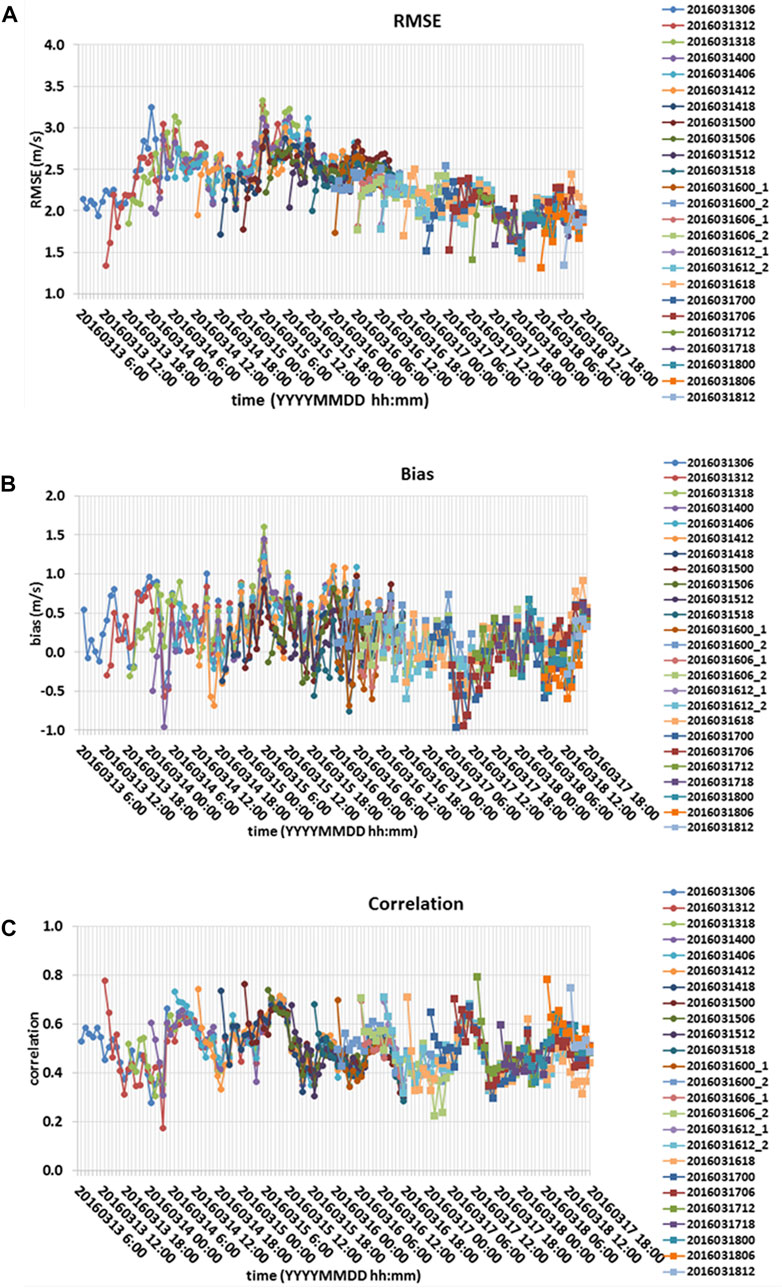
FIGURE 2. (A) RMSE, (B) Bias, and (C) Correlation of 10-m wind speed (m/s) calculated over all the stations. Filled circles and filled squares represent free forecast cycles following the first and second cold starts, respectively. The X axis lists the dates and hours of the start of the free forecast cycles. Different colors represent different free forecasts cycles.
Dust simulations from all of the FF runs were compared to the Meteosat images. The FF runs succeeded in reproducing the main features of the spatial distribution of the dust, most of the “hot spots” locations (areas where dust loads are significant), and the timings of the occurrence of the dust storms revealed in the Meteosat images, but several differences in dust behavior exist between different FF runs. As mentioned earlier, due to the 6-hourly cycling in our assimilation and forecasting system with 48-h free forecasts, there are overlaps of various lengths amongst the successive cycles. Thus, by comparing the forecasts that are valid at the same hours but with different lead time, we could gain an understanding of the model performance dependence on forecast lead time and on time distance from the CS.
Figures 3, 4 present selected maps of dust (panel b–total dust, panel c–emitted dust) constructed based on the FF run outputs that are valid at the same hours from either the same cycles or the different cycles but with different lead time, together with the Meteosat images. The valid times of the Meteosat images, the forecast lead time and the time distance from the CS are all indicated at the top of the respective images. In the comparison we focused on specific geographic locations where dust loads were significant (hot spots) and evaluated the overall distribution of the dust in the studied region, too.
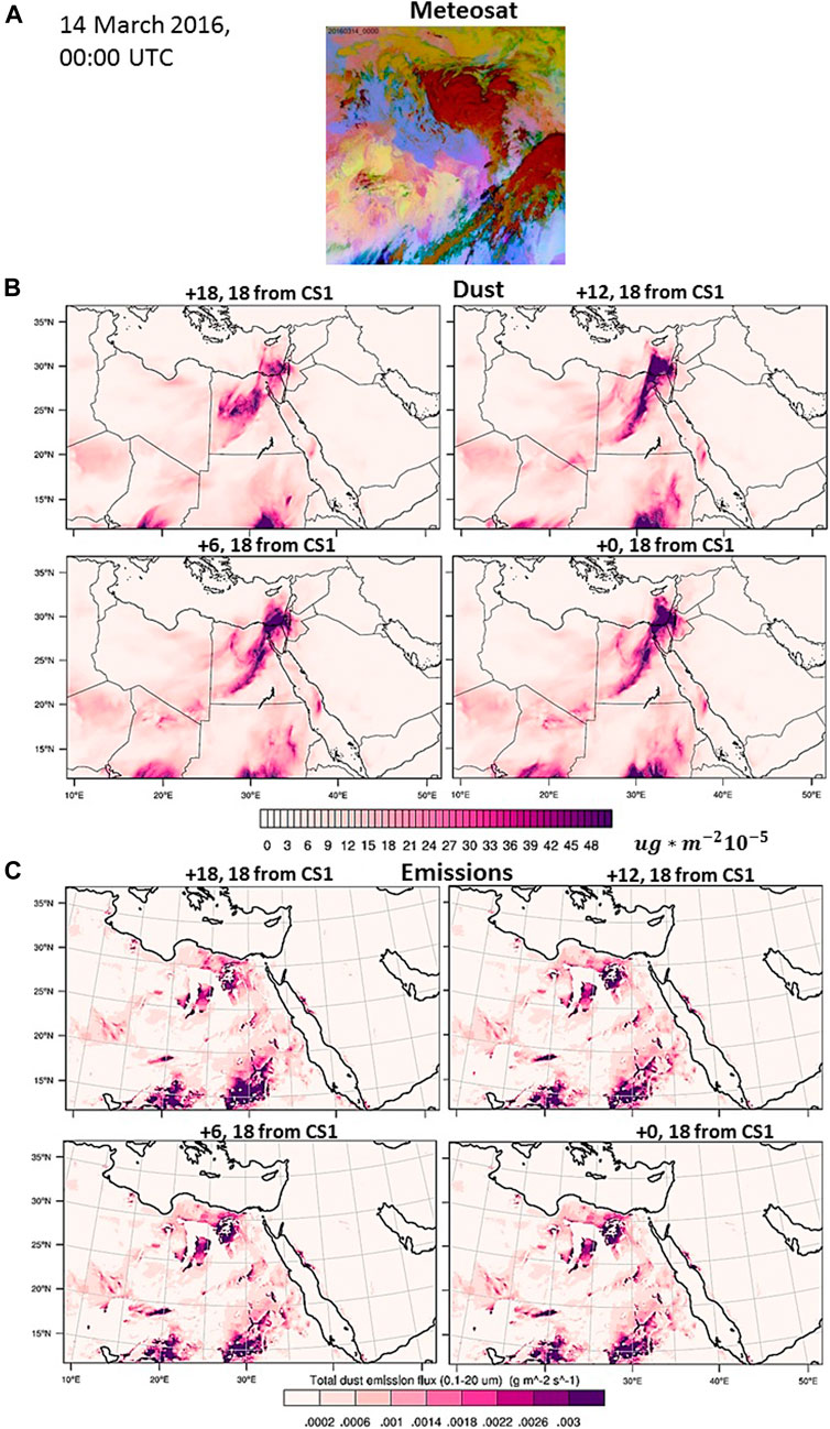
FIGURE 3. Comparison of the modeled total dust and emitted dust concentrations against the Meteosat measurements valid at 00 UTC 14 March 2016: (A) Meteosat image, (B) total dust (ug *m−210–5), (C) emitted dust (gm−2s−1). The valid time, forecast lead time and time distance from the CS (CS1 or CS2 representing the first or the second CS) are shown at the top of each panel.
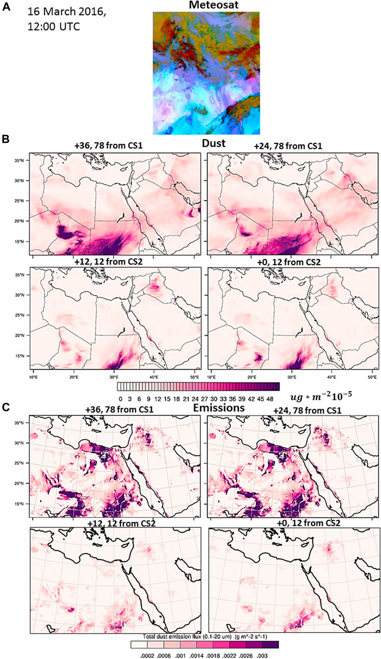
FIGURE 4. Same as Figure 3 but valid at 12 UTC 16 March 2016.
An example of different cycles within the same CS is presented in Figure 3, valid at 00 UTC March 14. The FF lead times ranged from 00 to +18 h, at a 6-hourly interval, and the time distance from the CS span from 0 to +18 h. The areas of interest are Egypt, Israel and their coasts. Two features can be noticed in Figure 3B 1) the simulated dust is more severe at longer time distance from the CS but shorter lead time; and 2) the spatial spread of the simulated dust increases with lead time as seen for example over the Eastern Mediterranean. It appears that the most significant difference between different cycles but valid at the same hours is in their spatial dust distribution. For the FF simulations with the shortest lead time, the dust is limited to the area from where it is lifted but for longer lead times the dust tends to be transported and dispersed away from the source area, similar to what the Meteosat images display. Maps of the emitted dust (Figure 3C) show very little differences between the simulations. Therefore, as far as dust emissions are concerned they are not sensitive to the forecast lead times at least in this analysis when the time distances from the CS range from 0 to 18 h. On the other hand, dust transport and dispersion appear to be the dominating factors in determining the differences between the FF runs of different lead times. We further discuss these points in Section 4.
Figure 4 presents a comparison of the FF simulations valid at 12 UTC 16 March, with different lead times and from different CSs. The FF lead times span from 00 to +36 h, at a 12-hourly interval, and the time distance from the CS ranged from +42 to +54 h for the first CS, and from 00 to +12 for the second CS. It can be seen that longer time distance from the CS and longer lead times produce much larger and more broadly dispersed dust concentrations than those with shorter time distance from the CS and shorter lead times (Figure 4B). Also, the FF run with 24-h lead time predicts more dust lifted over Iraq than the other lead times, better resembling what the Meteosat image indicates (Figure 4A). Contrary to Figure 3C, dust emissions in Figure 4C exhibit significant differences amongst the simulations: much larger and broader dust emissions correspond to longer time distance from the CS and longer lead times. This may indicate that when the time distance from the CS goes beyond a certain time period, e.g., +42 h in this case (as opposed to only +18 h in Figure 3C) significant differences in emitted dust can be obtained which would further affect the overall total dust distribution in the domain.
While comparisons with the Meteosat images could provide an indication of the model performance in resolving the dust horizontal spatial distribution, comparisons with the CALIPSO profiles could shed light on the model performance in resolving the dust vertical distribution. As done in Section 3.2, we evaluated the FF forecasts as a function of lead time and as function of the time distance from the CS.
Vertical cross sections of the extinction coefficients from CALIPSO and from the FF run outputs with different lead times and different time distance from the same cold start CS1 along CALIPSO Path #6 (see Figure 1) are presented in Figure 5. All cross sections are valid at 1130 UTC March 16 and extend from the surface to 6 km AMSL. White color in the CALIPSO cross-section panel denotes missing values while purple color represents values that did not pass quality check. Note that the extinction coefficient is directly proportional to dust concentrations in the dust dominated areas.
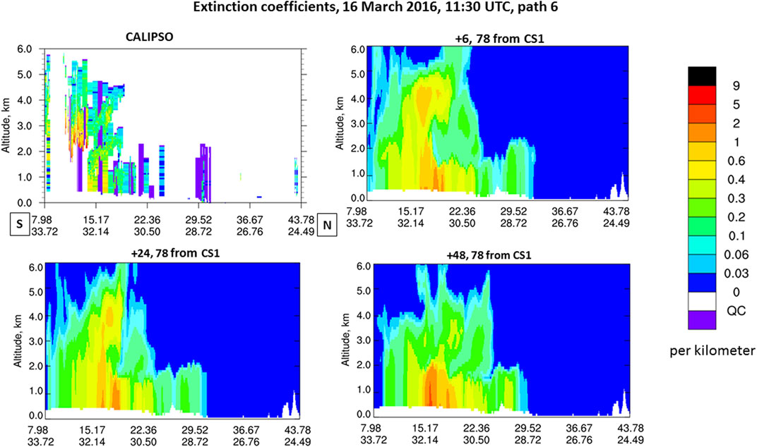
FIGURE 5. Vertical cross sections of CALIPSO and modeled extinction coefficients along CALIPSO Path #6 valid at 1130 UTC March 16. The modeled extinction coefficients in the different panels correspond to FF with different lead times and time distances from the same cold start CS1.
CALIPSO reveals moderate extinction coefficients between 14–17⁰N from the ground up to 2 km AMSL and large extinction coefficients between 11–14⁰N from ∼2 km up to ∼3.5 km AMSL. For the latter, we will not be able to know for sure if dust also existed below 2 km AMSL as the lidar might not be able to penetrate through these low layers when significant dust presented above them.
The modeled extinction coefficients are broadly consistent with what CALIPSO shows (Figure 5) in that elevated extinction coefficients are seen between 8–30⁰N, with large extinction coefficients generally identified between 14–17⁰N. However, in terms of the 11–14⁰N region, longer lead times of +36 h and +48 h appear to underestimate the observed large extinction coefficients from ∼2 to ∼3.5 km AMSL while the shorter lead times of +6 h and +18 h appear to overestimate the observed moderate extinction coefficients from ∼3.5 to ∼5.5 km AMSL. In terms of the 14–17⁰N region, all five forecast lead times correspond to large extinction coefficients although longer lead times of +36 h and +48 h appear to overestimate the observed extinction coefficients while shorter lead times of +6 h to +24 h appear to underestimate the vertical extend of the observed extinction coefficients. All things considered, it seems that the FF runs with +24 h and +48 h lead times are the closest to what CALIPSO reveals.
Along CALIPSO Path #7 (see Figure 1 for the location), significantly large values of extinction coefficients can be seen in CALIPSO in the 11.5–14⁰N band up to 2 km AMSL and then moderate extinction coefficients between 2 and 4 km AMSL (Figure 6). In addition, elevated extinction coefficients can be seen stretching from 21⁰N to 29⁰N up to 1.5 km AMSL. Again, the modeled extinction coefficients are broadly consistent with what CALIPSO shows (Figure 6) but there are clear differences between the simulations and the observations. In the 11.5–14⁰N band, overprediction of the observed extinction coefficients in the low levels tends to get improved with lead time; however, for longer lead times the model progressively simulates smaller extinction coefficients in the middle levels when compared to the observations. In the 21–29⁰N band, longer lead times lead to enhanced (reduced) extinction coefficients in the low (middle) levels. Based on this analysis, it also appears that the FF runs with +24 h and +48 h lead times match best to what CALIPS reveals.
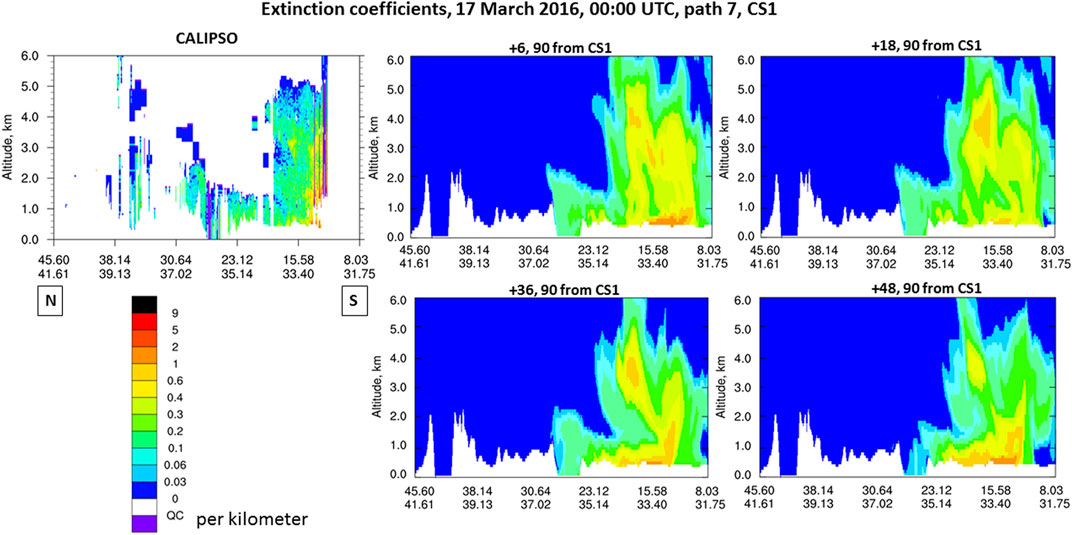
FIGURE 6. Same as Figure 5 except along CALIPSO Path #7 and valid at 00 UTC March 17.
Figure 7 extends Figure 6 by including some FF runs that were launched following CS2. This time, same +24 h lead time but different time distance from the CS leads to quite different distribution of extinction coefficients (Figure 7). With +6 h and +24 h lead times and +24 h time distance from the CS2, the modeled extinction coefficients are much more confined in both horizontal and vertical extent when compared to the FF runs that launched following CS1. It is possible that the weaker mean winds in P2 when compared to P1 may be partially responsible for the limited spatial spread of dust in P2.
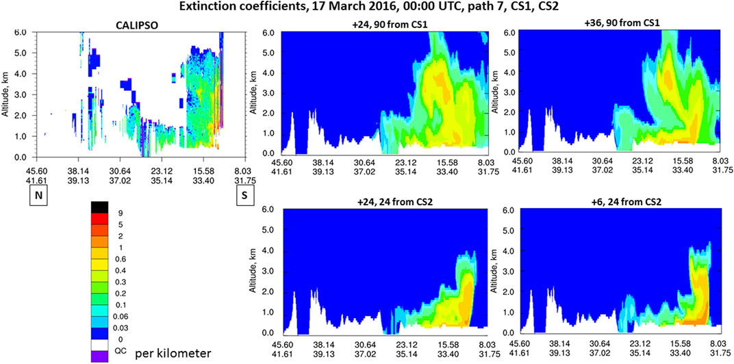
FIGURE 7. Same as Figure 6, except that some of the FF runs were initialized following CS2.
Along CALIPSO Path #8 (see Figure 1 for the location), large extinction coefficients can be seen from about 1 to 1.5 km AMSL with moderate extinction coefficients from 1.5 to 2.5 km AMSL between 17.5–27.5⁰N, and large to moderate extinction coefficients from near surface to 2.5 km AMSL around 34⁰N in the observations (Figure 8). The FF runs that were launched following the CS1 simulate elevated extinction coefficients between 1 and 2.5 km AMSL for 17.5–27.5⁰N and near surface to 2.5 km AMSL around 34⁰N but with reduced magnitude when compared to the observations. Also, these FF runs extend the elevated extinction coefficients from 2.5 km to beyond 6.0 km AMSL for 17.5–27.5⁰N, in clear contrast to the observations (Figure 8). The FF runs that were launched following the CS2 simulate some elevated extinction coefficients in those two areas but the magnitude and spatial extent are much lower than what CALIPSO reveals.
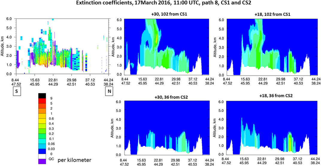
FIGURE 8. Same as Figure 7 except along CALIPSO path #8.
This section presents the CALIPSO mean extinction coefficients and mean RMSE, bias and correlation between CALIPSO measured and modeled extinction coefficients along each path and within the vertical layers of 0–6 km, 0–2 km, 2–4 km, and 4–6 km AMSL.
For the majority of the paths, dust is mostly concentrated below 2 km AMSL (Figure 9A). The exception is for Path #3, #6, and #9 for which the largest extinction coefficients (>0.3) amongst the layers are noted for the 2–4 km AMSL layer (for Path #3 the 4–6 km AMSL layer also shows significantly more dust than the 0–2 km AMSL layer; Figure 9A), and for these paths, RMSE tends to be the largest (Figure 9B) with clear model underestimation of dust load (Figure 9C) and generally reduced correlation (Figure 9D). Also, with the exception for Path #5, the FF runs following the CS usually underestimates dust load (Figure 9C). The extinction coefficient, RMSE and bias are usually the lowest for the 4–6 km AMSL layer when compared to the other layers but correlation is not necessarily the lowest for the 4–6 km AMSL layer. The differences in RMSE are larger between different paths than between the FF runs following different CSs.
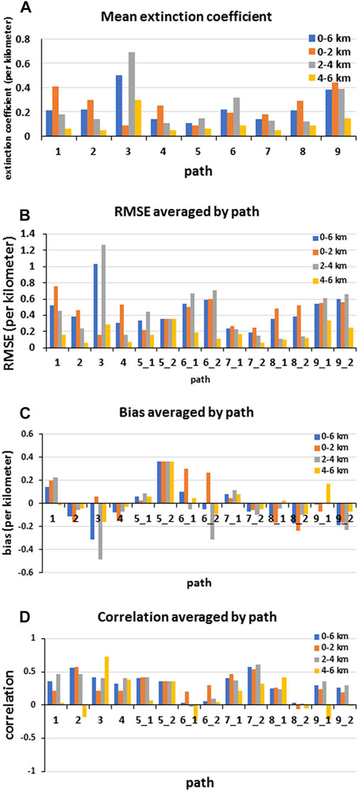
FIGURE 9. Mean extinction coefficient measured by CALIPSO (A), RMSE (B), bias (C) and correlation (D) between CALIPSO measured and modeled extinction coefficient along each path and within different vertical layers. The second digit following the path number refers to the cold start: “1” for CS1 and “2” for CS2.
In addition, we calculated RMSE, bias and correction of the extinction coefficients over all the paths as a function of forecast lead time (Figure 10). RMSE is the lowest and correlation is the highest for the +24 h lead time, while bias stays almost the same for all lead times (Figure 10). The +24 h lead time also displays the smallest differences between the maximum and the minimum values in RMSE, bias and correlation. On average, the model underestimates the dust load at all lead times. Compared to Figure 9, it can be inferred that the differences in RMSE, bias and correlations between different lead times are much lower than those between different paths or between different CSs.
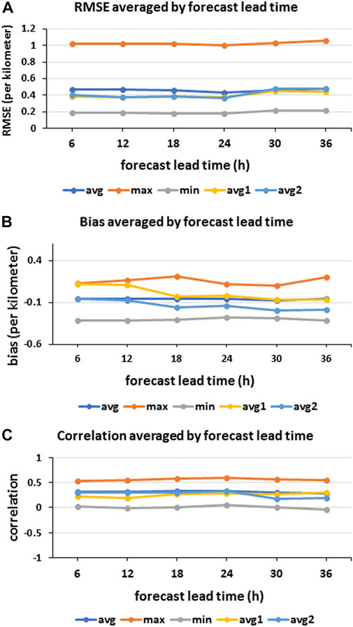
FIGURE 10. RMSE (A), bias (B), and correlation (C) between modeled and CALIPSO measured extinction coefficients for the 0–6 km AMSL layer over all the paths as a function of forecast lead time.
Here we present AOD comparisons between MODIS retrievals and WRF-Chem FF as well as between CAMS aerosol re-analysis and WRF-Chem FF.
We analyzed all FF forecasts close to the MODIS observation times and present here representative examples. Looking at all FF we notice that there is apparent similarity in AOD structure and evolutions between MODIS/CAMS and WRF-Chem FF in that wherever and whenever there is an indication of elevated AOD in MODIS/CAMS; all or a majority of the FF runs also show elevated AOD accordingly although there are discrepancies in terms of areal extent and magnitude (Figure 11). It should be noted that while WRF-Chem tends to overestimate MODIS AOD in some areas, CAMS noticeably underestimates MODIS AOD in all places. WRF-Chem succeeds in reproducing high MODIS AOD values at localized spots where CAMS fails. Due to the partial spatial coverage of the MODIS AOD observations, we calculated false alarms rates (FARs) with respect to CAMS using AOD = 0.4 as a threshold for the occurrence of a dust storm. FARs range from 0.03 to 0.26, with many of them staying below 0.15, indicating satisfactory performance of the modeling system. Interestingly, similar FARs are revealed for the FF runs from the same CS regardless of the FF lead time, confirming that the time distance from the CS plays a more important role in determining the model forecast skill. It appears that the model simulations, especially those from the CS1, consistently overestimates MODIS measured or CAMS analyzed AOD (Figure 11).
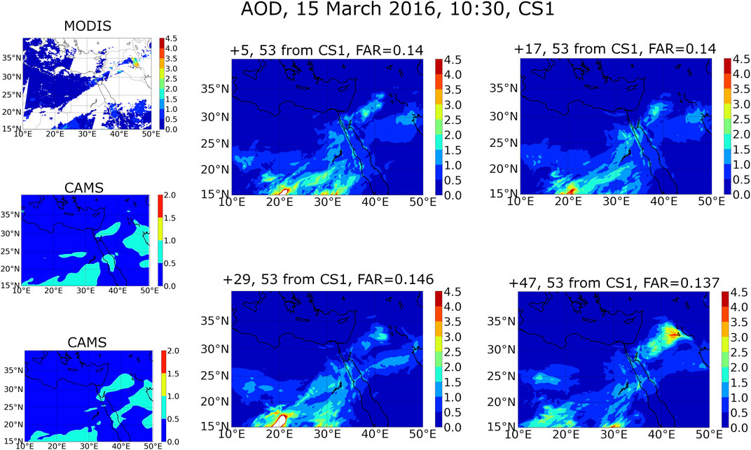
FIGURE 11. Comparison of modeled, MODIS and CAMS AOD values for 10:30 UTC (11:00 UTC for model) of 15 March 2016. The forecast lead time, time distance from the CS1 and false alarm rates are shown at the top of each modeled panel.
The FARs for different FF lead times and different CSs (Figure 12) further illustrate the satisfactory model performance as the FARs never go beyond 0.26 for CS1 and 0.15 for CS2. Similar to what was mentioned above, the FARs for the same cold start show more or less the same values independent of the forecast lead time. Also, the FARs corresponding to CS1 are larger than those of CS2 due to the overestimation of AOD by the FF runs from CS1.
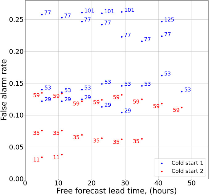
FIGURE 12. False alarm rates as a function of free forecast lead time and time distance from cold starts. Numbers next to the points represent hours from the cold start.
As stated in Section 2.3, the simulations neither included assimilation of dust observations nor used a global dust model for dust initial and lateral boundary conditions. The simulated dust is a result of WRF-Chem emissions and transport. The comparison to Meteosat images shows that the free forecasts that were close to the cold starts and had short lead times tended to underestimate dust concentrations, especially for the cases when the observed dust was transported from a different area. For instance, following the examples presented in Section 3.2 we can roughly estimate the required lead times and time distances from the cold starts for satisfactory dust forecasts. Our comparison to Meteosat suggests that +18 h after the cold starts are enough. The sensitivity to free forecast lead time is weaker as differences between free forecasts with different lead times for the valid time are rather small.
Furthermore, comparison of WRF-Chem AOD to MODIS and CAMS AOD values supports the insights achieved from the comparison to Meteosat images. The spatial distribution of AOD values indicating a dust storm (AOD >0.4) in WRF-Chem free forecasts overlaps with that from MODIS and CAMS to a large extent. The dependency of free forecasts skill on their lead times and distance from cold starts is similar to that observed in the comparison to Meteosat. However, comparison of AOD values enables a more quantitative assessment of WRF-Chem free forecasts. From the joint WRF-Chem, MODIS and CAMS AOD comparison we note that while CAMS systematically underpredicts AOD values with respect to MODIS, WRF-Chem succeeds in reproducing AOD values similar to those retrieved by CAMS in localized areas.
The vertical extent of the dust plume depends on the proximity to the cold starts and on the lead time of the forecasts. Free forecasts very close to the cold starts and with short lead times created dust plums that did not rise high enough. The free forecasts runs with +24 h lead times found to be the closest to the observed in terms of the spatial patterns and overall statistics. While we observe an overestimation in the modeled dust concentration at lower levels and an underestimation at higher levels, the total column dust concentration roughly matched what was measured by CALIPSO. Cases in which high concentration of dust was measured (extinction coefficient >0.3 per kilometer) showed the highest root mean squared errors between the simulations and the observations. From the vertical cross-sections and the dust maps we clearly see that dust concentration values above “hot spots” strongly depend on the dust emissions, while above other areas dust concentrations are dominated by transport and dispersion. False alarm rates range between 0.03 and 0.26 indicating quite satisfactory performance of the system as a warning system.
The results of our analysis show that dust forecasts produced by a mesoscale model in which simulated emissions are the only source of elevated dust (with no elevated dust in the initial conditions) may show different error growth patterns than those found in meteorological forecast variables (e.g., wind, temperature) following data assimilation. Our wind-speed verification against surface observations, as well as verification of WRF-RTFDDA against surface and upper observations found in literature (e.g., Wyszogrodzki et al., 2013; Pan et al., 2021) illustrates this fact. In Figure 2 and in Pan et al. (2021) error growth starts at the very few hours after free forecast initialization following data assimilation, and may saturate or continue to grow with free forecast lead time. This is expected as errors in the initial conditions propagate into the forecasts and the positive impact of assimilation reduces as the atmospheric state evolves. However, dust concentrations need to build up as dust is emitted from surface prone areas. Therefore, in the absence of dust in the initial conditions, error in forecast dust concentrations decreases as model emissions produce elevated dust and transports it. Since we run continuous assimilation of meteorological variables at the same time that dust is emitted and transported, the overall dust concentrations are a result of the emitted and transported dust during the continuous assimilation period up to the initialization of the free forecasts (time distance from cold start), as well as a result of the emitted and transported dust during the free forecasts period (free forecast lead time). Therefore, the time thresholds indicated above, +18 from cold start and +24 h of free forecasts provide guidelines on dust spin-up times within the WRF-Chem-RTFDDA system as used in this work. Dust free forecasts produced before these spin-up times are prone to larger errors and forecasters should avoid using them. Our analysis still shows lesser impact of free forecasts lead times on their skill than that of the period of time since the cold start. This fact demonstrates that once dust is spun-up the free forecasts are reliable independent of their lead time, therefore, even those approaching the end of the free forecasting horizon can be trustably used by forecasters. Continuous data assimilation of up to +18 h should be performed before launching free forecasts with the present WRF-Chem-RTFDDA system.
The WRF-Chem-RTFDDA forecasts presented in this work can be improved in several ways, the simplest of which may include: 1) using a more realistic database for the potential for dust emissions within the WRF-Chem model. Several databases of high-resolution dust potential calibrated to various areas have been developed in recent years and are available to the scientific community (e.g., Parajuli et al., 2019); 2) using initial and lateral boundary dynamic conditions from global models with finer resolution such as the ECMWF IFS (Owens and Hewson (2018); and 3) using initial and lateral boundary chemical conditions from global dust models such as CAMS (Morcrette et al., 2009).
In this work we evaluated the performance of the WRF-Chem-RTFDDA modeling system in the forecasts of dust storms over the MENA region at 9-km resolution. The system continuously assimilated conventional meteorological observations. No global dust model was used for initialization and no dust observations were assimilated into the model. We note that meteorological observations are sparse in large areas of the MENA region. These limitations present a significant challenge to the forecasting system. We analyzed the skill of the WRF-Chem-RTFDDA analyses and forecasts in reproducing the horizontal spatial distribution of the dust storm by comparing them with the Meteosat SEVIRI dust images and AOD retrieved by MODIS and analyzed by CAMS. The skill of the model in resolving the vertical dust distribution was assessed by comparing the modeled and CALIPSO measured extinction coefficients. The skill was analyzed as a function of free forecast lead time and as a function of the time distance from the cold starts, when continuous data assimilation and dust emissions were initiated with the aim of spinning-up the system. Statistical verification of the modeled extinction coefficients in terms of RMSE, bias and correction was conducted using the CALIPSO measured extinction coefficients. Our results show that WRF-Chem-RTFDDA reproduced the main features of the dust storms during the study period. In this modeling system, the time distance from the CS appears to play a more significant role in influencing the dust forecast skills than the free-forecast lead time. Since no external dust information was provided to the model, dust forecasts in this modeling system depended critically on dust emissions and spin-up by WRF-Chem. The vertical extent of the CALIPSO extinction coefficients were fairly well reproduced by the model once model emissions were spun-up. However, the modeled vertical distribution of the extinction coefficients showed more noticeable differences between different CALIPSO paths than the forecast lead times or the time distance from the CS. Differences in the modeled dust load over the “hot spots” were mainly a result of the intensity of the dust emissions. Differences away from the “hot spots” were a result of transport and dispersion of the emitted dust. The latter was especially evident over the sea. The vertical extent of the dust was primarily determined by the time distance to the CS. To the best of our knowledge this is the first study in which a comparison between the FF run output against three types of satellite observations (Meteosat, MODIS and CALIPSO), including objective verification scores, as a function of lead time and time distance to the CS is performed. Calculation of false alarms rates shows that the system can fairly be used as a warning tool. Our study shows the feasibility of dust forecasts over the MENA region using minimal input data.
The original contributions presented in the study are included in the article/Supplementary Material, further inquiries can be directed to the corresponding author.
All authors listed have made a substantial, direct, and intellectual contribution to the work and approved it for publication.
This research was supported in part by the PAZY Foundation of the Israel Atomic Energy Commission (Grant No. 122-2020). The National Center for Atmospheric Research is sponsored by the National Science Foundation.
The authors declare that the research was conducted in the absence of any commercial or financial relationships that could be construed as a potential conflict of interest.
All claims expressed in this article are solely those of the authors and do not necessarily represent those of their affiliated organizations, or those of the publisher, the editors and the reviewers. Any product that may be evaluated in this article, or claim that may be made by its manufacturer, is not guaranteed or endorsed by the publisher.
The Supplementary Material for this article can be found online at: https://www.frontiersin.org/articles/10.3389/fenvs.2022.981852/full#supplementary-material
Alharbi, B. H. (2009). Airborne dust in Saudi Arabia: Source areas, entrainment, simulation and composition. Ph.D. Thesis (Monash, Australia: Monash University), 345.
Beljaars, A. C. M. (1994). The parameterization of surface fluxes in large-scale models under free convection. Q. J. R. Meteorol. Soc. 121, 255–270.
Bou Karam, D., Flamant, C., Cuesta, J., Pelon, J., and Williams, E. (2010). Dust emission and transport associated with a Saharan depression: February 2007 case. J. Geophys. Res. 115, D00H27. doi:10.1029/2009JD012390
Bou Karam, D., Flamant, C., Knippertz, P., Reitebuch, O., Pelon, J., Chong, M., et al. (2008). Dust emissions over the sahel associated with the West african monsoon intertropical discontinuity region: A representative case-study. Q. J. R. Meteorol. Soc. 134, 621–634. doi:10.1002/qj.244
Bozzo, A., Remy, S., Benedetti, A., Flemming, J., Bechtold, P., Rodwell, M. J., et al. (2017). Implementation of a CAMS-based aerosol climatology in the IFSA. ECMWF Technical Memorandum 801, 33.
Bristow, C. S., HudsonEdwards, K. A., and Chappell, A. (2010). Fertilizing the amazon and equatorial atlantic with West African dust. Geophys. Res. Lett. 37, L14807. doi:10.1029/2010GL043486
Chapman, E. G., Gustafson, W. I., Easter, R. C., Barnard, J. C., Ghan, S. J., Pekour, M. S., et al. (2009). Coupling aerosol-cloud-radiative processes in the WRF-chem model: Investigating the radiative impact of elevated point sources. Atmos. Chem. Phys. 9, 945–964. doi:10.5194/acp-9-945-2009
Chauvin, F., Roehrig, R., and Lafore, J. P. (2010). Intraseasonal variability of the Saharan heat low and its link with midlatitudes. J. Clim. 23, 2544–2561. doi:10.1175/2010jcli3093.1
Chou, M.-D., Suarez, M. J., Liang, X.-Z., and Yan, M. M.-H. (2001). A thermal infrared radiation parameterization for atmospheric studies. NASA Tech. Memo. 56, 104606. Available at: http://ntrs.nasa.gov/search.jsp?R=20010072848 (Accessed August 1, 2014).
D’Almeida, G. A. (1986). A model for Saharan dust transport. J. Clim. Appl. Meteor. 25, 903–916. doi:10.1175/1520-0450(1986)025<0903:amfsdt>2.0.co;2
Dayan, U., Heffter, J., Miller, J., and Gutman, G. (1991). Dust intrusion events into the Mediterranean basin. J. Appl. Meteor. 30, 1185–1199. doi:10.1175/1520-0450(1991)030<1185:dieitm>2.0.co;2
Dyer, A. J., and Hicks, B. B. (1970). Flux-gradient relationships in the constant flux layer. Q. J. R. Meteorol. Soc. 96, 715–721. doi:10.1002/qj.49709641012
Engelstaedter, S., Tegen, I., and Washington, R. (2006). North African dust emissions and transport. Earth. Sci. Rev. 79, 73–100. doi:10.1016/j.earscirev.2006.06.004
Evan, A. T., Fiedler, S., Zhao, C., Menut, L., Schepanski, K., Flamant, C., et al. (2015). Derivation of an observation-based map of North African dust emission. Aeolian Res. 16, 153–162. doi:10.1016/j.aeolia.2015.01.001
Fast, J. D., Gustafson, W. I., Easter, R. C., Zaveri, R. A., Barnard, J. C., Chapman, E. G., et al. (2006). Evolution of ozone, particulates, and aerosol direct radiative forcing in the vicinity of Houston using a fully coupled meteorology-chemistry-aerosol model. J. Geophys. Res. 111, D21305. doi:10.1029/2005JD006721
Flaounas, E., Bastin, S., and Janicot, S. (2011). Regional climate modelling of the 2006 West African monsoon: Sensitivity to convection and planetary boundary layer parameterisation using WRF. Clim. Dyn. 36, 1083–1105. doi:10.1007/s00382-010-0785-3
Flaounas, E., Janicot, S., Bastin, S., Roca, R., and Mohino, E. (2012). The role of the Indian monsoon onset in the West african monsoon onset: Observations and AGCM nudged simulations. Clim. Dyn. 38, 965–983. doi:10.1007/s00382-011-1045-x
Flaounas, E., Kotroni, V., Lagouvardos, K., Kazadzis, S., Gkikas, A., and Hatzianastassiou, N. (2015). Cyclone contribution to dust transport over the Mediterranean region. Atmos. Sci. Lett. 16, 473–478. doi:10.1002/asl.584
Flaounas, E., Kotroni, V., Lagouvardos, K., Klose, M., Flamant, C., and Giannaros, T. M. (2017). Sensitivity of the WRF-chem (V3.6.1) model to different dust emission parametrisation: Assessment in the broader mediterranean region. Geosci. Model. Dev. 10, 2925–2945. doi:10.5194/gmd-10-2925-2017
Gazeaux, J., Flaounas, E., Naveau, P., and Hannart, A. (2011). Inferring change points and nonlinear trends in multivariate time series: Application to West African monsoon onset timings estimation. J. Geophys. Res. 116, D05101. doi:10.1029/2010JD014723
Gillette, D. A. (1981). Production of dust that may be carried great distances. Geol. Soc. Am. Special Pap. Geol. Soc. Am. 1981, 11–26. doi:10.1130/SPE186-p11
Ginoux, P., Chin, M., Tegen, I., Prospero, J. M., Holben, B., Dubovik, O., et al. (2001). Sources and distributions of dust aerosols simulated with the GOCART model. J. Geophys. Res. 106 (D17), 20255–20273. doi:10.1029/2000jd000053
Goudie, A. S. (2009). Dust storms: Recent developments. J. Environ. Manag. 90, 89–94. doi:10.1016/j.jenvman.2008.07.007
Grell, G. A., Peckham, S. E., Schmitz, R., McKeen, S. A., Frost, G., Skamarock, W. C., et al. (2005). Fully coupled “online” chemistry within the WRF model. Atmos. Environ. X. 39, 6957–6975. doi:10.1016/j.atmosenv.2005.04.027
Hahmann, A. N., Rostkier-Edelstein, D., Warner, T. T., Liu, Y., Vandenberghe, F., and Swerdlin, S. P. (2008). Toward a climate downscaling for the Eastern Mediterranean at high-resolution. Adv. Geosci. 12, 159–164. doi:10.5194/adgeo-12-159-2008
Hahmann, A. N., Rostkier-Edelstein, D., Warner, T. T., Vandenberghe, F., Liu, Y., Babarsky, R., et al. (2010). A reanalysis system for the generation of mesoscale climatographies. J. Appl. Meteorol. Climatol. 490 (5), 954–972. doi:10.1175/2009JAMC2351.1
Hong, S., and Lim, J. (2006). The WRF single-moment 6-class microphysics scheme (WSM6). J. Korean Meteor. Soc. 42, 129–151.
Hong, S., Noh, Y., and Dudhia, J. (2006). A new vertical diffusion package with an explicit treatment of entrainment processes. Mon. Weather Rev. 134, 2318–2341. doi:10.1175/mwr3199.1
Huang, Y., Liu, Y., Xu, M., Liu, Y., Pan, L., Wang, H., et al. (2018). Forecasting severe convective storms with WRF-based RTFDDA radar data assimilation in Guangdong, China. Atmos. Res. 209, 131–143. doi:10.1016/j.atmosres.2018.03.010
Huneeus, N., Schulz, M., Balkanski, Y., Griesfeller, J., Prospero, J., Kinne, S., et al. (2011). Global dust model intercomparison in AeroCom phase I. Atmos. Chem. Phys. 11, 7781–7816. doi:10.5194/acp11-7781-2011
Jiménez, P. A., Dudhia, J., González-Rouco, J. F., Navarro, J., Montávez, J. P., and García-Bustamante, E. (2012). A revised scheme for the WRF surface layer formulation. Mon. Weather Rev. 140, 898–918. doi:10.1175/mwr-d-11-00056.1
Jones, S. L., Adams-Selin, R., Hunt, E. D., Creighton, G. A., and Cetola, J. D. (2012). Update on modifications to WRF-CHEM GOCART for fine-scale dust forecasting at AFWA. Chicago: AGU Fall Meeting Abstracts.
Kalenderski, S., Stenchikov, G., and Zhao, C. (2013). Modeling a typical winter-time dust event over the arabian peninsula and the red sea. Atmos. Chem. Phys. 13, 1999–2014. doi:10.5194/acp-13-1999-2013
Kaufman, Y. J., Tanre, D., and Boucher, O. (2002). A satellite view of aerosols in the climate system. Nature 419 (6903), 215–223. doi:10.1038/nature01091
Kaufman, Y. J., Tanrè, D., and Boucher, O. (2002). A satellite view of aerosols in the climate system. Nature 419, 215–223. doi:10.1038/nature01091
Kaufman, Y., Koren, I., Remer, L., Tanre, D., Ginoux, P., and Fan, S. (2005). Dust transport and deposition observed from the TerraModerate resolution imaging spectroradiometer (MODIS) spacecraft over the atlantic ocean. J. Geophys. Res. 110, D10S12. doi:10.1029/2003JD004436
Klein, C., Heinzeller, D., Bliefernicht, J., and Kunstmann, H. (2015). Variability of West African monsoon patterns generated by a WRF multi-physics ensemble. Clim. Dyn. 45, 2733–2755. doi:10.1007/s00382-015-2505-5
Klose, M., Shao, Y., Karremann, M. K., and Fink, A. H. (2010). Sahel dust zone and synoptic background. Geophys. Res. Lett. 37, L09802. doi:10.1029/2010GL042816
Klose, M., and Shao, Y. (2013). Large-eddy simulation of turbulent dust emission. Aeolian Res. 8, 49–58. doi:10.1016/j.aeolia.2012.10.010
Knippertz, P., and Todd, M. C. (2012). Mineral dust aerosols over the Sahara: Meteorological controls on emission and transport and implications for modeling. Rev. Geophys. 50, RG1007. doi:10.1029/2011RG000362
Kok, J. F., Parteli, E. J. R., Michaels, T. I., and Karam, D. B. (2012). The physics of wind-blown sand and dust. Rep. Prog. Phys. 75, 106901. doi:10.1088/0034-4885/75/10/106901
Kumar, R., Barth, M. C., Pfister, G. G., Naja, M., and Brasseur, G. P. (2014). WRF-chem simulations of a typical pre-monsoon dust storm in northern India: Influences on aerosol optical properties and radiation budget. Atmos. Chem. Phys. 14, 2431–2446. doi:10.5194/acp-14-2431-2014
LeGrand, S. L., Polashenski, C., Letcher, T. W., Creighton, G. A., Peckham, S. E., and Cetola, J. D. (2019). The AFWA dust emission scheme for the GOCART aerosol model in WRF-Chem v3.8.1. 12. Geosci. Model. Dev. 2019, 131–166.
Lelieveld, J., Evans, J. S., Fnais, M., Giannadaki, D., and Pozzer, A. (2015). The contribution of outdoor air pollution sources to premature mortality on a global scale. Nature 525, 367–371. doi:10.1038/nature15371
Lensky, I. M., and Rosenfeld, D. (2008). Clouds-aerosols-precipitation satellite analysis tool (CAPSAT). Atmos. Chem. Phys. 8, 6739–6753. doi:10.5194/acp-8-6739-2008
Levy, R. C., Mattoo, S., Munchak, L. A., Remer, L. A., Sayer, A. M., Patadia, F., et al. (2013). The Collection 6 MODIS aerosol products over land and ocean. Atmos. Meas. Tech. 6, 2989–3034. doi:10.5194/amt-6-2989-2013
Liu, Y., Chen, F., Warner, T., and Basara, J. (2006). Verification of a mesoscale data-assimilation and forecasting system for the Oklahoma City area during the joint urban 2003 field project. J. Appl. Meteorol. Climatol. 45 (7), 912–929. doi:10.1175/jam2383.1
Liu, Y., Vandenberghe, F., Low-Nam, S., Warner, T. T., and Swerdlin, S. (2004). “Observation-quality estimation and its application in the NCAR/ATEC real-time FDDA and forecast (RTFDDA) system,” in Preprints, 20th Conf. on Weather Analysis and Forecasting and 16th Conf. on Numerical Weather Prediction (Seattle, WA: Amer. Meteor. Soc.), J1.7.
Liu, Y., Warner, T. T., Astling, E. G., Bowers, J. F., Davis, C. A., Halvorson, S. F., et al. (2008b). The operational mesogamma-scale Analysis and forecast system of the U.S. Army test and evaluation command. Part II: Interrange comparison of the accuracy of model analyses and forecasts. J. Appl. Meteorology Climatol. 47, 1093–1104. doi:10.1175/2007jamc1654.1
Liu, Y., Warner, T. T., Bowers, J. F., Carson, L. P., Chen, F., Clough, C. A., et al. (2008a). The operational mesogamma-scale analysis and forecast system of the U.S. Army Test and Evaluation Command. Part I: Overview of the modeling system, the forecast products, and how the products are used. J. Appl. Meteorology Climatol. 47, 1077–1092. doi:10.1175/2007jamc1653.1
Miller, S. D., Kuciauskas, A. P., Liu, M., Ji, Q., Reid, J. S., Breed, D. W., et al. (2008). Haboob dust storms of the southern Arabian Peninsula. J. Geophys. Res. 113, D01202. doi:10.1029/2007JD008550
Mlawer, E. J., Taubman, S. J., Brown, P. D., Iacono, M. J., and CLough, S. A. (1997). Radiative transfer for inhomogeneous atmospheres: RRTM, a validated correlated-k model for the longwave. J. Geophys. Res. 102D, 16663–16682. doi:10.1029/97jd00237
Mohalfi, S., Bedi, H. S., Krishnamurti, T. N., and Cocke, S. D. (1998). Impact of shortwave radiative effects of dust aerosols on the summer season heat low over Saudi Arabia. Mon. Weather Rev. 126, 3153–3168. doi:10.1175/1520-0493(1998)126<3153:iosreo>2.0.co;2
Morcrette, J. J., Boucher, O., Jones, L., Salmond, D., Bechtold, P., Beljaars, A., et al. (2009). Aerosol analysis and forecast in the European centre for medium-range weather forecasts integrated forecast system: Forward modeling. J. Geophys. Res. 114, D06206. doi:10.1029/2008JD011235
Moulin, C., Lambert, C. E., Dulac, F., and Dayan, U. (1997). Control of atmospheric export of dust from North Africa by the North atlantic oscillation. Nature 387, 691–694. doi:10.1038/42679
Notaro, M. F. A., Fadda, E., and Bakhrjy, F. (2013). Trajectory analysis of Saudi Arabian dust storms. J. Geophys. Res. Atmos. 118, 6028–6043. doi:10.1002/jgrd.50346
Pan, L., Liu, Y., Roux, G., Cheng, W., Liu, Y., Hu, J., et al. (2021). Seasonal variation of the surface wind forecast performance of the high-resolution WRF-RTFDDA system over China. Atmos. Res. 259, 105673. doi:10.1016/j.atmosres.2021.105673
Parajuli, S. P., Stenchikov, G. L., Ukhov, A., and Kim, H. (2019). Dust emission modeling using a new high-resolution dust source function in WRF-Chem with implications for air quality. JGR. Atmos. 124 (10), 10109–10133. doi:10.1029/2019JD030248
Parajuli, S. P., Stenchikov, G. L., Ukhov, A., Shevchenko, I., Dubovik, O., and Lopatin, A. (2020b). Aerosol vertical distribution and interactions with land/sea breezes over the eastern coast of the Red Sea from lidar data and high-resolution WRF-Chem simulations. Atmos. Chem. Phys. 20, 16089–16116. doi:10.5194/acp-20-16089-2020
Parajuli, S. P., Stenchikov, G. L., Ukhov, A., Shevchenko, I., Dubovik, O., and Lopatin, A. (2020a). Interaction of dust aerosols with land/sea breezes over the eastern coast of the red sea from LIDAR data and high-resolution WRF-chem simulations. Atmos. Chem. Phys. Discuss.
Paulson, C. A. (1970). The mathematical representation of wind speed and temperature profiles in the unstable atmospheric surface layer. J. Appl. Meteor. 9, 857–861. doi:10.1175/1520-0450(1970)009<0857:tmrows>2.0.co;2
Peckham, S. E., Grell, G. A., McKeen, S. A., Bath, M., Pfiser, G., Wiedinmyer, C., et al. (2011). WRF/Chem version 3.3 user's guide, 96.
Prospero, J. M., Collard, F. X., Molinié, J., and Jeannot, A. (2014). Characterizing the annual cycle of African dust transport to the Caribbean Basin and South America and its impact on the environment and air quality. Glob. Biogeochem. Cycles 28, 757–773. doi:10.1002/2013GB004802
Prospero, J. M., Ginoux, P., Torres, O., Nicholson, S. E., and Gill, T. E. (2002). Environmental characterization of global sources of atmospheric soil dust identified with the Nimbus 7 total ozone mapping spectrometer (TOMS) absorbing aerosol product. Rev. Geophys. 40, 2-1–2-31. doi:10.1029/2000RG000095
Prospero, J. M. (1996). “Saharan dust transport over the North atlantic ocean and mediterranean: An overview,” in The impact of desert dust across the mediterranean. Editors S. Guerzoni, R. Chester, and Kluwer (Dordrecht, Netherlands: Springer Netherlands), 133–152.
Sayer, A. M., Hsu, N. C., Bettenhausen, C., Jeong, M.-J., and Meister, G. (2015). Effect of MODIS Terra radiometric calibration improvements on collection 6 Deep blue aerosol products: Validation and terra/aqua consistency. J. Geophys. Res. Atmos. 120. doi:10.1002/2015JD023878
Sayer, A. M., Munchak, L. A., Hsu, N. C., Levy, R. C., Bettenhausen, C., and Jeong, M.-J. (2014). MODIS Collection 6 aerosol products: Comparison between Aqua's e-Deep Blue, Dark Target, and "merged" data sets, and usage recommendations. J. Geophys. Res. Atmos. 119, 13965–13989. doi:10.1002/2014JD022453
Scanza, R. A., Mahowald, N., Ghan, S., Zender, C. S., Kok, J. F., Liu, X., et al. (2015). Modeling dust as component minerals in the community atmosphere model: Development of framework and impact on radiative forcing. Atmos. Chem. Phys. 15, 537–561. doi:10.5194/acp-15-537-2015
Seaman, N. L., Stauffer, D. R., and Lario-Gibbs, A. M. (1995). A multiscale four-dimensional data assimilation system applied in the San-Joaquin Valley during SARMAP. Part I: Modeling design and basic performance characteristics. J. Appl. Meteor. 34 (8), 1739–1761. doi:10.1175/1520-0450(1995)034<1739:AMFDDA>2.0.CO;2
Smoydzin, L., Teller, A., Tost, H., Fnais, M., and Lelieveld, J. (2012). Impact of mineral dust on cloud formation in a Saharan outflow region. Atmos. Chem. Phys. 12, 11383–11393. doi:10.5194/acp-12-11383-2012
Stauffer, D. R., Seaman, N. L., and Binkowski, F. S. (1991). Use of four-dimensional data assimilation in a limited-area mesoscale model. Part 2. Effects of data assimilation within the planetary boundary-layer. Mon. Wea. Rev. 119 (3), 734–754. doi:10.1175/1520-0493(1991)119<0734:UOFDDA>2.0.CO;2
Stauffer, D. R., and Seaman, N. L. (1994). Multiscale four-dimensional data assimilation. J. Appl. Meteor. 33, 416–434. doi:10.1175/1520-0450(1994)033<0416:mfdda>2.0.co;2
Sultan, B., Janicot, S., and Drobinski, P. (2007). Characterization of the diurnal cycle of the West African monsoon around the monsoon onset. J. Clim. 20, 4014–4032. doi:10.1175/jcli4218.1
Tanaka, T. Y., and Chiba, M. (2006). A numerical study of the contributions of dust source regions to the global dust budget. Glob. Planet. Change 52, 88–104. doi:10.1016/j.gloplacha.2006.02.002
Tegen, I. (2003). Modeling the mineral dust aerosol cycle in the climate system. Quat. Sci. Rev. 22 (18–19), 1821–1834. doi:10.1016/s0277-3791(03)00163-x
Tegen, I., and Fung, I. (1994). Modeling of mineral dust in the atmosphere: Sources, transport, and optical thickness. J. Geophys. Res. 99 (D11), 22897. doi:10.1029/94jd01928
Tewari, M., Chen, F., Wang, W., Dudhia, J., LeMone, M., Mitchell, K. E., et al. (2004). “Implementation and verification of the unified Noah land surface model in the WRF model,” in 20th Conference on Weather Analysis and Forecasting/16th Conference on Numerical Weather Prediction, Seattle, Washington, 11-15 January, 2004.
Tindale, N. W., and Pease, P. P. (1999). Aerosols over the Arabian Sea: Atmospheric transport pathways and concentrations of dust and sea salt. Deep Sea Res. Part II Top. Stud. Oceanogr. 46, 1577–1595. doi:10.1016/s0967-0645(99)00036-3
Tsvetsinskaya, E. A., Schaaf, C. B., Gao, F., Strahler, A. H., Dickinson, R. E., Zeng, X., et al. (2002). Relating MODIS-derived surface albedo to soils and rock types over Northern Africa and the Arabian peninsula. Geophys. Res. Lett. 29, 67-1–67-4. doi:10.1029/2001GL014096
Tyrlis, E., Škerlak, B., Sprenger, M., Wernli, H., Zittis, G., and Lelieveld, J. (2014). On the linkage between the Asian summer monsoon and tropopause fold activity over the eastern Mediterranean and the Middle East. J. Geophys. Res. Atmos. 119, 3202–3221. doi:10.1002/2013JD021113
Wang, W., Evan, A. T., Flamant, C., and Lavaysse, C. (2015). On the decadal scale correlation between african dust and sahel rainfall: The role of saharan heat low-forced winds. Sci. Adv. 1, e1500646. doi:10.1126/sciadv.1500646
Washington, R., Todd, M. C., Lizcano, G., Tegen, I., Flamant, C., Koren, I., et al. (2006). Links between topography, wind, deflation, lakes and dust: The case of the Bodélé Depression, Chad. Geophys. Res. Lett. 33, L09401. doi:10.1029/2006GL025827
Webb, E. K. (1970). Profile relationships: The log-linear range, and extension to strong stability. Q. J. R. Meteorol. Soc. 96, 67–90. doi:10.1002/qj.49709640708
World Health Organisation (WHO) (2014). Burden of disease from air pollution. Available at: http://www.who.int/phe/health_topics/outdoorair/databases/FINAL_HAP_AAP_BoD_24March2014.pdf?ua=1.
Wyszogrodzki, A. A., Liu, Y., Jacobs, N., Childs, P., Zhang, Y., Roux, G., et al. (2013). Analysis of the surface temperature and wind forecast errors of the NCAR-AirDat operational CONUS 4-km WRF forecasting system. Meteorol. Atmos. Phys. 122, 125–143. doi:10.1007/s00703-013-0281-5
Zhang, D. L., and Anthes, R. A. (1982). A high-resolution model of the planetary boundary layer—Sensitivity tests and comparisons with SESAME-79 data. J. Appl. Meteor. 21, 1594–1609. doi:10.1175/1520-0450(1982)021<1594:ahrmot>2.0.co;2
Zhang, Y., Liu, Y., Kucera, P. A., Alharbi, B. H., Pan, L., and Ghulam, A. (2015). Dust modeling over Saudi Arabia using WRF-Chem: March 2009 severe dust case. Atmos. Environ. 119, 118–130. doi:10.1016/j.atmosenv.2015.08.032
Zhao, C., Liu, X., Leung, L. R., Johnson, B., McFarlane, S. A., Gustafson, W. I., et al. (2010). The spatial distribution of mineral dust and its shortwave radiative forcing over North Africa: Modeling sensitivities to dust emissions and aerosol size treatments. Atmos. Chem. Phys. 10, 8821–8838. doi:10.5194/acp-10-8821-2010
Keywords: WRF-Chem, RTFDDA, dust forecasts, MENA, in-situ observations, MENA, remote sensing products
Citation: Rostkier-Edelstein D, Kunin P, Sheu R-S, Gelman A, Yunker A, Roux G, Pietrkowski A and Zhang Y (2022) Evaluation of WRF-Chem-RTFDDA dust forecasts over the MENA region using in-situ and remote-sensing observations. Front. Environ. Sci. 10:981852. doi: 10.3389/fenvs.2022.981852
Received: 29 June 2022; Accepted: 29 August 2022;
Published: 11 October 2022.
Edited by:
Sagar Parajuli, King Abdullah University of Science and Technology, Saudi ArabiaReviewed by:
Rama Krishna Karumuri, King Abdullah University of Science and Technology, Saudi ArabiaCopyright © 2022 Rostkier-Edelstein, Kunin, Sheu, Gelman, Yunker, Roux, Pietrkowski and Zhang. This is an open-access article distributed under the terms of the Creative Commons Attribution License (CC BY). The use, distribution or reproduction in other forums is permitted, provided the original author(s) and the copyright owner(s) are credited and that the original publication in this journal is cited, in accordance with accepted academic practice. No use, distribution or reproduction is permitted which does not comply with these terms.
*Correspondence: Dorita Rostkier-Edelstein, ZHJvc3RraWVyQHlhaG9vLmNvbQ==
Disclaimer: All claims expressed in this article are solely those of the authors and do not necessarily represent those of their affiliated organizations, or those of the publisher, the editors and the reviewers. Any product that may be evaluated in this article or claim that may be made by its manufacturer is not guaranteed or endorsed by the publisher.
Research integrity at Frontiers
Learn more about the work of our research integrity team to safeguard the quality of each article we publish.