Computational fluid dynamics simulation of rough bed open channels using openFOAM

With increased flood risk due to climate change, population expansion and urbanisation; robust waterway design and management are critical. One common type of waterway used to gather and transport ground water is the open channel. Most simulations do not account for the physical roughness of the bed, instead using a roughness coefficient. This means that only the turbulent energy content can be modelled whilst physical turbulent eddies and vortices cannot. Furthermore, many past studies assume the free surface is a rigid lid. This could affect the way that turbulent structures near the free surface behave. Computational Fluid Dynamics simulation of an open channel with a rough bed and rigid lid are conducted using OpenFOAM. Results show good correlation with experimental tests. It can be visually observed that turbulent structures generated from the rough bed do interact with the free surface and thus a rigid lid is perhaps not a great approximation. This is supported by an apparent decrease in the Reynolds shear stress from the free surface and 30% of the flow depth immediately beneath.

1 Introduction

Shallow open channels are one of the most commonly used geometries for water transport; examples being man-made aqueducts, canals and other natural waterways with a water-air interface. Many of these waterways form key water infrastructure to prevent flooding and deliver clean water. It has been shown experimentally that the patterns and behaviour of the water surface are correlated with some underlying flow properties (e.g. flow velocity) as well as physical properties (e.g. bed roughness) (see e.g. Lamb, 1993; Savelsberg and van de Water, 2008; Horoshenkov et al., 2013). Horoshenkov et al. (2013) looked at spatial correlation of water surface waves generated in shallow water flows over a gravel bed without appreciable bed forms. It was shown that a mathematical function could be used to correlate the spatial correlation radius, lag and characteristic period to the depth-averaged flow velocity, the vertical velocity profile, bed roughness, hydraulic roughness and the flow Reynolds number. These were explored further experimentally by Nichols et al. (2013) who proposed further relationships, however more research needs to be conducted to develop more generalised knowledge of the mechanisms behind these relationships. Muraro et al. (2021) provides a good review of all the current state of research. If a reliable correlation can be established, it may be possible to use the latest innovations in 3D scanning (e.g. LIDAR) and digital signal processing to remotely assess the water surface and deduce key performance characteristics of the waterway such as water carrying capacity (see e.g. Horoshenkov et al., 2016; Nichols and Rubinato, 2016; Nichols et al., 2020). This could be critical in identifying early warning signs of flooding such as increasing depth of flow. Given the unpredictability of climate change, this could become a vital tool.

Much of the existing literature on open channel Computational Fluid Dynamics (CFD) simulations use a smooth bed with some wall function to estimate the amount of turbulent energy that would be in the flow if a real material with physical roughness were used (Tan et al., 2015). Whilst this can represent the average energies, it cannot replicate transient effects such as the generation of vortex structures at the bed (Komori et al., 1989), their movement within the flow, interaction with other turbulent structures (Kline et al., 1967; Adrian et al., 2000) and ultimately, their breakdown and eventual dissipation (Grass, 1971; Roy et al., 2004). Part of the reason is due to the existence of a roughness boundary layer near the bed which is heavily dependent on the bed geometry. The variability of the bed geometries makes artificial modelling of the roughness boundary layer a challenge (Jimenez, 2004). Using a physically rough bed instead of wall functions would resolve this however, this requires a very high quality mesh which imposes a very high computational cost. The computational power that was available in the past was low (Moore’s law dictates the number of transistors on a microchip doubles about every two years) so computational power 20 years ago is almost a thousand times less than modern capabilities (see e.g. Burg and Ausubel, 2021)).

Some numerical studies of open channel flow with physical bed roughness do exist. Singh et al. (2007) performed Direct Numerical Simulation (DNS) on a hexagonal closed packed bed of spheres to study the nature of the flow near the bed. Good agreement with experimental results are seen for the mean velocity, turbulence intensities, and Reynolds stress. A Large Eddy Simulation (LES) was initially run for around 30T (where T = d/u_τ is the large-eddy turnover time) to obtain a fully developed turbulent field. This was then mapped onto a DNS simulation. The depth of flow has been taken as four times the diameter of the spheres. This was achieved using a simulation domain of $4\sqrt{3}d\times 4d\times d$ (streamwise × spanwise × depth) although the actual values of the sphere diameters was never revealed. Furthermore, a rigid lid free surface was used and claimed to be appropriate due to small surface deformations.

Another study by Stoesser and Rodi (2007) used spheres of 22 mm in diameter in a hexagonal closed packed bed formation to simulate flow over a rough bed using LES code MGLET. The results showed excellent agreement with the measured data of Detert (2005) and conformity with the log law for rough walls. However, it should be noted that the experimental data was unpublished. The depth of flow was h = 94 mm relative to the top of the spheres. The domain was 5h in streamwise, 2h in spanwise and 1h in vertical directions. In total, 46 million mesh points were used. The grid spacing in terms of wall units were Δx⁺ = 5 in the streamwise direction and Δz⁺ = 7 in the spanwise direction. In the vertical direction the grid spacing was kept at a constant value of Δy⁺ = 2.5 at the bed and then stretched towards free surface. Periodic boundary conditions were applied in the streamwise and spanwise directions with a constant pressure gradient driving the flow. The free surface was not discussed at all.

Bomminayuni and Stoesser (2011) also repeated a similar LES simulation but using hemi-spheres. They state that a 2πH × πH × H domain size for smooth bed flows is commonly accepted. A common theme is that periodic boundary conditions are used in the streamwise direction to reduce the size of the computational domain. Once again, the free surface was not modelled with the claim that a rigid lid was sufficient.

Alfonsi et al. (2019) used LES to simulate flow over rocks with a median size of 70 mm. OpenFOAM was used with Wall-Adapting-Local-Eddies (WALE) wall modelling. WALE is a sub-grid scale closure model first proposed by Nicoud and Ducros (1999) as a new sub-grid model for complex geometries. The model is able to simulate near wall eddy viscosity and accounts for the effects of the strain and the rotation in the smallest resolved turbulent fluctuations. This was also used by Adrian et al. (2000) in OpenFOAM. Unlike the previous studies, Alfonsi et al. (2019) used the interFOAM approach to capture the free surface using a Volume of Fluid (VoF) method. Results were compared to ADV measurements of laboratory flows in terms of turbulence statistics and turbulent laws, showing a good agreement and demonstrating that OpenFOAM was able to simulate open channel flows with rough beds.

Table 1, 2 summarises some of the key studies discussed. It can be seen that whilst there are some advances in free surface modelling Kazemi et al. (2020), many studies claim a rigid lid is an appropriate simplification of the simulation (see e.g. Satoru et al., 1982; Borue et al., 1995; Nagaosa, 1999; Nagaosa and Handler, 2003). This is understandable as a significant number of cells are required to capture the free surface interface properly, especially if the surface fluctuations are small (Dao et al., 2018). Mesh also cannot be refined suddenly at the free surface and a gradual gradient is required which further increases mesh difficulty. However, few studies provide actual evidence that the turbulent structures which are generated from the rough bed are not affected by the rigid lid simplification. The aim of this paper is to investigate the effect of a rigid lid approximation on the flow. To achieve this, a rough bed simulation is designed. The next section uses the information gathered during the literature review and presents the final setup of the CFD simulation.

TABLE 1

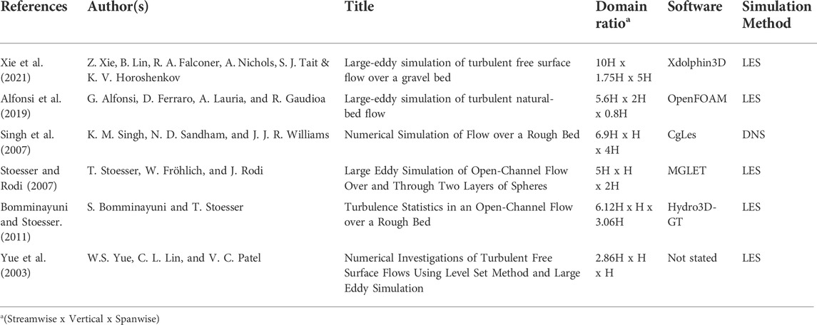
TABLE 1. Summary of rough bed simulations and domain ratio used.

TABLE 2

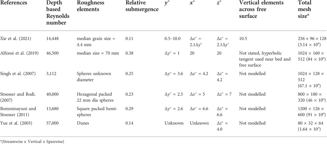
TABLE 2. Summary of rough bed simulations and CFD parameters.

2 Materials and methods

The simulation is split into two stages. The first stage uses a coarse mesh and a wider computational domain with RANS calculation to stabilise and obtain time averaged statistics comparable to the experimental results. The second stage takes these results and uses the MapFields utility in OpenFOAM to map them onto a finer mesh with a smaller computational domain. LES calculation with the Wall-Adapting-Local-Eddies (WALE) method is then used to develop transient turbulent effects for closer analysis.

The simulation uses a rigid lid to purposefully and artificially remove the effect of the free surface. This means that unlike in real life, the water surface is not allowed to fluctuate. It is anticipated that the turbulent structures which grow from the bed and propagate upwards will hit the surface and deform. This would suggest that without a flexible lid, the response of the structure to the free surface would be different (the analogy being a solid object landing on a trampoline vs. landing on concrete ground).

2.1 Validation against experimental tests

Experiments were conducted at the University of Sheffield’s water laboratory for validation of the CFD model. The tests were carried out using a 15 m long recirculating flume with a width of 500 mm. A full bed of spheres with a 24 mm diameter was used in a hexagonal close packing pattern.

Particle Imaging Velocimetry (PIV) techniques were applied 10 m from the upstream inlet to obtain a velocity field along the flume’s centerline. A flat laser light sheet illuminated the tracer particles in the measurement region from beneath the rough bed. Two cameras were calibrated using a two level 309–15 calibration grid from LaVision. These operated at 100 Hz to capture snapshots of the particles moving. By comparing the position of the particles in each snapshot, the velocity of the particles (and hence the surrounding flow), could be estimated. The dual-camera stereo setup enabled some capture of the transverse velocity within the plane (Figure 1).

FIGURE 1

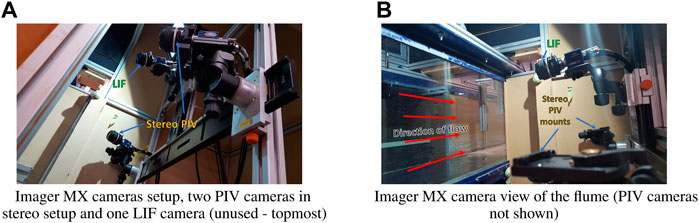
FIGURE 1. PIV camera setup for experimental flow validation. (A) Imager MX cameras setup, two PIV cameras in stereo setup and one LIF camera (unused - topmost) (B) Imager MX camera view of the flume (PIV cameras not shown).

Acoustic Doppler Velocimetry (ADV) sensing was used at 7, 8 and 9 m from the upstream inlet to ensure the flow was fully developed prior to the PIV measurement section. At each streamwise position, the ADV probe was placed at 4 mm vertical intervals inside the flow and measured the velocity at 100 Hz. Once the ADV was used to check the flow was fully developed, the probe was removed to avoid disturbance of the flow entering the PIV measurement section. ADV data collected from the 9 m location was used to compare against the PIV results.

Figure 2 shows the sensors used in the experimental tests.

FIGURE 2

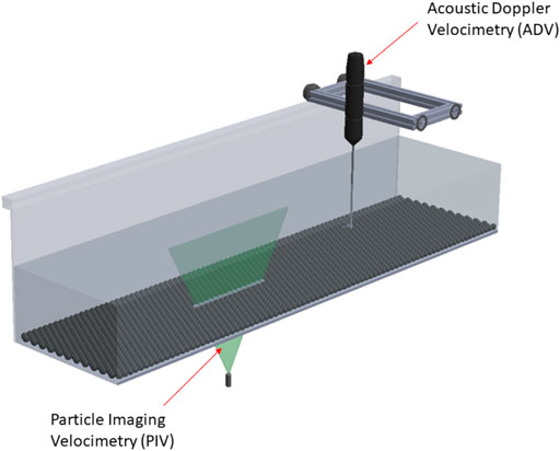
FIGURE 2. Experimental setup. The Particle Imaging Velocimetry (PIV) and Acoustic Doppler Velocimetry (ADV) were used to measure flow properties. Properties.

2.2 CFD setup

2.2.1 Bed geometry and mesh creation

A bed of physical roughness elements was created using hexagonal packed spheres with a radius, r of 12 mm.

Since the majority of the turbulence generation occurs from the upper half of the spheres, in the CFD simulation only the upper parts are used. As shown in Figure 3A, the spheres touch at a tangential point which causes issues with the mesh. To allow a small distance between each sphere (d₂ = 0.5 mm), the spheres are further sunken into the bed. This assists in creating a good mesh without requiring infinitesimally small elements. By using Pythagoras’ theorem, Eq. 2 was used to calculate the distance, t which the hemi-spheres need to be sunk into the bed.

$d_1=r-\frac{d_2}{2}(1)$

$t=\sqrt{r^2-{\left(d_1\right)}^2}=4.8734\mathrm{m}\mathrm{m}(2)$

FIGURE 3

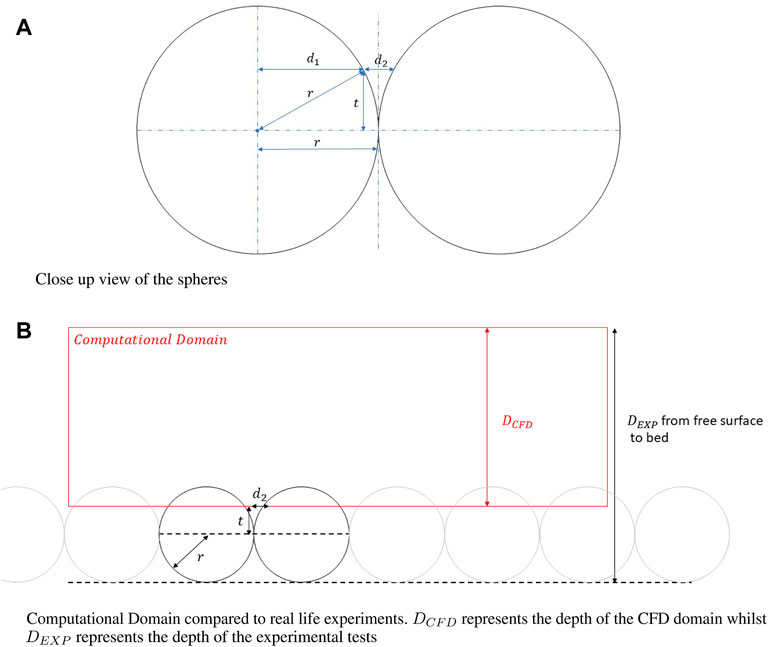
FIGURE 3. Diagram showing the submergence of the virtual bed below the bed of spherical roughness elements. r is the radius of the spherical roughness element, d₂ is the distance between the spherical roughness elements at a given distance t above the centerline of the spheres and d₂ is the adjacent length of the right angle triangle formed by the sides makred r and t. Eq. 2 states geometric relations between these variables to enable calculation of t. (A) Close up view of the spheres (B) Computational Domain compared to real life experiments. D_CFD represents the depth of the CFD domain whilst D_EXP represents the depth of the experimental tests.

Figure 3B provides a visual comparison of the flow depth between the CFD domain (D_CFD) and the laboratory flume experiments (D_EXP). To move between the computational domain and the experimental domain, Eq. 3 can be used.

$D_{\mathit{CFD}}=D_{\mathit{EXP}}-\left(r+t\right)(3)$

For stage 1, the computational domain was 312 mm in the streamwise direction (13 sphere diameters), 166.24 mm in the transverse direction (8 sphere diameters in hexagonal close packed configuration) and a flow depth of 33 mm (Figure 4). For stage 2, the computational domain was shrunk to 96 mm in the streamwise direction (4 sphere diameters in hexagonal close packed configuration) and 82 mm in the transverse direction (4 spheres). This can be seen in Figure 6. The depth of flow was not changed.

FIGURE 4

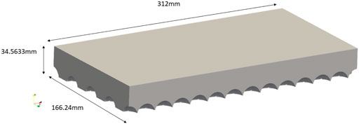
FIGURE 4. Computational domain for stage 1 of the simulation (only 4 spherical cap roughness elements are shown).

To create the mesh, several steps are taken. Firstly, the general computational domain without the rough bed is created using blockMesh.

Secondly, the rough bed is saved as an STL file and imported into OpenFOAM. This is used by the SnappyHexMesh utility to generate a mesh of the rough bed. The edges of the hemi-spheres are extracted and used to refine the mesh around the physical roughness elements. Mesh points which are located inside the physical roughness elements are removed, elements are moved to conform to the bed geometry and additional layers are added around the hemi-spheres to improve near bed performance. The minimum mesh size was originally determined by the desired y + to capture near wall effects. However, it was later discovered that the mesh needed to be much finer than this minimum requirement due to the complex bed geometry. Therefore, the mesh was dictated by the quality of the mesh around these complex bed features. Notably in the second stage of the simulation, the fine mesh is able to fully capture the curvature of the spherical caps even in the small gaps between the spherical cap elements.

Figure 4 and Figure 5 show the computational domain and the mesh created respectively for the stage 1 simulation. Figure 6 shows the refined mesh used for the second stage of the simulation.

FIGURE 5

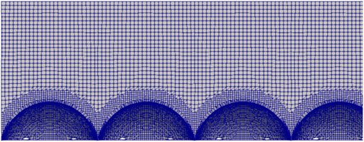
FIGURE 5. Mesh for stage 1 of the simulation, small section of 4 spheres shown.

FIGURE 6

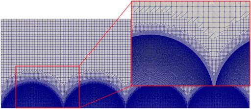
FIGURE 6. Mesh for stage 2 of the simulation (mesh has been refined as shown in the close up view).

2.3 Boundary conditions

The same boundary conditions were applied to both stages of the CFD simulation.

Cyclic (also known as periodic) boundary conditions are applied to the upstream and downstream faces. Any fluid that exits the computational domain immediately re-enters via the upstream face.

As the flow conditions were classified as shallow and the channel’s width is sufficiently larger than the water depth, the sides of the open channel have minimal effect on the center of the flow. Hence, symmetrical conditions were imposed on the side walls of the truncated CFD model. Periodic boundary conditions were considered but not selected to minimise any artificial transverse velocity errors from being propagated and magnified. Based on the conservation of mass, there should be no time averaged net movement of fluid across the open channel in the transverse direction.

A no-slip condition was applied to the bed and the spheres. As discussed above, the free surface was modelled as a rigid lid with symmetry boundary condition applied.

The force applied to the fluid ensures an average velocity of 0.08 m/s (the same as the experimental tests). According to literature, 130 depths are needed for entrance length to develop the flow (Lien et al., 2004). With an effective depth of 25 mm, that would translate to 3.25 m if using the stage 2 smaller computational domain. This would correspond to 3,250 mm/96 mm = 34 FTP. At a bulk flow rate of 0.08 m/s, the time taken is 3.25/0.08 = 40.6 s. However, as the stage 1 RANS simulation is used to initialise the stage 2 LES simulation, the time to reach stabilisation can be reduced slightly.

The first stage RANS simulation was run for 43 s. Monitoring of the local and global residuals was carried out to check for stabilisation and convergence of the simulation whilst comparison to experiments were conducted in the second stage to assess real world compatibility.

The second stage of the simulation using LES was run for a further 50 s before the data was extracted to analyse flow statistics such as velocity, turbulence intensity and Reynolds shear stress.

2.4 Solver

Within OpenFOAM, the pimpleFoam algorithm is used, this combines the PISO (Pressure-Implicit with Splitting of Operators) and SIMPLE (Semi-Implicit Method for Pressure Linked Equations) algorithms. PimpleFoam solves the general momentum equations and is intended for incompressible, single-phase, transient flows (Holzmann, 2019). In this simulation, the momentumPredictor is enabled with nOuterCorrectors = 1 (equivalent to PISO mode), nCorrectors = 2, and nNonOrthogonalCorrectors = 1. A maximum Courant number of 1 was used.

2.5 Computational resources

The simulation was run using OpenMPI at the National Supercomputing Centre in Singapore. ASPIRE-1 (Advanced Supercomputer For Petascale Innovation Research and Enterprise) is a national facility with a 1 PFLOPS System, 1,288 nodes (dual socket, 12 cores/CPU E5-2690v3), 128 GB DDR4 RAM/node and 10 large memory nodes (1x6TB, 4x2TB, 5x1TB). It has a total of 13 PB Storage using GPFS and Lustre File Systems and an I/O bandwidth up to 500 GB/s 6 jobs of 24 h each were submitted using 96 processors across 4 nodes.

Communication within the cluster is achieved with an Infiniband Interconnection EDR (100Gbps) Fat Tree with full bisectional bandwidth.

3 Results and discussion

3.1 Validation

The CFD data was extracted every 0.01 s using the singleGraph function in OpenFOAM. This extracts a line of data within the flow field for further analysis. Figure 7 shows a comparison between the time-averaged streamwise, transverse and vertical velocity profiles from the CFD simulation against PIV and ADV measurements.

FIGURE 7

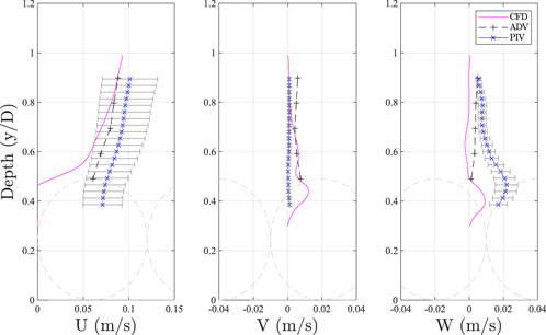
FIGURE 7. Comparison of mean velocity profile. Rough bed has been added in for visual effect only. U is the velocity in the streamwise direction, V is the velocity in the vertical direction and W is velocity in the transverse or spanwise direction.

The PIV data shown in Figure 7 was extracted in a single vertical line and not spatially averaged. The ADV measurements used for validation in this section were taken at 9 m downstream from the inlet. ADV and PIV methods have different types of errors. For example, the PIV method is affected by the image quality which influences the accuracy of the vector field calculation. Error bars have been added to the PIV to demonstrate the expected uncertainty of the velocity. It can be seen that in the streamwise direction, the CFD and the ADV data is within the PIV measurement margin of error.

Figure 8 shows a similar comparison for turbulence intensity, TI. This was calculated using Eq. 4 where U′ is the instantaneous velocity fluctuation in the streamwise direction and U_shear is the shear velocity.

$TI=\sqrt{\overline{U^{\prime 2}}}/U_{\mathit{shear}}(4)$

FIGURE 8

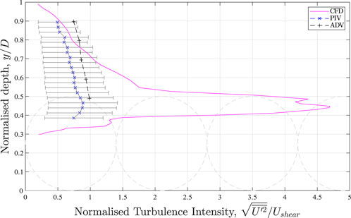
FIGURE 8. Comparison of Turbulence Intensity profile. Rough bed has been added in for visual effect only.

Here, it can be observed that the turbulence is very large between the spherical caps. This cannot be validated using the experimental data because the PIV and ADV are only able to provide reliable data above the spheres. The PIV cameras do not have line of sight to see deep in between the spheres and the ADV probe and its sampling volume is too large to fit in between the spheres. The position of the bed (d2) in the CFD domain is virtual with the actual bed (from the experiments) located at the bottom of the spheres (which is outside the computational domain and not modelled). Therefore, it is possible that the no-slip condition on the virtual bed caused a magnification of the shear gradient which was not present in the same position compared to the experimental tests. Note that the focus here is on the free surface, however future work should use a slip condition to minimise potential effects. Figure 9 shows a comparison with the Reynolds’ shear stress calculated using Eq. 7 where RS_i is the Reynolds’ shear stresses with subscript i being the different cross products. ρ is the density of water, V′ and W′ are the vertical and transverse velocity fluctuations respectively.

FIGURE 9

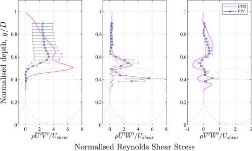
FIGURE 9. Comparison of Reynolds Stress profile. Rough bed has been added in for visual effect only.

The ADV method is affected by vibration of the flume apparatus due to the operation of the water pump. Therefore it was not used for validation of the higher order flow statistics.

$\begin{array}{ll}\hfill R{S}_{uv}& =\rho \overline{U^{\prime }{V}^{\prime }}/U_{\mathit{shear}}\hfill \end{array}(5)$

$\begin{array}{ll}\hfill R{S}_{uw}& =\rho \overline{U^{\prime }{W}^{\prime }}/U_{\mathit{shear}}\hfill \end{array}(6)$

$\begin{array}{ll}\hfill R{S}_{vw}& =\rho \overline{V^{\prime }{W}^{\prime }}/U_{\mathit{shear}}\hfill \end{array}(7)$

Whilst the CFD and the experimental tests follow similar trends, the Reynolds shear stresses near the rigid lid free surface are subdued. The rigid lid imposes zero vertical fluctuation as a boundary, therefore, the vertical velocity fluctuation at the rigid lid will always be zero. Referring back to Figure 7, this can also be observed as the CFD vertical velocity profile (middle pane), ends with zero velocity at the free surface. Since the equation for RS_uv includes the term V′, it is a mathematical inevitability that RS_uv near the free surface is reduced to zero. This effect is evident in Figure 9 from a normalised depth from 1 to 0.7 (Y = 49 mm to Y = 34.3 mm) suggesting that the turbulence data in this region is inaccurate. This would affect any sediment transportation effects and possibly wider turbulent structure interaction. Figure 10 shows the power spectra analysis of the streamwise velocity fluctuation taken at X = 0, Y = 32 mm, Z = 0. The nonparametric, periodogram Welch method by Welch (1967) was used. Kolmogorov’s -5/3 power law is also shown to indicate the turbulent dissipation across the energy spectrum. Data was extracted every 0.01 s (100 Hz). As can be seen from the power spectra, most of the energy is concentrated in the low frequency region of the spectra which suggests that the sampling interval is sufficient. The results show a reasonable capture of the turbulent energy cascade within the CFD simulation. This suggests that the turbulence energies are simulated correctly.

FIGURE 10

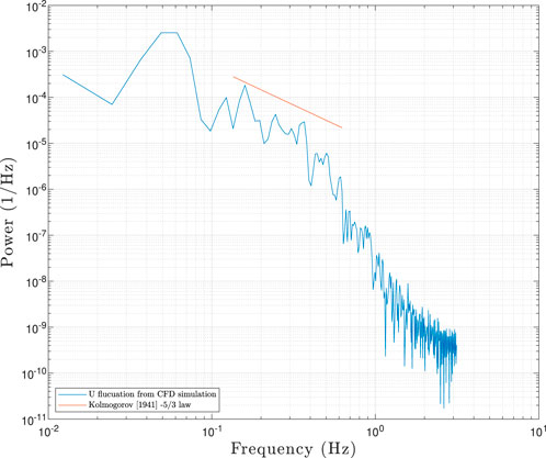
FIGURE 10. Power Spectra Analysis of streamwise velocity fluctuation taken at spanwise centerline, 2.5 mm below the free surface (X = 0, Y = 0.032, Z = 0).

3.2 Vortex analysis

Time series analysis was conducted by visual observation of flow snapshots and identifying the movement of coherent structures.

Figure 11A uses the Q-criterion method with a threshold of 40. Proposed by Hunt et al. (1988), Q-criterion is a variable which describes the main motion pattern of a fluid element. For Q $>$ 0, the rotation motion dominates, whilst for Q $<$ 0, the deformation motion dominates. The vortex flow has the character of Q $>$ 0, but not all regions with Q $>$ 0 are vortex flow regions. Previous studies such as Nagaosa and Handler (2003); Miura and Kida (1997); Jeong and Hussain (1995); Tanaka and Kida (1998) have demonstrated that a manual selection a non-zero threshold can visualise more appropriate structures in flow. The same approach is utilised here with different thresholds tested to assess the number of structures identified. Using a Q-criteron threshold of 40, it can be seen that numerous vortex-like structures are present within the flow. A similar analysis was carried out using the Lambda2 vortex detection method. The same time step is shown in Figure 11B. This method was proposed by Jeong and Hussain (1995) and is essentially a vortex core line detection algorithm which defines a vortex in terms of eigenvalues of the symmetric tensor. It captures the pressure minimum in a plane perpendicular to the vortex axis at high Reynolds numbers. Furthermore, unlike a pressure-minimum criterion, the lambda2 method claims to accurately define vortex cores at low Reynolds numbers. This is important for the current application as the flow is not highly turbulent. Seddighi et al. (2015) was able to use the lambda2 method for identifying vortices in channel flows with regular pyramidal roughness elements.

FIGURE 11

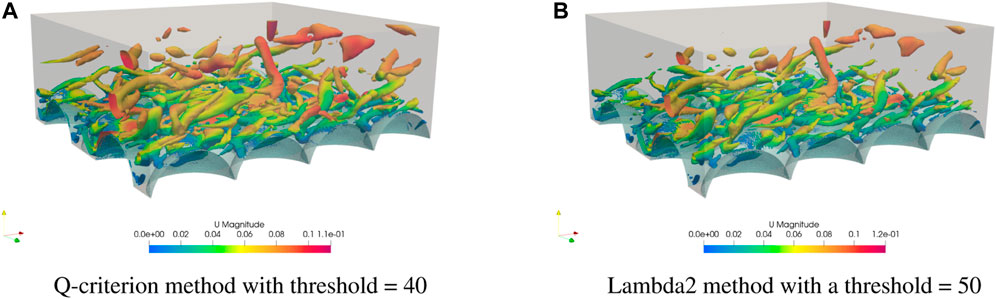
FIGURE 11. Vortex Detection methods at 89.54 s. (A) Q-criterion method with threshold = 40 (B) Lambda2 method with a threshold = 50.

In both figures, it can be observed that the vortices identified are similar in number, scale and shape. For both methods, the threshold value has been selected to identify vortices near the bed. Lowering the Q-criteron threshold enables more of the flow to be identified as a vortex. A frame by frame analysis using a lower Q-criteron is shown in Figure 12. Time steps of 0.1 s are shown from 36.1 s to 36.4. It can be seen that the vortices are clearly rising from the bed whilst being deformed in the streamwise direction by the bulk flow. From 36.1 to 36.3 s, the effect of the turbulent structure hitting the rigid lid water surface can also be observed. These coherent structures clearly hit the underside of the water surface before being propagated in the streamwise direction with the bulk flow.

FIGURE 12

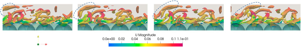
FIGURE 12. Consecutive frames from 36.1 to 36.4 at 0.1 s intervals using Q-criteron with threshold = 20. Only structures in a 0.02 m slice section are shown (taken from −0.01 m to 0.01 m in the spanwise direction).

Assessing this further, Figure 13 shows the simulation domain with a top view using Lambda2 with threshold = 10. A horizontal flat plane is taken 2.5 mm below the free surface with the colours representing the velocity in the vertical direction. It can be observed that the presence of turbulent structures often coincides with the green coloured regions. This suggests that 1) turbulent structures move with a different vertical velocity to the bulk flow and 2) will hit the free surface (given the proximity of the horizontal plane with the free surface).

FIGURE 13

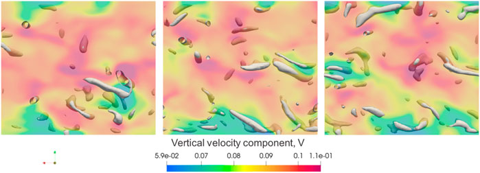
FIGURE 13. Top view using Lambda with threshold = 10. Selected frames at 23.68, 36.0 and 36.9 s from left to right. Coloured by vertical velocity. Horizontal plane taken 2.5 mm below the free surface. Areas of vertical velocity appear to correlate with the presence of local turbulent structures.

By studying the creation and movement of turbulent structures using different Q-criteron thresholds, it is clear that the turbulent structures that are generated at the bed do occasionally grow to enough magnitude to break through the near surface water layer and impinge on the water surface above. Since a rigid lid has very different properties to a flexible lid, it can be said that the rigidity of the lid will lead to an unrealistic response of the turbulent structure as it impacts the free surface. The impingement of the turbulent structures on a free surface would be expected to generate at least some upwards deformation of the free surface shortly followed by a downwards deformation due to the gravitational force and surface tension pulling the flexible lid back downwards. The fluctuation of the free surface would likely transmit some force or pressure onto the coherent structure possibly causing it to re-enter the central part of the flow and possibly triggering new bursts at the bed to restart the cycle again.

Conceptually, if the flow is visualised “upside-down” such that the free surface becomes the “bed”, then should be clear that the underside of the water-air interface is also dynamically “rough”. When the bulk flow attempts to move past this turbulent rough movement, it is inevitable that the bulk flow is affected by the underside of the free surface. In wave propagation theory, a wave is referred to as “smooth” if its wavelength is considered “long” with respect to the turbulence length scales. However, if the length scale of wave is similar to eddy length scales, from the perspective of the flow, the surface appears very rough. In the framework proposed by Brocchini and Peregrine (2001), they suggest that these specific shallow flow conditions create small surface fluctuations. Based on the Reynolds’ number, empirical turbulent sub-layer studies and analysis conducted in the present study, it is clear that the dominant turbulent scales are also relatively small and of similar scale to the free surface fluctuation. Therefore, the use of a rigid lid will certainly have a noticeable effect on the re-distribution of turbulent energies from coherent structures as they impinge on the free surface.

Unlike experiments, CFD time steps can be saved and restarted to obtain the same results. These time step files can also be used in a different simulation with little loss in accuracy. Therefore a logical future step could be to take a timestep containing large vortex before it impacts the free surface (e.g. 36 s into the simulation). A new simulation with a flexible free surface could be started using this time step to compare the response of the structure with and without a rigid lid. Results from a free surface simulation can further investigate the hypothesis that roughness on the free surface is generated and determine if rigid lids could still be used in future simulations.

4 Conclusion

CFD simulations have been developed to study the effect of rigid lids on turbulent structures in open channel flows with a rough bed. A two stage approach was used whereby a coarse mesh was created for an initial RANS simulation to develop flow statistics before a second stage used a fine mesh with LES to develop transient turbulent structures. Both the time averaged velocity profiles and the turbulent intensities simulated correlate well with experimental results. However, Reynolds’ shear stresses associated with the vertical velocity fluctuation are artificially reduced to zero near the rigid lid. This is due to the boundary condition forcing zero vertical velocity at the rigid lid leading to no vertical fluctuations. This was shown to affect the flow from a normalised depth of 1 (at the free surface) to 0.7 (30% below the free surface).

Finally, it was visually shown that turbulent structures that are generated at the bed can impinge on the rigid lid. Once this occurs, the structure is then pinned at the lid and dragged along by the bulk flow until the structure dissipates. Were the lid to be flexible and representative of a real free surface, the response of the turbulent structures are expected to be different. It is believed that the findings are applicable to a range of similar flows (shallow). More work is necessary to repeat the simulation with different depths and flow rates to confirm this. Future steps should take a time step with a large turbulent structure rising towards the free surface and run a flexible free surface simulation to directly compare the differences in the response of the coherent structure after contact with the rigid/flexible free surface.

Data availability statement

The original contributions presented in the study are publicly available. This data can be found and generated using code here: https://github.com/Yun-HangCho/-Computational-Fluid-Dynamics-Simulation-of-Rough-Bed-Open-Channels-Using-OpenFOAM.

Author contributions

Y-HC developed the CFD model and wrote the paper. MD and AN supervised and edited the paper.

Funding

The computational work for this article was (fully/partially) performed on resources of the National Supercomputing Centre, Singapore (https://www.nscc.sg) (Accessed via the Institute of High Performance Computing at the Agency for Science, Technology and Research (ASTAR).

Acknowledgments

Many thanks to the ASTAR Graduate Academy and the University of Sheffield for their funding of this research. Sincere appreciation to Arthur Hajaali at UCL for the technical support and advice.

Conflict of interest

The authors declare that the research was conducted in the absence of any commercial or financial relationships that could be construed as a potential conflict of interest.

Publisher’s note

All claims expressed in this article are solely those of the authors and do not necessarily represent those of their affiliated organizations, or those of the publisher, the editors and the reviewers. Any product that may be evaluated in this article, or claim that may be made by its manufacturer, is not guaranteed or endorsed by the publisher.

References

Adrian, R., Meinhart, C., and Tomkins, C. (2000). Vortex organization in the outer region of the turbulent boundary layer. J. Fluid Mech. 422, 1–54. doi:10.1017/S0022112000001580

CrossRef Full Text | Google Scholar

Alfonsi, G., Ferraro, D., Lauria, A., and Gaudio, R. (2019). Large-eddy simulation of turbulent natural-bed flow. Phys. Fluids 31, 085105. doi:10.1063/1.5116522

CrossRef Full Text | Google Scholar

Bomminayuni, S., and Stoesser, T. (2011). Turbulence statistics in an open-channel flow over a rough bed. J. Hydraul. Eng. 137, 1347–1358. doi:10.1061/(ASCE)HY.1943-7900.0000454

CrossRef Full Text | Google Scholar

Borue, V., Orszag, S. A., and Staroselsky, I. (1995). Interaction of surface waves with turbulence: Direct numerical simulations of turbulent open-channel flow. J. Fluid Mech. 286, 1–23. doi:10.1017/S0022112095000620

CrossRef Full Text | Google Scholar

Brocchini, M., and Peregrine, D. H. (2001). The dynamics of strong turbulence at free surfaces. Part 1. Description. J. Fluid Mech. 449, 225–254. doi:10.1017/S0022112001006012

CrossRef Full Text | Google Scholar

Burg, D., and Ausubel, J. H. (2021). Moore’s law revisited through intel chip density. PLOS ONE 16, 02562455–e256318. doi:10.1371/journal.pone.0256245

CrossRef Full Text | Google Scholar

Dao, M. H., Chew, L. W., and Zhang, Y. (2018). Modelling physical wave tank with flap paddle and porous beach in openfoam. Ocean. Eng. 154, 204–215. doi:10.1016/j.oceaneng.2018.02.024

CrossRef Full Text | Google Scholar

Grass, A. J. (1971). Structural features of turbulent flow over smooth and rough boundaries. J. Fluid Mech. 50, 233–255. doi:10.1017/S0022112071002556

CrossRef Full Text | Google Scholar

Holzmann, T. (2019). Mathematics, numerics, derivations and OpenFOAM® (holzmann CFD).

Google Scholar

Horoshenkov, K. V., Nichols, A., Tait, S. J., and Maximov, G. A. (2013). The pattern of surface waves in a shallow free-surface flow. J. Geophys. Res. Earth Surf. 118, 1864–1876. doi:10.1002/jgrf.20117

CrossRef Full Text | Google Scholar

Horoshenkov, K. V., Van Renterghem, T., Nichols, A., and Krynkin, A. (2016). Finite difference time domain modelling of sound scattering by the dynamically rough surface of a turbulent open channel flow. Appl. Acoust. 110, 13–22. doi:10.1016/j.apacoust.2016.03.009

CrossRef Full Text | Google Scholar

Hunt, J., Wray, A., and Moin, P. (1988). “Eddies stream, and convergence zones in turbulent flows,” in Proceedings of the 1988 summer program.

Google Scholar

Jeong, J., and Hussain, F. (1995). On the identification of a vortex. J. Fluid Mech. 285, 69–94. doi:10.1017/S0022112095000462

CrossRef Full Text | Google Scholar

Jimenez, J. (2004). Turbulent flows over rough walls. Annu. Rev. Fluid Mech. 36, 173–196. doi:10.1146/annurev.fluid.36.050802.122103

CrossRef Full Text | Google Scholar

Kazemi, E., Koll, K., Tait, S., and Shao, S. (2020). Sph modelling of turbulent open channel flow over and within natural gravel beds with rough interfacial boundaries. Adv. Water Resour. 140, 103557. doi:10.1016/j.advwatres.2020.103557

CrossRef Full Text | Google Scholar

Kline, S., Reynolds, W., Schraub, F., and Runstadler, P. (1967). The structure of turbulent boundary layers. J. Fluid Mech. 30, 741–773. doi:10.1017/s0022112067001740

CrossRef Full Text | Google Scholar

Komori, S., Murakami, Y., and Ueda, H. (1989). The relationship between surface-renewal and bursting motions in an open-channel flow. J. Fluid Mech. 203, 103–123. doi:10.1017/S0022112089001394

CrossRef Full Text | Google Scholar

Lamb, H. (1993). Hydrodynamics. New York: Cambridge University Press.

Google Scholar

Lien, K., Monty, J., Chong, M., and Ooi, A. (2004). “The entrance length for fully developed turbulent channel flow,” in 15th Australasian Fluid Mechanics Conference.

Google Scholar

Miura, H., and Kida, S. (1997). Identification of tubular vortices in turbulence. J. Phys. Soc. Jpn. 66, 1331–1334. doi:10.1143/JPSJ.66.1331

CrossRef Full Text | Google Scholar

Muraro, F., Dolcetti, G., Nichols, A., Tait, S. J., and Horoshenkov, K. V. (2021). Free-surface behaviour of shallow turbulent flows. J. Hydraulic Res. 59, 1–20. doi:10.1080/00221686.2020.1870007

CrossRef Full Text | Google Scholar

Nagaosa, R. (1999). Direct numerical simulation of vortex structures and turbulent scalar transfer across a free surface in a fully developed turbulence. Phys. Fluids 11, 1581–1595. doi:10.1063/1.870020

CrossRef Full Text | Google Scholar

Nagaosa, R., and Handler, R. (2003). Statistical analysis of coherent vortices near a free surface in a fully developed turbulence. Phys. Fluids (1994). 15, 375–394. doi:10.1063/1.1533071

CrossRef Full Text | Google Scholar

Nichols, A., Rubinato, M., Cho, Y., and Wu, J. (2020). Optimal use of titanium dioxide colourant to enable water surfaces to be measured by kinect sensors. Sensors (Basel). 20, 3507–3517. doi:10.3390/s20123507

PubMed Abstract | CrossRef Full Text | Google Scholar

Nichols, A., and Rubinato, M. (2016). Remote sensing of environmental processes via low-cost 3D free-surface mapping. Liege, Belgium: 4th IHAR Europe Congress, 27.

Google Scholar

Nichols, A., Tait, S., Horoshenkov, K., and Shepherd, S. (2013). A non-invasive airborne wave monitor. Flow Meas. Instrum. 34, 118–126. doi:10.1016/j.flowmeasinst.2013.09.006

CrossRef Full Text | Google Scholar

Nicoud, F., and Ducros, F. (1999). Subgrid-scale stress modelling based on the square of the velocity gradient tensor. Flow. Turbul. Combust. 62, 183–200. doi:10.1023/A:1009995426001

CrossRef Full Text | Google Scholar

Roy, A., Buffin-Belanger, T., Lamarre, H., and Kirkbride, A. D. (2004). Size, shape and dynamics of large-scale turbulent flow structures in a gravel-bed river. J. Fluid Mech. 500, 1–27. doi:10.1017/s0022112003006396

CrossRef Full Text | Google Scholar

Satoru, K., Hiromasa, U., Fumimaru, O., and Tokuro, M. (1982). Turbulence structure and transport mechanism at the free surface in an open channel flow. Int. J. Heat Mass Transf. 25, 513–521. doi:10.1016/0017-9310(82)90054-0

CrossRef Full Text | Google Scholar

Savelsberg, R., and van de Water, W. (2008). Turbulence of a free surface. Phys. Rev. Lett. 100, 034501. doi:10.1103/PhysRevLett.100.034501

PubMed Abstract | CrossRef Full Text | Google Scholar

Seddighi, M., He, S., Pokrajac, D., O’Donoghue, T., and Vardy, A. E. (2015). Turbulence in a transient channel flow with a wall of pyramid roughness. J. Fluid Mech. 781, 226–260. doi:10.1017/jfm.2015.488

CrossRef Full Text | Google Scholar

Singh, K. M., Sandham, N. D., and Williams, J. J. R. (2007). Numerical simulation of flow over a rough bed. J. Hydraul. Eng. 133, 3864–4398. doi:10.1061/(asce)0733-9429(2007)133:4(386)

CrossRef Full Text | Google Scholar

Stoesser, T., and Rodi, W. (2007). Large eddy simulation of open-channel flow over spheres. Springer Berlin Heidelberg. doi:10.1007/978-3-540-36183-1_23

CrossRef Full Text | Google Scholar

Tan, S. K., Cheng, N.-S., Xie, Y., and Shao, S. (2015). Incompressible sph simulation of open channel flow over smooth bed. J. Hydro-environment Res. 9, 340–353. doi:10.1016/j.jher.2014.12.006

CrossRef Full Text | Google Scholar

Tanaka, M., and Kida, S. (1998). Characterization of vortex tubes and sheets. Phys. Fluids A Fluid Dyn. 5, 2079–2082. doi:10.1063/1.858546

CrossRef Full Text | Google Scholar

Welch, P. D. (1967). The use of fast Fourier transform for the estimation of power spectra: A method based on time averaging over short, modified periodograms. IEEE Trans. Audio Electroacoust. 15, 70–73. doi:10.1109/TAU.1967.1161901

CrossRef Full Text | Google Scholar

Xie, Z., Lin, B., Falconer, R. A., Nichols, A., Tait, S. J., and Horoshenkov, K. V. (2021). Large-eddy simulation of turbulent free surface flow over a gravel bed. Jornal Hydraulic Reserach 60, 205. doi:10.1080/00221686.2021.1908437

CrossRef Full Text | Google Scholar

Yue, W., Lin, C.-L., and Patel, V. (2003). Numerical investigation of turbulent free surface flows using level set method and large eddy simulation. Hydroscience & Engineering College of Engineering, The University of Iowa. Ph.D. thesis.

Google Scholar