The Plastic Pathfinder: A macroplastic transport and fate model for terrestrial environments

Land-based plastic waste is the major source for freshwater and marine plastic pollution. Yet, the transport pathways over land remain highly uncertain. Here, we introduce a new conceptual model to forecast plastic transport on land: the Plastic Pathfinder; a numerical model that simulates the spatiotemporal distribution of macroplastic (>0.5 cm) at a river basin scale. The plastic transport driving forces are wind and surface runoff, while plastic transport is resisted by terrain surface friction. The terrain surface friction, a function of the slope and land use, is converted into thresholds that define the critical wind and surface runoff conditions required to mobilize and transport macroplastic waste. When the wind and/or surface runoff conditions exceed their respective thresholds, the model simulates the transport and (re)distribution of plastics, resulting in plastic accumulation hotspots maps and high probability transport route maps. The Plastic Pathfinder contributes to a better mechanistic understanding of plastic transport through terrestrial environments, and upon future calibration and validation, can serve as a practical tool to optimize plastic waste prevention, mitigation, and reduction strategies.

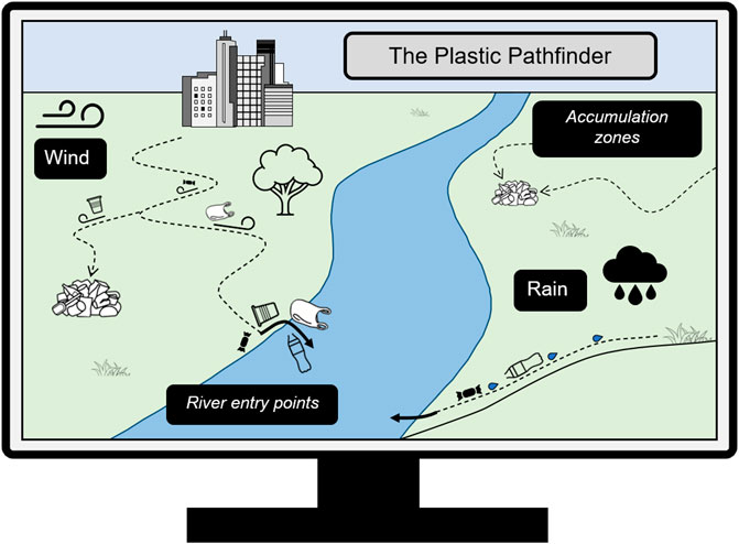
GRAPHICAL ABSTRACT

GRAPHICAL ABSTRACT

1 Introduction

Plastic pollution causes harm to wildlife, through ingestion or entanglement (Sigler, 2014). Human health and livelihood in general is threatened as well, directly through for example the consumption of contaminated seafood (Vethaak and Leslie, 2016; Ribeiro et al., 2020). But also indirectly, for example the increased flood risk in urban areas due to plastic waste clogging the drains (Njeru, 2006; van Emmerik and Schwarz, 2019). Furthermore, economic activities feel negative effects as well, for example when plastic debris damages vessels or when heavily polluted beaches repel tourists. When high production rates and extensive usage of plastics exceed the capacity of the (local) waste management systems, when waste is leaking from dumps or open uncontrolled landfills, or when waste is littered, we refer to it as mismanaged plastic waste (MPW) (Geyer et al., 2017). Each year vast amounts of MPW with a land-based source enter the natural environment, where it is transported across terrestrial systems by aeolian and aquatic processes (Lebreton et al., 2017; Schmidt et al., 2017; Barboza et al., 2019; van Emmerik et al., 2019; Materić et al., 2020). It is assumed that MPW generated on land is the main source of riverine and marine plastic pollution (Biermann et al., 2020; Lau et al., 2020; Wayman and Niemann, 2021). However, several studies suggest that a fraction of the MPW is retained in terrestrial and freshwater systems (Tramoy et al., 2020; van Emmerik et al., 2022). Plastic transport and emission models have been developed over the past years to make an estimate on the amount of MPW that is emitted to the oceans via river emissions (Lebreton et al., 2017; Schmidt et al., 2017). These models use estimates of the MPW generation within a river basin and, combined with waste management, population and hydrological related variables, predict the fraction of MPW that is emitted to the ocean at the river mouth. In other words, they look at what comes in and predict what comes out, but do not take any overland transport and accumulation processes into account. Meijer et al. (2021) was the first to examine in more detail what happens in between the MPW production on land and the emission to the ocean. Their modelling study produces transport probability maps, which indicate for each location in the river basin the probability that MPW produced at that location would be emitted into the oceans within 1 year. By applying their model to hundreds of rivers globally, Meijer et al. (2021) estimate that less than 2% of the land-based MPW annually produced within river basins is emitted to the oceans. While their study offers valuable insights into the probability of plastic transport through river basins, the exact transport routes and accumulation hotspots of the remaining 98% remain unknown.

As of today, there are no plastic transport models that simulate the trajectories of MPW between these terrestrial compartments (Wayman and Niemann, 2021), whereas such models have already been successfully developed for the marine environment (Lebreton et al., 2012; Maximenko et al., 2012; van Sebille et al., 2012; Hardesty et al., 2017; Delandmeter and van Sebille, 2019; Onink et al., 2021). Therefore, we developed the Plastic Pathfinder, a macroplastic transport and fate model that simulates the pathways and spatiotemporal distribution of MPW within the terrestrial parts of river basins. The model concept is based on the assumption that macroplastic waste is mobilized and transported when the driving forces, in this case wind and surface runoff, overcome the terrain friction caused by the (combination of the) terrain slope and type of land use. Our model additionally identifies where terrestrial pollution enters freshwater systems, which makes it valuable for the coupling with existing freshwater plastic transport models. In this paper, we introduce the basic concepts of the Plastic Pathfinder and demonstrate its use through application to an idealized case study. Besides the significant contribution to a better fundamental understanding of plastic transport and accumulation in terrestrial systems, the Plastic Pathfinder is a useful tool for developing and improving (inter)national plastic monitoring, collection and mitigation strategies.

2 Materials and methods

The model is written in Python 3.8.3 in the Jupyter Notebook (Version 6.0.3) environment, a package from Anaconda Navigator (Anaconda Software Distribution, 2016). The code of the Plastic Pathfinder and the user’s manual are available at https://doi.org/10.5281/zenodo.6470410. Below, we introduce the model concept, framework, input, and output. In addition, we present an idealized case study for which we used real-world forcing input data. This model application is meant to illustrate the performances of the Plastic Pathfinder for a simple hypothetical river basin (‘a proof of principle’).

2.1 Model concept

The model concept is based on a principal criterion in the field of sedimentology, which states that sediment motion is initiated when driving forces overcome resistive forces (Shields, 1936). We assume that the motion of macroplastics over land is a function of driving and resistive forces as well and that thresholds mark the conditions required for incipient motion (Figure 1). The two driving forces in the model are wind ($W$) and surface runoff ($SR$) [the same driving forces were used by Meijer et al. (2021)] and the resisting force, i.e., the terrain friction, is a result of the combination of land use and terrain slope, which is translated to a wind ($W_{thres}$) and a surface runoff threshold ($S{R}_{thres}$). For each geographic location in the river basin, the wind speed ($W$) and surface runoff flux ($SR$) are compared with their respective thresholds. This comparison has four possible outcomes:

$\left\{\begin{array}{cc}W< W_{thres} \wedge SR < S{R}_{thres}\hfill & \hfill \left(1\right)\\ W\ge W_{thres} \wedge SR < S{R}_{thres}& \left(2\right)\\ W< W_{thres} \wedge SR \ge S{R}_{thres}& \left(3\right)\\ W\ge W_{thres} \wedge SR \ge S{R}_{thres}& \left(4\right)\end{array}\right.$

FIGURE 1

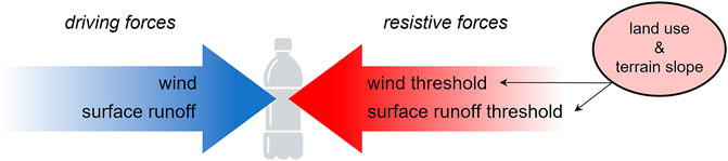
FIGURE 1. Schematic representation of the trade-off between plastic transport driving and resisting forces. The left arrow represents the driving forces, wind and surface runoff, and the right arrow represents the resistive forces, reflected by the wind and surface runoff thresholds. The thresholds are a translation of the resistance induced by the land use and the terrain slope.

In case none of the thresholds are surpassed (Eq. 1), the macroplastics will not be mobilized and no transport occurs. If only the wind threshold is surpassed (Eq. 2), the macroplastics will move in the direction of the wind flow at that geographic location. In case only the surface runoff threshold is surpassed (Eq. 3), the macroplastics will move in the direction of the surface runoff, which is equal to the direction of the steepest downhill terrain slope at that geographic location. Last, if both thresholds are surpassed (Eq. 4), the model randomly picks either the wind or the surface runoff direction as the macroplastic transport direction. The reason for this randomized approach is that no data exists on how to model the relative importance of surface runoff versus wind speed. For example, it is unclear how much surface runoff is required to counteract a certain wind speed. Empirical, future experiments will be necessary to determine the combined effect of wind speed and surface runoff on the net transport (speed and direction) of macroplastics. Consequently, the two plastic transport vectors cannot be combined constructively or destructively as a simple vector product.

2.2 Model framework

The Plastic Pathfinder requires terrain characteristics (including topography and land use), weather conditions (including wind speed/direction and surface runoff), and MPW generation (calculated from population data) (Figure 2). The terrain characteristics in each grid cell of the model domain are translated to a plastic mobilisation and transport threshold (one threshold for wind driven transport and one threshold for surface runoff driven transport). Subsequently, the wind speed and surface runoff thresholds are compared with the wind speed and surface runoff, respectively (i.e., the weather conditions). The outcome of this comparison, presented in a plastic mobilisation map, is combined with the wind and surface runoff directions in order to simulate the transport pathways and accumulation zones of plastic waste.

FIGURE 2

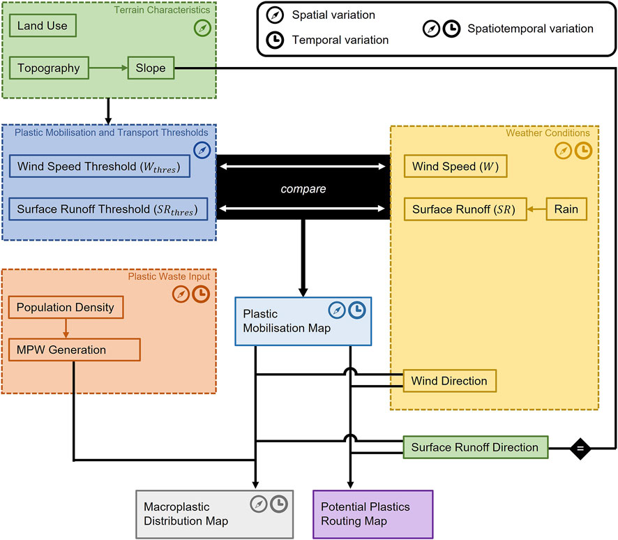
FIGURE 2. Model framework of the Plastic Pathfinder depicting the model in- and outputs.

2.3 Model resolution

The model is built on a rectangular [longitude, latitude] grid, with equally sized grid cells. Input data values, i.e., grid cell properties (e.g., elevation, land use, wind, and rain), are assigned to each grid cell and assumed to be representative for the entire area of land covered by that grid cell. The Plastic Pathfinder can operate on any desired spatial or temporal resolution depending on the required degree of detail and resolution. In our model application, we use a model domain of 30 by 30 arc seconds, a 3 by 3 arc seconds resolution (i.e., 10 by 10 grid cells), a modelled period of 1 year and a temporal resolution of 1 day.

2.4 Modelled directions of motion

All motions modelled by the Plastic Pathfinder occur in the two-dimensional horizontal plane. Analogous to the approach of Jenson and Domingue (Jenson and Domingue, 1988), the modelled components, i.e., air (wind), water (surface runoff) and plastics, can only move from a given grid cell to a neighbouring grid cell. As the model uses a rectangular grid, motion is restricted to eight directions: north, northeast, east, southeast, south, southwest, west and northwest. The fact that the travel distance to diagonal grid cells (i.e., towards the cells in the northeast, southeast, southwest and northwest) is longer than the travel distance to perpendicular grid cells (i.e., towards the cells in the north, east, south and west), is accounted for in the design of the thresholds that control the displacement of plastic waste.

2.5 Model input

2.5.1 Topography

The topography input defines for each grid cell the elevation above sea level in meters. For each grid cell the distance weight drop towards each of its neighbouring grid cells is calculated (topography data can be extracted from a database such as HydroSHEDS (Lehner et al., 2008). The model calculates the distance weighted drop in all eight directions and marks the smallest as the direction of the steepest downhill terrain slope. In case a grid cell is surrounded by grid cells with a higher topography, the smallest distance weighted drop marks the direction of the gentlest uphill slope. The fictional topography map created for the model application and the corresponding steepest downhill slope values (in meter/meter) and directions are shown in Figure 3 a and b, respectively.

FIGURE 3

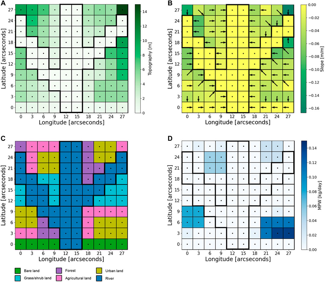
FIGURE 3. (A) Topography input map used in the model application. The map shows for each grid cell the average height above sea level (m). (B) Steepest terrain slope map (calculated from the topography values). The map shows the values of the steepest slope (m/m) and the arrows indicate towards which adjacent grid cell this slope is directed. (C) Land use input map used in the model application. The map shows for each grid cell the type of land use. (D) Mismanaged plastic waste generation input map used in the model application. The map shows for each grid cell the amount of mismanaged plastic waste that is generated during each time step (kg/day). The thick black contours in all four maps indicate the boundaries of the river channel.

2.5.2 Land use

The land use input defines for each grid cell the type of land use. Land use data can be extracted from a database such as the ESA CCI Land Cover time-series (Land Cover CCI Product User Guide Version 2.0, 2017). The Plastic Pathfinder distinguishes between water and five types of land use:

• urban land (artificial surfaces, e.g., cities)

• bare land (little or no vegetation)

• grass/shrub land (grass and/or shrub cover, e.g., pastures)

• agricultural land (edible plants vegetation, e.g., croplands)

• forest (dense vegetation with trees, ranging from tropical rainforests to boreal forests)

These land use categories were selected on the basis of the global Land Cover Themes from the GLC2000 data set (Bartholomé and Belward, 2005). The fictional land use map created for the model application is shown in Figure 3C. The fictional river drains towards a fictional sea in the south and the bare land grid cells (latitude 0) represents a coastline.

2.5.3 Wind

The wind input provides for each time step for a given grid cell the daily averaged wind speed in meters per second and the average wind direction (N, NE, E, SE, S, SW, W or NW). The wind data can be extracted from a database such as the Global Wind Atlas (Global Wind Atlas, 2019) or a local meteorological weather station. Supplementary Table S1 was used to convert the continuous range of wind directions in degrees (0°–360°) to the eight directions of motion used in our model (see section 2.4). The wind speeds (Supplementary Figure S1) and directions (Supplementary Table S2) used for our model application, are based on the frequency of actual wind speeds and directions measured (in the period 1981–2000) at the De Bilt weather station, the Netherlands (frequency tables are available at the KNMI Data Platform (dataplatform.knmi.nl, 2000), the frequency tables used for the wind speeds and wind directions are provided in Supplementary Table S3 and Supplementary Table S4, respectively).

2.5.4 Surface runoff

The surface runoff input provides for each time step for a given grid cell the flux of surface runoff in millimetres per day. Surface runoff data can directly be extracted from a database such as GRUN (Ghiggi et al., 2019) or computed from rainfall data using a surface runoff coefficient. The runoff coefficient (the ratio between runoff and rainfall) is the fraction of the rainwater that does not infiltrate in the soil and can transport plastics along the surface. The type of land cover (i.e., vegetation) plays a major role in this process. The surface runoff direction in each grid cell is equal to the direction of the steepest terrain slope of that grid cell (Figure 3B). The rainfall data used for our model application (Supplementary Figure S2), are based on the frequency of actual amounts of rainfall measured between 1981 and 2000 at the De Bilt weather station, the Netherlands (frequency tables are available at the KNMI Data Platform (dataplatform.knmi.nl, 2000), the frequency table used for the rainfall is provided in Supplementary Table S5). We used typical runoff coefficients to convert the rainfall values into surface runoff values (Goel, 2011; Karamage et al., 2017) (Supplementary Table S6). For our model application we assumed no time lag between a rainfall event and the generation of surface runoff. In some environments, for example in mountainous areas, a time lag between precipitation (e.g. snow) and subsequent generation of surface runoff (e.g. snow melt) is expected. In that case we recommend coupling the Plastic Pathfinder to a hydrodynamic model that takes such time lags between rainfall and the generation of surface runoff into account.

2.5.5 Mismanaged plastic waste generation

The mismanaged plastic waste (MPW) input provides for each time step, for each grid cell, the mass of MPW generated in kilograms. If no MPW generation input data is available, it can be computed from the population density in combination with estimates on the (yearly) generation of solid municipal waste per capita, the fraction of waste that is mismanaged, and the proportion of plastics in solid waste (Lebreton and Andrady, 2019). The fictional population density map used for the model application indicates for each grid cell the number of inhabitants and can be found in Supplementary Figure S3. Forests were assigned an artificial population density of 0.1 people/grid cell (∼12.3 people/km2) in order to account for (occasional) littering associated to recreational activities. The yearly MPW generated in each grid cell was calculated using waste values reported for the Netherlands for the year 2015: 526 kg per capita solid waste production, of which 1% was mismanaged and 19% consisted of plastics (Lebreton and Andrady, 2019). We assumed a constant daily MPW generation and divided the yearly MPW production by 365 in order to obtain the daily MPW generation (Figure 3D).

2.6 Plastic mobilisation and transport thresholds

The Plastic Pathfinder models the mobilisation and transport of plastic waste overland on the basis of thresholds. These plastic mobilisation and transport thresholds mark the point where the driving forces overcome the resistive forces. For both transport agents, i.e., wind speed and surface runoff, we established such thresholds for the mobilisation and transport of plastics on the basis of the combination of topography and land use (Table 1). In general, we assumed that the plastic mobilisation and transport threshold increases with increasing terrain resistance. Below, we describe in more detail how the wind speed and surface runoff thresholds were established.

TABLE 1

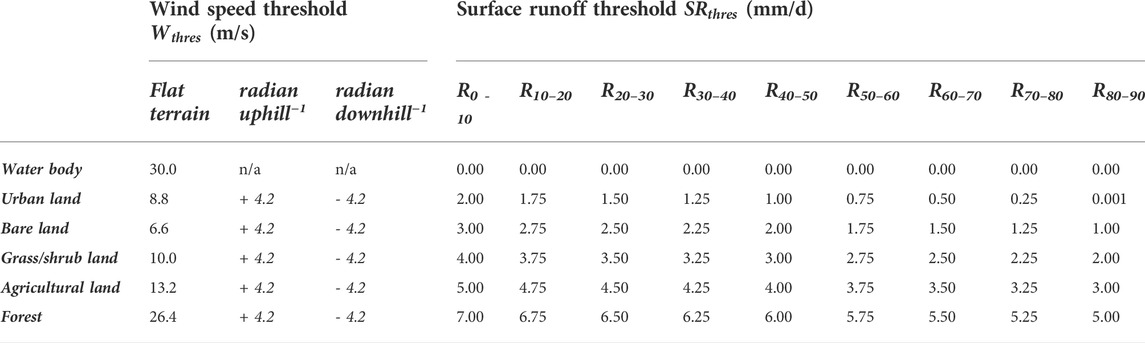
TABLE 1. Wind speed (${\mathit{W}}_{\mathit{thres}}$) and surface runoff threshold ($\mathit{S}{\mathit{R}}_{\mathit{thres}}$) values used by the Plastic Pathfinder. These values indicate for each combination of land use and terrain slope, the critical wind speed (m/s) and surface runoff (mm/d) presumed to mobilise and transport macroplastics. R_x–y refers to the surface runoff threshold for downhill slopes with a slope angle between x and y degrees.

2.6.1 Wind speed thresholds

The wind speed thresholds define the critical wind speed that is presumed to be sufficient to mobilise and transport macroplastics. The wind speed thresholds can be calculated as a function of only the type of land use (option 1) or as a function of the type of land use and the combination of terrain slope and wind direction (option 2). Below we describe both options.

Option 1: Starting point in defining the wind speed thresholds was the Beaufort wind scale, according to which a wind speed around 6.6 m/s (BF4) “raises dust and loose paper” (Met Office, 2010). The density of paper, 1.2 g/cm3, is similar to the density of plastic waste. For example, plastic bottles are made from polyethylene terephthalate, which has a density of 1.37 g/cm3 (Yeo and Hsuan, 2010), and plastic bags are made from low density polyethylene, which has a density between 0.910 and 0.925 g/cm³. Therefore, we established a wind speed threshold of 6.6 m/s for flat bare lands (Table 1). Subsequently, the value of 6.6 m/s was extrapolated in order to obtain the thresholds for the other four land use types. The extrapolation factors were derived from the overland plastic transport probabilities estimated by a panel of 24 experts in a survey conducted by Meijer et al. (2021). The averages of their estimates on the overland transport probability for ‘bare land’, ‘urban’, ‘agricultural land’ and ‘forests’, were 0.96, 0.75, 0.44, and 0.17, respectively. We roughly interpreted these averages as 1.00, 0.75, 0.50 and 0.25 (bare land, urban, agricultural land, and forests). The 6.6 m/s threshold for bare lands corresponds to the probability of 1.00. Subsequently, we established the wind speed thresholds for urban, agricultural land and forests, by multiplying 6.6 m/s with the reciprocals of 0.75, 0.50, and 0.25, respectively (Figure 4). Since the panel of experts was not asked for the overland transport probabilities of plastics across grass/shrub lands, we assumed grass/shrub lands to have a degree of resistance in between urban and agricultural land and established a value between 8.8 m/s and 13.2 m/s: 10.0 m/s. Once plastic waste has entered a water body, e.g., a lake or a river, we assumed that only violent storms and hurricanes can lift and remove plastic waste from the water body. Therefore, a value of 30 m/s was established as wind threshold for water bodies.

FIGURE 4

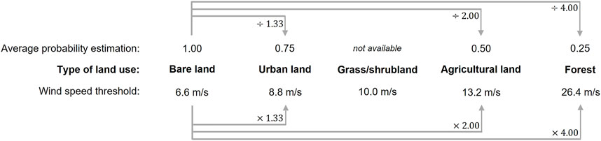
FIGURE 4. Schematic representation of the extrapolation calculation that was performed to obtain the wind speed thresholds for the different land uses. The average probability estimates are derived from a survey conducted by Meijer et al. (2021) in which a panel of experts was asked to estimate the probability of a macroplastic item to be transported across bare, urban, agricultural and forest lands (grass/shrub land was not included).

Option 2: For this calculation of the wind speed threshold it was assumed that the ability of the wind force to mobilise and transport macroplastics (in the direction of the wind) decreases for uphill winds and increases for downhill winds. The reasoning behind this is that in the case of uphill winds, the wind force is counteracted, while for downhill winds it is assisted, by the force of gravity. Therefore, apart from the land use, the topography is taken into account as well. For each radian of terrain slope angle, 4.2 m/s is added (for uphill winds) or subtracted (for downhill winds) from the wind speed thresholds that hold for flat terrains (second column in Table 1). The value of 4.2 m/s was determined by assuming that the wind speed threshold for (hypothetically) vertical bare lands equals 0.0 m/s (free fall). This would imply that a decrease of 6.6 m/s of the wind speed threshold, corresponds to a terrain slope increase of 90° (½π radians). For simplification, we assumed a linear relation, which translates to a decrease of 4.2 m/s for each radian of terrain slope increase. An important implication of this approach is that the wind speed thresholds do not only vary in space, but in time as well, since the wind directions can vary with time. For example, at time t, a certain wind speed at a specific location appears to be insufficient to mobilise and transport macroplastics, while at t+1, the same wind speed but in a different direction appears to be sufficient to surpass the wind speed threshold and consequently displaces the macroplastics.

In our model application we used option 1, i.e., the wind speed thresholds are a function of only the type of land use.

2.6.2 Surface runoff thresholds

The surface runoff thresholds define the critical flux of surface runoff that is presumed to be sufficient to mobilise and transport macroplastics. However, as far as we know, no study to date has examined the mobilisation and transport capacity of surface runoff. We made a first attempt and established the orders of magnitude for the surface runoff thresholds based on the distribution of data on global absolute runoff trends from the Global Runoff Reconstruction (GRUN) model, an observational-based global reconstruction of (monthly) runoff developed by Ghiggi et al. (2019). In urban areas, the smooth surface of asphalt roads and pavements are assumed to exert a low resistance force to the mobilisation and transport of plastics by surface runoff. Therefore, urban areas were assigned with the low surface runoff thresholds ranging from 0.001 mm/day for nearly vertical areas, to 2.00 mm/day for flatter areas (up to 10°) (Table 1). The highest resistance to plastic transport by surface runoff is thought to occur in forests, due to the vegetation that both reduces the surface runoff flow and entraps plastic waste. Therefore, forests were assigned with the highest thresholds ranging from 5 mm/day for steep areas, to 7 mm/day flatter areas (Table 1). We assumed that the steeper the terrain slope, the higher the surface runoff flow velocity and the higher the capability of the surface runoff to mobilise and carry macroplastics. The terrain topography and land use are both constant through time, therefore, the surface runoff thresholds only have a spatial, and not a temporal, variability. Surface runoff driven plastic transport from grid cells that are only surrounded by higher topographies (depressions in the landscape) is assumed impossible. Consequently, plastic waste in those grid cells can only be transported away by the wind.

2.7 Macroplastic transport

The Plastic Pathfinder works with so called MPW clusters, whereby a single MPW cluster consists of all the MPW that was generated in a single grid cell during a single time step. Once MPW is released from its land-based source, it is available for transport. MPW generally consist of different types of plastic waste (e.g., plastic bottles, bags, food wrappers), which are likely to have different mobilisation and transport thresholds. However, the mobilisation and transport thresholds of different types of plastics over land has not been studied up to date. Due to this knowledge gap we were forced to assume uniform mobilisation and transport thresholds that hold for all types of macroplastic waste. This means that the current version of the Plastic Pathfinder simulates the transport and accumulation of a representative subset of macroplastic waste, which is expected not to reflect the transport behaviour of all types of macroplastic waste. As soon as plastic type specific mobilisation and transport thresholds become available, they can replace the uniform thresholds. For each modelled time step during which the wind or surface runoff exceeds their respective threshold, transport is simulated and the entire MPW cluster is displaced from its current grid cell to an adjacent one. When different MPW clusters are transported towards the same grid cell, or when a new MPW cluster is generated in a (land) grid cell in which another MPW cluster was already present, the mass of all those MPW clusters are added. In this way MPW clusters can ‘expand’.

The Plastic Pathfinder only models the transport and accumulation of plastics in terrestrial environments. When the wind or surface runoff forces MPW cluster(s) from a land into a river grid cell, the simulation of its transport ends and the plastics will remain (and fictively accumulate) in that river grid cell. The Plastic Pathfinder can be coupled to hydrological models to simulate the transport (and retention) of plastics in freshwater environments as well.

2.8 Model output

There are three main types of output created by the Plastic Pathfinder. First of all, the wind speed and surface runoff threshold maps that show the critical wind speeds and surface runoff fluxes, respectively, which are required to mobilise and transport macroplastic.

Secondly, there are the spatiotemporal MPW distribution output maps that show for each time step the amount of MPW that is present in each part of the river basin. This type of output depends on the MPW generation input data that was given to the model. The simulated (re)distribution of the MPW mass can be studied on the river basin scale or on a smaller scale, e.g. on the level of individual model grid cells. For the latter, we use the following formula to calculate the MPW stock during each time step of the model simulation:

$MPW stock {\left(t\right)}_{\left[lon,lat\right]}= MPW generation {\left(t\right)}_{\left[lon,lat\right]}+ {\displaystyle \sum }_k^{8}MPW received \left(k\right){\left(t\right)}_{\left[lon,lat\right]} -MPW lost {\left(t\right)}_{\left[lon,lat\right]}(5)$

Where $MPW stock {\left(t\right)}_{[lon,lat]}$ is the total amount of MPW (kg) present in the grid cell at latitude $lat$ and longitude $lon$ by the end of time step $t$, $MPW generation {\left(t\right)}_{[lon,lat]}$ is the total amount of MPW (kg) generated (e.g. littering) in the grid cell at latitude $lat$ and longitude $lon$ at (the start of) time step $t$, $MPW received \left(k\right){\left(t\right)}_{[lon,lat]}$ is the amount of MPW (kg) that the grid cell at latitude $lat$ and longitude $lon$ received from a neighbouring grid cell $k$ (maximum number of eight surrounding grid cells) during time step $t$, and $MPW lost {\left(t\right)}_{\left[lon,lat\right]}$ is the total amount of MPW (kg) that is transported out of the grid cell at latitude $lat$ and longitude $lon$ during time step $t$.

The third type of model output is independent of the MPW generation input data and is presented in a ‘potential plastic routing map’. This output focuses on the potential pathways of macroplastic waste through a river basin.

3 Results

Here, we present the spatiotemporal distributions and transport routes of MPW that we found for our model application. The modelled MPW transport and accumulation are controlled by the values chosen for the plastic mobilisation and transport thresholds (Table 1), which resulted in the wind speed and surface runoff threshold maps shown in Supplementary Figure S4A,B, respectively. We are aware of the fact that those threshold values have no empirical basis yet. Here, we merely intend to demonstrate the potential and applicability of the output of the Plastic Pathfinder model and show that this model can serve as an effective tool to examine how weather conditions can be used to predict the accumulation and transport processes of macroplastics on land.

3.1 Spatiotemporal macroplastic distribution

3.1.1 River basin scale

In our model application, we simulated the (re)distribution of a daily MPW input (Figure 3D) for 365 days. For each time step an MPW distribution map is generated, showing the MPW stock (in kg) present in each grid cell by the end of that time step. The arrows in the MPW distribution maps show in which directions MPW was transported during that time step, whereby the thickness of the MPW transport arrow is linearly proportional to the amount (in kg) of displaced MPW. In general, during rainy days the MPW that is present in the river basin is transported in the direction of the steepest downhill slopes and during windy days the MPW get transported along with the wind. Here, we zoom in on three time steps, all of which have a different set of wind and rain conditions: day 291, 344, and 354 (Figure 5A). On day 291—low wind and high rain–the mobilisation map illustrates that in most grid cells the surface runoff threshold is exceeded (Figure 5E). In those grid cells MPW is transported in the direction of the steepest downhill slopes, i.e., the surface runoff directions (Figures 5B,H). On day 344—high wind and high rain–the mobilisation map illustrates that in the grid cells in the south of the domain both thresholds are exceeded (Figure 5F). As a result, the MPW in those grid cells is transported either in the direction of the wind or the surface runoff (Figures 5C,I) (the model randomly picks between the two). On day 354—high wind and no rain–the mobilisation map reveals that in many grid cells the wind threshold is exceeded (Figure 5G). Accordingly, the MPW in those grid cells is transported in the direction of the wind (Figures 5D,J).

FIGURE 5

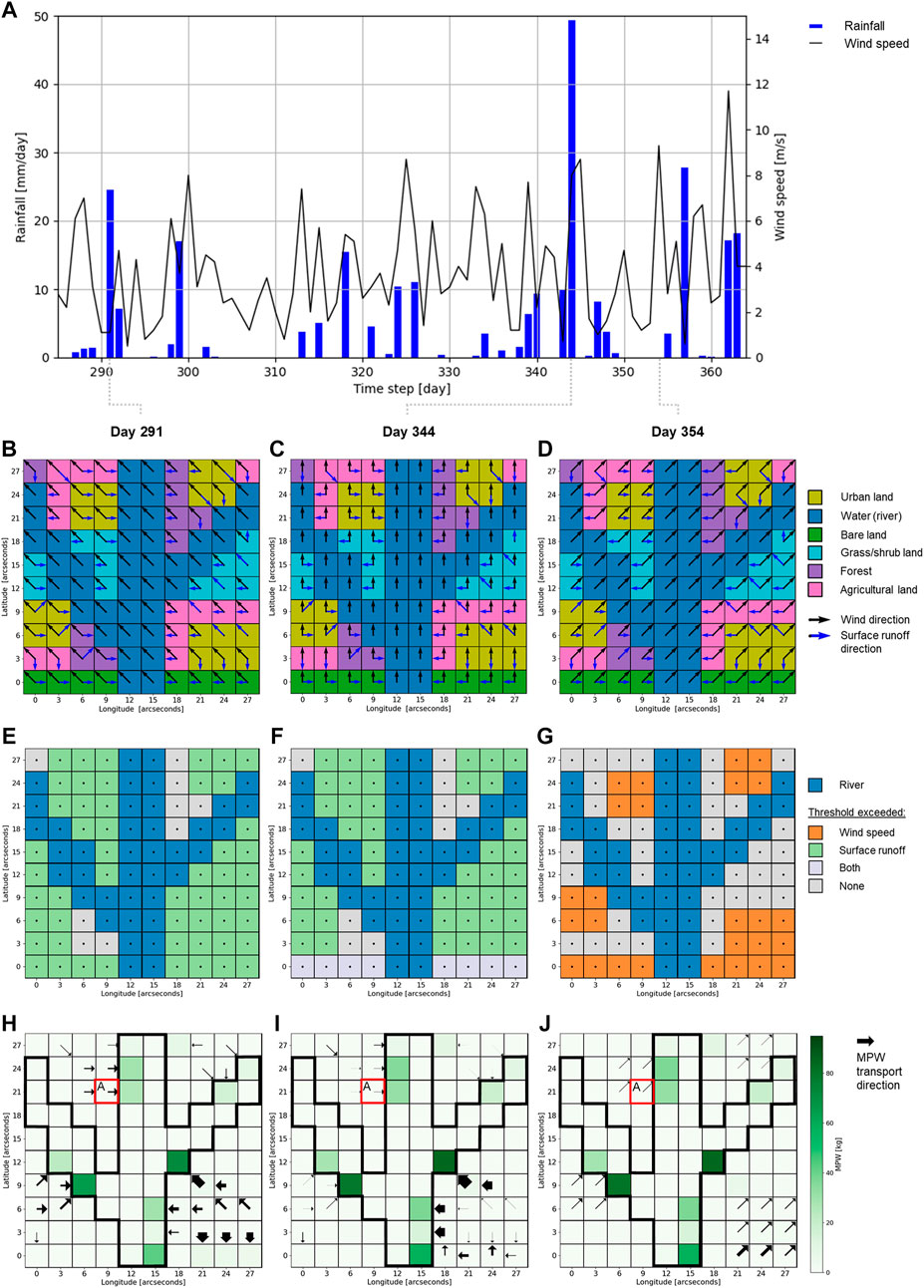
FIGURE 5. (A) Rainfall and wind speeds for the time steps 285 to 364 in the model application. (B), (C), (D) Wind and surface runoff directions for the time steps 291, 344, and 354, respectively. Note how wind direction changes depending on the weather, whereas the surface runoff direction, determined by the topography, remains constant over time. (E), (F), (G) Plastic mobilisation maps for the time steps 291, 344, and 354, respectively. (H), (I), (J) Mismanaged plastic waste (MPW) distribution (kg per grid cell) maps for the time steps 291, 344, and 354, respectively. The arrows show the MPW fluxes (kg/day) that occurred during that time step. The thickness of the arrows is linearly proportional to the magnitude of the MPW flux, i.e., the mass of MPW that was displaced during that day. The red box ‘A’ highlights the grid cell for which an additional local assessment of the MPW evolution has been carried out (see section 3.1.2). The thick black contours in (E) to (J) indicate the boundaries of the river channel.

The spatiotemporal MPW distribution maps provide insights on the MPW transport and when and where MPW accumulates, how long it resides in these terrestrial accumulation zones, and under which (extreme) weather conditions it becomes (re)mobilised/(re)distributed. The Plastic Pathfinder does not simulate the transport of MPW in rivers. The advantage of this is that MPW (fictitiously) accumulates in river grid cells, which subsequently reveals where the main river entry points of MPW are located. For example, in our application the river grid cell at latitude 12 and longitude 18 is a more important entry point of MPW from land to river, than the river grid cell at latitude 21 and longitude 24 (Figures 5H–J).

To understand terrestrial plastic pollution, knowledge on the MPW in- and output fluxes on the catchment scale is necessary. In our model, the input flux consists of the daily MPW input (Figure 3D), and there are three ways for MPW to leave the terrestrial environment: leakage to the river, direct coastal leakage to the ocean, and leakage to adjacent land in the neighbouring watershed. Figure 6A shows these cumulative fluxes through time for our model application, illustrating that the majority of the MPW produced on land reaches the river. This type of output provides valuable insights in the fate of MPW generated on land. Additionally, the distribution of MPW over the terrestrial and freshwater compartments of the river basin can be plotted through time (Figure 6B). This graph shows that after ∼100 days, the MPW stock on land stabilises around a value of 38 kg (STD 16 kg), which implies that the MPW produced on land approximately equals the amount of MPW lost. Please note that no removal processes in the river system were included in the model (e.g., beaching or transport to the ocean).

FIGURE 6

FIGURE 6. (A) Cumulative in- and output fluxes of mismanaged plastic waste (kg) of the terrestrial compartment of the river basin modelled in the model application. The MPW input represents the constant daily on land MPW generation. There are three ways for MPW to leave the terrestrial domain: direct leakage into the river, direct leakage into the ocean, or direct leakage to land from an adjacent river basin (B) The total amount of MPW (kg) present in the entire river basin, i.e., on land and in the river. The green shading represents the amount of MPW (kg) on land and the blue shading corresponds to the amount of MPW (kg) in the river. The black dashed line marks the average amount of MPW (kg) on land during the 365 time steps that were modelled in the model application.

3.1.2 Local scale

Apart from MPW distribution assessments on a river basin scale, the MPW stock of single grid cells can be relevant as well, for example for the design of local measures against terrestrial plastic pollution. Figure 7A shows the MPW in- and output of the urban grid cell located at latitude 21 and longitude 9 (indicated with ‘A’ in Figure 5) for day 200–250. Every day this grid cell receives 0.05 kg of MPW due to in-situ MPW generation (Figure 3D), e.g., littering and inadequate waste collection management. For some days, e.g., 205, 225, and 248, the MPW input exceeds the MPW output (green shading), which means a net accumulation of MPW. While for other days, e.g., 209, 227, and 247, the MPW input is lower than the MPW output (red shading); i.e., a net loss of MPW (Figure 7A). To understand when regions net gain or lose MPW, the weather conditions on these days must be considered. For our model application we found a strong dependency between the amount of rainfall and the net loss of MPW. For example, on day 227 the amount of rainfall is 28.8 mm, and although the cell receives 0.20 kg of MPW from a neighbouring cell, it lost 0.35 kg that day due to surface runoff driven transport. We found that extreme wind speeds, on the other hand, do not necessarily result in a (net) loss of MPW, e.g., day 210 (Figures 7A,B).

FIGURE 7

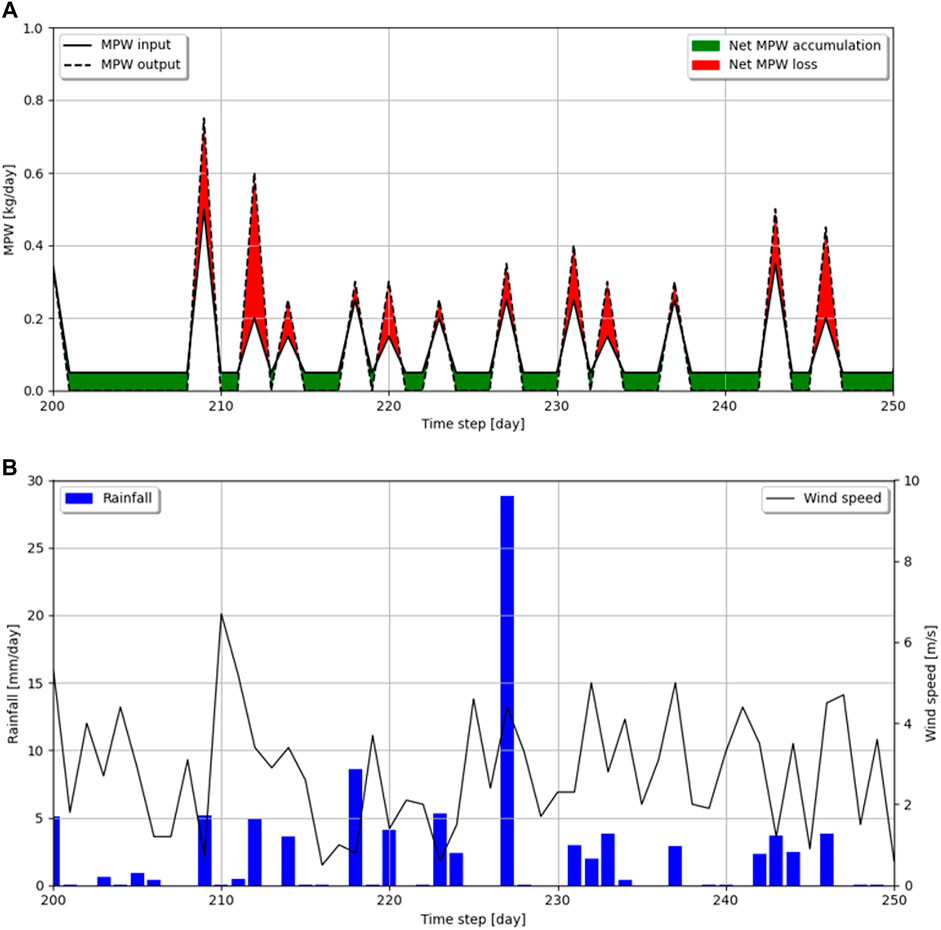
FIGURE 7. (A) The in- and output fluxes of mismanaged plastic waste (kg/day) modelled for the urban grid cell at latitude 21 and longitude 9 (indicated with red box A in Figure 5) for the period day 200 to 250 in the model application. A net accumulation of mismanaged plastic waste (green shading) occurs when the input flux is larger than the output flux. A net loss of mismanaged plastic waste (red shading) occurs when the input flux is lower than the output flux. (B) Rainfall (mm/day) and winds speeds (m/s) for the period day 200 to 250 in the model application.

3.2 Plastic transport routes

Apart from simulating the transport and (re)distribution of MPW that has been added to a river basin, the Plastic Pathfinder can also compute the most likely transport directions of MPW within a river basin for a given set of weather conditions. For this, the model registers for each grid cell in the river basin whether the weather conditions trigger MPW transport, and if so, in which direction. This is done for each time step and for each grid cell, the model keeps count of how often MPW transport is forced in each of the eight transport directions (N, NE, E, SE, S, SW, W, NW). By the end of the last time step, each grid cell has obtained a transport direction distribution. These transport direction distributions are shown in a ‘potential plastics routing map’, whereby the width of the MPW transport arrows are linearly proportional to the frequency with which MPW transport was forced in that particular direction.

The potential plastics routing map generated by our model application (Figure 8) demonstrates that in most grid cells, there is one dominant MPW transport direction. For example, in the grid cell at latitude 24 and longitude 21, the weather input conditions most frequently forced MPW transport to the southeast. The forest grid cells have no transport arrows, this is because the weather conditions were never sufficient to exceed either the wind or surface runoff thresholds. Logically, MPW has the highest chance to be transported in the highest frequency transport directions. Consequently, connecting the high frequency transport directions, i.e. the thickest arrows in the potential plastics routing map, provides a first order estimate on the most likely overland transport route(s) of MPW on a river basin scale.

FIGURE 8

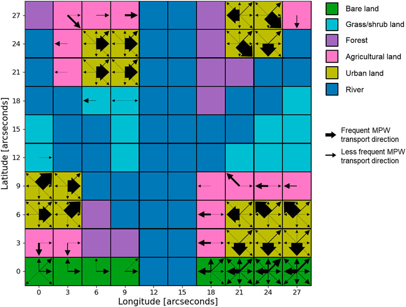
FIGURE 8. Potential plastics routing map that was generated in the model application. Arrows indicate the MPW transport directions that occurred as a result of the terrain characteristics, thresholds, and weather conditions used in the model application described in this study. The width of the arrow is linearly proportional to the frequency with which MPW was transported in that particular direction.

4 Discussion

4.1 Next steps

4.1.1 Model calibration and validation

The Plastic Pathfinder is the first explicit spatiotemporal framework that models the transport of macroplastics in terrestrial environments. However, there are still many uncertainties associated with the accuracy of the model parameterisation, because data are scarce. The current version of the Plastic Pathfinder model uses one threshold for all types of plastic waste. The effect of this assumption on the modelled versus actual plastic accumulation depends on whether the threshold values that were used are an over- or an underestimation. If the thresholds are an overestimation, then the modelled plastic accumulation is likely to be slightly overestimated as well. On the other hand, if the thresholds are an underestimation, then the modelled plastic accumulation is likely to be slightly underestimated as well. Therefore, the next important step is to empirically determine the mobilisation and transport thresholds. For example, physical experiments (e.g., on artificial hillslopes) can elucidate under which wind and surface runoff conditions different types of macroplastics are mobilised and transported over terrains with varying slopes and land uses. Such experiments would offer valuable insights on the mobilisation and transport thresholds of different types of plastic waste (e.g., size, shape, density, wet/dry, etc.) (Schwarz et al., 2019). Moreover, from these experiments the relation between wind speed and plastic transport speed, and surface runoff intensity and plastic transport speed can be explored. These velocities can be used to estimate the travel time of plastics through the terrestrial environment and thereby improve our estimates on the amount of land based MPW that reaches the river, and subsequently the ocean.

Once the Plastic Pathfinder contains empirically proven mobilisation and transport thresholds, the model predictions would ideally be calibrated and validated with observational data. The modelled macroplastic waste distribution on land can be compared with actual macroplastic distribution data; quantified by e.g., field plastic collection efforts (van Emmerik et al., 2020), citizen litter collection projects (Syberg et al., 2020), or optical satellite data (Biermann et al., 2020). We anticipate that future collaborations with field collection and monitoring projects allow for a fast and robust calibration of the Plastic Pathfinder and improve the validity of its predicted MPW transport and fate in river basins.

4.1.2 Future recommendations

The plastic transport simulated by the Plastic Pathfinder is based on the concept of driving forces that need to overcome thresholds. Although this concept appears capable of providing first order predictions on the mobilisation and transport of plastics over land, we would like to make some recommendations for future research. For example, to explore the possibility of a more probabilistic modelling approach (Kooi and Koelmans, 2019), whereby the chance of plastic transport under certain weather conditions is considered. In addition, previous studies have shown that different types of macroplastics have different transport modes (Schwarz et al., 2019). Therefore, we recommend to implement, as soon as they are available, plastic type specific mobilisation and transport thresholds that reflect the differences in mobility and transportability of different types of plastics.

Although the plastic mobilisation and transport thresholds provide information on when (i.e., under which weather conditions) plastics will move, they do not specify how far the plastics will be moved. In the current version of the Plastic Pathfinder the displacement of plastics is restricted to one grid cell per time step, which is acceptable as long as a positive correlation exists between the values of the thresholds and the grid size. Up to date, the travel distance of plastics over land has only been studied for (airborne) microplastics (Allen et al., 2019). We strongly recommend future fundamental research on the relation between wind speed and plastic transport speed and, similarly, between surface runoff fluxes and plastic transport speed.

Moreover, the spatial model resolution determines the degree of detail regarding landscape features. A low spatial model resolution means that small scale barriers that could obstruct the transport of plastic waste are, unjustly, not taken into account. For example, the spatial resolution of the topography map determines whether small height differences, such as dikes, are included. The resolution of the land use map determines the amount of detail that can be captured within for example urban areas to distinguish between roads, buildings, city parks, etc. In addition, the height of grass and shrubs, the height of crops, vegetated waterways, the density of riverbank vegetation or trees in forests, are all landscape characteristics that likely influence the transport and entrapment of plastics. We challenge future research to find a balance between incorporating small scale landscape features and covering an entire river basin.

Finally, we advocate for an all-encompassing model that includes the terrestrial and freshwater environment. This can be achieved by coupling the Plastic Pathfinder with a river plastic transport model, for example with the model developed by Newbould et al. (2021). The river entry points predicted by the Plastic Pathfinder will form this link as they deliver information on where, when and how much plastic waste leaks from land into the river system. This will allow for genuine estimates on how much of the generated land-based plastic waste actually reaches the oceans via rivers.

4.2 The Plastic Pathfinder – an innovative tool

The Plastic Pathfinder is the first model to simulate the transport and accumulation of macroplastic waste over land. Without a fundamental understanding of the MPW transport and retention mechanism in terrestrial systems, the global plastic mass budget cannot be solved (Stephens, 2020; Hoellein and Rochman, 2021). Our model generates potentially high resolution MPW distribution maps, which provide insights on the mechanisms that control the (re)distribution and fate of MPW on land. Moreover, the Plastic Pathfinder identifies the main river entry points of MPW, the locations where terrestrial pollution meets freshwater pollution. With this, the input conditions for riverine plastic transport models can be fine-tuned, which in turn will lead to improved estimates on riverine plastic transport, retention, and emissions to the ocean.

Alongside its scientific significance, the Plastic Pathfinder has a societal relevance as well, as it can provide guidance on the prioritisation of plastic pollution prevention, mitigation and reduction strategies. By knowing when and where plastics on land accumulate and which transport routes they take, targeted clean-up and entrapment strategies can be developed. The removal of plastics from the natural environment is a matter of great urgency, because plastic waste poses serious threats to species health and human livelihood in general (van Emmerik and Schwarz, 2019; Windsor et al., 2019; Bucci et al., 2020; Everaert et al., 2020).

Data availability statement

The original contributions presented in the study are included in the article/Supplementary Material, further inquiries can be directed to the corresponding author. https://doi.org/10.5281/zenodo.6470410.

Author contributions

Conceptualisation: YM, TE; Methodology: YM, TE; Software: YM; Validation: YM, TE; Formal analysis: YM, TE, MK, CL; Investigation: YM; Data curation: YM; Writing–original draft: YM; Writing–review and editing: YM, TE, MK, CL, HN; Visualisation: YM; Supervision: TE, HN; Project administration: YM; Funding acquisition: TE. All authors read and approved the final manuscript.

Funding

The work of TE is part of the Veni research programme The River Plastic Monitoring Project with project number 18211, which is (partly) financed by the Dutch Research Council (NWO). CL acknowledges financial support from the Swiss National Science Foundation under grant 174124. HN received funding through the European Research Council (ERC-CoG Grant No. 772923, project VORTEX).

Conflict of interest

The authors declare that the research was conducted in the absence of any commercial or financial relationships that could be construed as a potential conflict of interest.

Publisher’s note

All claims expressed in this article are solely those of the authors and do not necessarily represent those of their affiliated organizations, or those of the publisher, the editors and the reviewers. Any product that may be evaluated in this article, or claim that may be made by its manufacturer, is not guaranteed or endorsed by the publisher.

Supplementary material

The Supplementary Material for this article can be found online at: https://www.frontiersin.org/articles/10.3389/fenvs.2022.979685/full#supplementary-material

References

Allen, S., Allen, D., Phoenix, V. R., Le Roux, G., Jiménez, P. D., Simonneau, A., et al. (2019). Author Correction: Atmospheric transport and deposition of microplastics in a remote mountain catchment. Nat. Geosci. 12 (8), 679. doi:10.1038/s41561-019-0409-4

CrossRef Full Text | Google Scholar

Anaconda Software Distribution (2016). Computer software. Vers. 2-2.4.0. Available at: https://anaconda.com.

Google Scholar

Barboza, L. G. A., Cózar, A., Gimenez, B. C. G., Barros, T. L., Kershaw, P. J., and Guilhermino, L. (2019). Macroplastics pollution in the marine environment. London: World Seas: an Environmental Evaluation, 305–328. doi:10.1016/b978-0-12-805052-1.00019-x

CrossRef Full Text | Google Scholar

Bartholomé, E., and Belward, A. S. (2005). GLC2000: A new approach to global land cover mapping from Earth observation data. Int. J. Remote Sens. 26 (9), 1959–1977. doi:10.1080/01431160412331291297

CrossRef Full Text | Google Scholar

Biermann, L., Clewley, D., Martinez-Vicente, V., and Topouzelis, K. (2020). Finding plastic patches in coastal waters using optical satellite data. Sci. Rep. 10 (1), 1–10. [online]. doi:10.1038/s41598-020-62298-z

PubMed Abstract | CrossRef Full Text | Google Scholar

Bucci, K., Tulio, M., and Rochman, C. M. (2020). What is known and unknown about the effects of plastic pollution: A meta‐analysis and systematic review. Ecol. Appl. 30 (2), e02044. doi:10.1002/eap.2044

PubMed Abstract | CrossRef Full Text | Google Scholar

dataplatform.knmi.nl (2000). Frequency tables 1981-2000 - KNMI data Platform. [online] Available at: https://dataplatform.knmi.nl/dataset/frequentietabellen-1981-2000-v1-0.

Google Scholar

Delandmeter, P., and van Sebille, E. (2019). The parcels v2.0 Lagrangian framework: New field interpolation schemes. Geosci. Model Dev. 12 (8), 3571–3584. doi:10.5194/gmd-12-3571-2019

CrossRef Full Text | Google Scholar

Everaert, G., De Rijcke, M., Lonneville, B., Janssen, C. R., Backhaus, T., Mees, J., et al. (2020). Risks of floating microplastic in the global ocean. Environ. Pollut. 267, 115499. doi:10.1016/j.envpol.2020.115499

PubMed Abstract | CrossRef Full Text | Google Scholar

Geyer, R., Jambeck, J. R., and Law, K. L. (2017). Production, use, and fate of all plastics ever made. Sci. Adv. 33 (7), e1700782. doi:10.1126/sciadv.1700782

PubMed Abstract | CrossRef Full Text | Google Scholar

Ghiggi, G., Humphrey, V., Seneviratne, S. I., and Gudmundsson, L. (2019). Grun: An observation-based global gridded runoff dataset from 1902 to 2014. Earth Syst. Sci. Data 11 (4), 1655–1674. doi:10.5194/essd-11-1655-2019

CrossRef Full Text | Google Scholar

Global Wind Atlas (2019). Global wind Atlas. [online] Available at: https://globalwindatlas.info/.

Google Scholar

Goel, M. K. (2011). Runoff coefficient. Dordrecht: Encyclopedia of Earth Sciences Series, 952–953. doi:10.1007/978-90-481-2642-2_456

CrossRef Full Text | Google Scholar

Hardesty, B. D., Harari, J., Isobe, A., Lebreton, L., Maximenko, N., Potemra, J., et al. (2017). Using numerical model simulations to improve the understanding of micro-plastic distribution and pathways in the marine environment. Front. Mar. Sci. 4. [online] 4. doi:10.3389/fmars.2017.00030

CrossRef Full Text | Google Scholar

Hoellein, T. J., and Rochman, C. M. (2021). The ‘plastic cycle’: A watershed‐scale model of plastic pools and fluxes. Front. Ecol. Environ. 19 (3), 176–183. doi:10.1002/fee.2294

CrossRef Full Text | Google Scholar

Jenson, S. K., and Domingue, J. O. (1988). Extracting topographic structure from digital elevation data for geographic information system analysis. Am. Soc. Photogrammetry Remote Sens. 54 (11), 1593–1600.

Google Scholar

Karamage, F., Zhang, C., Fang, X., Liu, T., Ndayisaba, F., Nahayo, L., et al. (2017). Modeling rainfall-runoff Response to land use and land cover change in Rwanda (1990–2016). Water 9 (2), 147. doi:10.3390/w9020147

CrossRef Full Text | Google Scholar

Kooi, M., and Koelmans, A. A. (2019). Simplifying microplastic via continuous probability distributions for size, shape, and density. Environ. Sci. Technol. Lett. 6 (9), 551–557. doi:10.1021/acs.estlett.9b00379

CrossRef Full Text | Google Scholar

Land Cover CCI Product User Guide Version 2.0 (2017). Document ref: CCI-LC-PUGV2 deliverable ref: D3.3. VERSION: 2.0. [online] Available at: http://maps.elie.ucl.ac.be/CCI/viewer/download/ESACCI-LC-Ph2-PUGv2_2.0.pdf.

Google Scholar

Lau, W. W. Y., Shiran, Y., Bailey, R. M., Cook, E., Stuchtey, M. R., Koskella, J., et al. (2020). Evaluating scenarios toward zero plastic pollution. Science 369 (6510), 9475. [online]. doi:10.1126/science.aba9475

PubMed Abstract | CrossRef Full Text | Google Scholar

Lebreton, L., and Andrady, A. (2019). Future scenarios of global plastic waste generation and disposal. Palgrave Commun. 5 (1), 6. doi:10.1057/s41599-018-0212-7

CrossRef Full Text | Google Scholar

Lebreton, L. C.-M. , Greer, S. D., and Borrero, J. C. (2012). Numerical modelling of floating debris in the world’s oceans. Mar. Pollut. Bull. 64 (3), 653–661. doi:10.1016/j.marpolbul.2011.10.027

PubMed Abstract | CrossRef Full Text | Google Scholar

Lebreton, L. C. M., van der Zwet, J., Damsteeg, J.-W., Slat, B., Andrady, A., and Reisser, J. (2017). River plastic emissions to the world’s oceans. Nat. Commun. 8 (15611), 15611. [online]. doi:10.1038/ncomms15611

PubMed Abstract | CrossRef Full Text | Google Scholar

Lehner, B., Verdin, K., and Jarvis, A. (2008). New global hydrography derived from spaceborne elevation data. Eos Trans. AGU. 89 (10), 93. doi:10.1029/2008eo100001

CrossRef Full Text | Google Scholar

Materić, D., Kasper-Giebl, A., Kau, D., Anten, M., Greilinger, M., Ludewig, E., et al. (2020). Micro- and nanoplastics in alpine snow: A new method for chemical identification and (Semi)Quantification in the nanogram range. Environ. Sci. Technol. 54 (4), 2353–2359. doi:10.1021/acs.est.9b07540

PubMed Abstract | CrossRef Full Text | Google Scholar

Maximenko, N., Hafner, J., and Niiler, P. (2012). Pathways of marine debris derived from trajectories of Lagrangian drifters. Mar. Pollut. Bull. 65 (1-3), 51–62. doi:10.1016/j.marpolbul.2011.04.016

PubMed Abstract | CrossRef Full Text | Google Scholar

Meijer, L. J. J., van Emmerik, T., van der Ent, R., Schmidt, C., and Lebreton, L. (2021). More than 1000 rivers account for 80% of global riverine plastic emissions into the ocean. Sci. Adv. 7 (18), eaaz5803. doi:10.1126/sciadv.aaz5803

PubMed Abstract | CrossRef Full Text | Google Scholar

Met Office (2010). National meteorological library and archive fact sheet 6 – the Beaufort scale. [online]. Available at: https://web.archive.org/web/20121002134429/http://www.metoffice.gov.uk/media/pdf/4/4/Fact_Sheet_No._6_-_Beaufort_Scale.pdf.

Google Scholar

Newbould, R. A., Powell, D. M., and Whelan, M. J. (2021). Macroplastic debris transfer in rivers: A travel distance approach. Front. Water 3. doi:10.3389/frwa.2021.724596

CrossRef Full Text | Google Scholar

Njeru, J. (2006). The urban political ecology of plastic bag waste problem in Nairobi, Kenya. Geoforum 37 (6), 1046–1058. doi:10.1016/j.geoforum.2006.03.003

CrossRef Full Text | Google Scholar

Onink, V., Jongedijk, C. E., Hoffman, M. J., van Sebille, E., and Laufkötter, C. (2021). Global simulations of marine plastic transport show plastic trapping in coastal zones. Environ. Res. Lett. 16 (6), 064053. doi:10.1088/1748-9326/abecbd

CrossRef Full Text | Google Scholar

Ribeiro, F., Okoffo, E. D., O’Brien, J. W., Fraissinet-Tachet, S., O’Brien, S., Gallen, M., et al. (2020). Correction to quantitative analysis of selected plastics in high-commercial-value Australian seafood by pyrolysis Gas chromatography mass spectrometry. Environ. Sci. Technol. 54 (20), 13364. doi:10.1021/acs.est.0c05885

PubMed Abstract | CrossRef Full Text | Google Scholar

Schmidt, C., Krauth, T., and Wagner, S. (2017). Export of plastic debris by rivers into the sea. Environ. Sci. Technol. 51 (21), 12246–12253. doi:10.1021/acs.est.7b02368

PubMed Abstract | CrossRef Full Text | Google Scholar

Schwarz, A. E., Ligthart, T. N., Boukris, E., and van Harmelen, T. (2019). Sources, transport, and accumulation of different types of plastic litter in aquatic environments: A review study. Mar. Pollut. Bull. 143, 92–100. doi:10.1016/j.marpolbul.2019.04.029

PubMed Abstract | CrossRef Full Text | Google Scholar

Shields, A. (1936). Application of similarity principles and turbulence research to bed-load movement. CalTech library. [online] Available at: https://repository.tudelft.nl/islandora/object/uuid%3Aa66ea380-ffa3-449b-b59f-38a35b2c6658.

Google Scholar

Sigler, M. (2014). The effects of plastic pollution on aquatic wildlife: Current situations and future solutions. Water Air Soil Pollut. 225 (11), 2184. doi:10.1007/s11270-014-2184-6

CrossRef Full Text | Google Scholar

Stephens, M. (2020). The search for the missing plastic. Phys. World 33 (5), 40–44. doi:10.1088/2058-7058/33/5/30

CrossRef Full Text | Google Scholar

Syberg, K., Palmqvist, A., Khan, F. R., Strand, J., Vollertsen, J., Clausen, L. P. W., et al. (2020). A nationwide assessment of plastic pollution in the Danish realm using citizen science. Sci. Rep. 10 (1), 17773–17811. [online] 10. doi:10.1038/s41598-020-74768-5

PubMed Abstract | CrossRef Full Text | Google Scholar

Tramoy, R., Gasperi, J., Colasse, L., Silvestre, M., Dubois, P., Noûs, C., et al. (2020). Transfer dynamics of macroplastics in estuaries – new insights from the seine estuary: Part 2. Short-Term dynamics based on GPS-trackers. Mar. Pollut. Bull. 160, 111566. doi:10.1016/j.marpolbul.2020.111566

PubMed Abstract | CrossRef Full Text | Google Scholar

van Emmerik, T., Loozen, M., van Oeveren, K., Buschman, F., and Prinsen, G. (2019). Riverine plastic emission from Jakarta into the ocean. Environ. Res. Lett. 14 (8), 084033. doi:10.1088/1748-9326/ab30e8

CrossRef Full Text | Google Scholar

van Emmerik, T., Mellink, Y., Hauk, R., Waldschläger, K., and Schreyers, L. (2022). Rivers as plastic reservoirs. Front. Water 3. doi:10.3389/frwa.2021.786936

CrossRef Full Text | Google Scholar

van Emmerik, T., and Schwarz, A. (2019). Plastic debris in rivers. WIREs Water 7 (1). doi:10.1002/wat2.1398

CrossRef Full Text | Google Scholar

van Emmerik, T., Vriend, P., and Roebroek, J. (2020). An evaluation of the River-OSPAR method for quantifying macrolitter on Dutch riverbanks. Wageningen: Wageningen University. [online] research.wur.nlAvailable at: https://research.wur.nl/en/publications/an-evaluation-of-the-river-ospar-method-for-quantifying-macrolitt.

Google Scholar

van Sebille, E., England, M. H., and Froyland, G. (2012). Origin, dynamics and evolution of ocean garbage patches from observed surface drifters. Environ. Res. Lett. 7 (4), 044040. doi:10.1088/1748-9326/7/4/044040

CrossRef Full Text | Google Scholar

Vethaak, A. D., and Leslie, H. A. (2016). Plastic debris is a human health issue. Environ. Sci. Technol. 50 (13), 6825–6826. doi:10.1021/acs.est.6b02569

PubMed Abstract | CrossRef Full Text | Google Scholar

Wayman, C., and Niemann, H. (2021). The fate of plastic in the ocean environment – A minireview. Environ. Sci. Process. Impacts 23 (2), 198–212. doi:10.1039/d0em00446d

PubMed Abstract | CrossRef Full Text | Google Scholar

Windsor, F. M., Durance, I., Horton, A. A., Thompson, R. C., Tyler, C. R., and Ormerod, S. J. (2019). A catchment‐scale perspective of plastic pollution. Glob. Chang. Biol. 25 (4), 1207–1221. doi:10.1111/gcb.14572

PubMed Abstract | CrossRef Full Text | Google Scholar

Yeo, S.-S. , and Hsuan, Y. G. (2010). Evaluation of creep behavior of high density polyethylene and polyethylene-terephthalate geogrids. Geotext. Geomembranes 28 (5), 409–421. doi:10.1016/j.geotexmem.2009.12.003

CrossRef Full Text | Google Scholar