Water quality monitoring and assessment based on cruise monitoring, remote sensing, and deep learning: A case study of Qingcaosha Reservoir

Accurate monitoring and assessment of the environmental state, as a prerequisite for improved action, is valuable and necessary because of the growing number of environmental problems that have harmful effects on natural systems and human society. This study developed an integrated novel framework containing three modules remote sensing technology (RST), cruise monitoring technology (CMT), and deep learning to achieve a robust performance for environmental monitoring and the subsequent assessment. The deep neural network (DNN), a type of deep learning, can adapt and take advantage of the big data platform effectively provided by RST and CMT to obtain more accurate and improved monitoring results. It was proved by our case study in the Qingcaosha Reservoir (QCSR) that DNN showed a more robust performance (R² = 0.89 for pH, R² = 0.77 for DO, R² = 0.86 for conductivity, and R² = 0.95 for backscattered particles) compared to the traditional machine learning, including multiple linear regression, support vector regression, and random forest regression. Based on the monitoring results, the water quality assessment of QCSR was achieved by applying a deep learning algorithm called improved deep embedding clustering. Deep clustering analysis enables the scientific delineation of joint control regions and determines the characteristic factors of each area. This study presents the high value of the framework with a core of big data mining for environmental monitoring and follow-up assessment in a manner of high frequency, multidimensionality, and deep hierarchy.

1 Introduction

A growing population and climate change along with land use changes are increasing pollutant loads into freshwater ecosystems, making clean water an increasingly critical issue worldwide Sagan et al. (2020). As one of the indispensable foundations of clean water management, developing an economical, accurate, and practical water quality monitoring and assessing system has become unavoidable to scientists, policymakers, and environmental resource managers.

The traditional and widely applied water quality monitoring is point-based, placing a fixed site of varying density and dispersion in the area to measure the water quality within a given time series. However, limited research resources such as staff, time, equipment, money, and accessibility become a challenge. Thus, the spatial interpolation method was conducted to estimate water quality by limited monitoring points Li and Heap (2014). This method required a massive decentralized monitoring point across the study area, which is also subjected to limited research resources Lee et al. (2012).

With the significant development of sensors, cruise monitoring technology (CMT) has proven to be more effective for extracting environment-related parameters compared to point-based monitoring Holbach et al. (2014). It relies on a multisensor probe to record the water quality data as well as consecutive geographic information along the cruise route. Although CMT makes progress in monitoring compared to the point-based method because it can collect a large amount of in situ measurement data in a certain period of time, a route design is still necessary since the geographic information is a key parameter to spatial interpolation modeling.

In recent years, remote sensing technology (RST) has developed rapidly and played a significant role in the data collection and analysis of different Earth resources Feyisa et al. (2014). The data collected by RST are area-based since RST can scan the objective area directly. The status of water quality in a broader space is obtained according to an inversion model established using the in situ monitoring data (i.e., water quality parameters) and corresponding RST image data Yuan et al. (2020). According to the interaction with light, water-quality parameters can be categorized into optical parameters (i.e., chlorophyll-a and turbidity) and nonoptical parameters (i.e., dissolved oxygen); it should be noted that most of the studies have focused on optical parameters, and the detection accuracy for nonoptical parameters is not high Hassan et al. (2021). Specific internal correlations between spectral information and nonoptical parameters are very complex and challenging to find due to the absence of direct optical properties Niu et al. (2021). Therefore, data-driven machine learning has become an indispensable tool for finding this complex correlation Zhong et al. (2021) Sagan et al. (2020). In earlier studies, linear approaches such as multiple linear regression (MLR), partial least squares (PLSs), and genetic algorithms (GAs) were popular Ortiz-Casas and Peña-Martinez (1989); Stork and Autrey (2005); Zhan et al. (2003). Although linear models showed some degree of accuracy and feasibility, the nonlinear relationship between the in situ measured data and RST data makes the linear models less reliable in interpreting information from RST Chang et al. (2015). With the development of machine learning, several nonlinear approaches such as support vector regression (SVR), random forest regression (RFR), and gradient boosting decision tree (GBDT) have been developed and applied by many scientists to capture complex statistical relationships between RST and measured water quality parameters in recent years Kim et al. (2014); Forkuor et al. (2017); Abdel-Rahman et al. (2013). With the advances in algorithm development and computing power, the drawbacks of traditional machine learning become apparent, while deep learning, with its powerful big data processing capabilities, is receiving more attention. In our framework, deep neural networks (DNNs), one type of deep learning, were selected as a tool to approximate the complex nonlinear relationship between measured water quality parameters and RST observations through multilayer perception Marçais and de Dreuzy (2017).

It is important to note that the performance of deep learning methods is particularly dependent on a large number of training samples, which is difficult to obtain in real-world scenarios Sagan et al. (2020). The CMT mentioned earlier can significantly increase the speed of acquiring training samples, thus providing a sufficient database for deep learning RST inversion model building. On the other hand, RST, to a certain degree, liberates CMT from dependence on route design since geographic information is not involved in the inversion modeling.

As an important part of the water monitoring project, a representative and reliable assessment of water quality is necessary because of the spatial and temporal variability of water parameters Simeonov et al. (2003). The conventional methods for assessing the quality of water bodies are the single-factor assessment method, water quality grading method, and comprehensive pollution index method. These methods play an active role in the assessment process of water quality. However, the single-factor assessment method does not fully describe the overall water quality when there are multiple impairments. The water quality grading method ignores the influence of extreme contributing factors (maximum and minimum pollutant parameter values), making it difficult to assess the overall water quality conditions between sites when extreme conditions occur. The calculation result of the comprehensive pollution index method is a relative value and cannot indicate the specific water quality classification Ji et al. (2016). In particular, when faced with the huge and complex matrix of water quality attributes formed by the establishment of a big data platform like this study, making a meaningful water quality assessment is often difficult Singh et al. (2005). A cluster analysis can be applied to interpret these complex data matrices to help understand the water quality and ecological status of the studied systems, identifying the possible resources and finding rapid solutions to pollution problems by grouping the data so that similar elements are assigned to the same group and different elements are assigned to different ones Vo-Van et al. (2020); Simeonov et al. (2003). Additionally, considering that deep clustering is more effective at analyzing big data than traditional clustering methods Guo et al. (2017), such as K-means and C-means, an advanced deep learning clustering algorithm, improved deep embedded clustering (IDEC), was used for the water quality assessment in this study.

The aim of this study is to develop a novel framework with a core of big data mining, integrating (1) CMT data from multisensor monitoring systems, 2) RST information from the satellites, and 3) deep learning for rapid and effective overall water quality evaluation and the follow-up assessment of the environmental situation. This novel framework was applied in the Qingcaosha Reservoir (QCSR), located in Shanghai, to prove its reasonability and reliability.

2 Materials and methods

To achieve a robust performance in water quality monitoring and assessment, the framework integrates the following three modularized parts: RST, CMT, and deep learning. The DNN model is responsible for efficient water quality monitoring on a big data platform created by CMT and RST, while the IDEC model is used for further assessment based on the previous monitoring results (Figure 1A). A sampling activity in QCSR (Supplementary Figure S1) was implemented to validate the performance of the framework. QCSR is one of the largest tidal reservoirs around the world. It is located in the middle of the Yangtze River Estuary (31.42–31.49N, 121.55–121.71E), and is the new largest drinking water supply for about 12 million Shanghai residents Liu et al. (2016a) since 2010 (Figure 2). The reservoir is long and narrow with a surface area of approximately 70 km² and an average depth of 2.7 m Liu et al. (2016b).

FIGURE 1

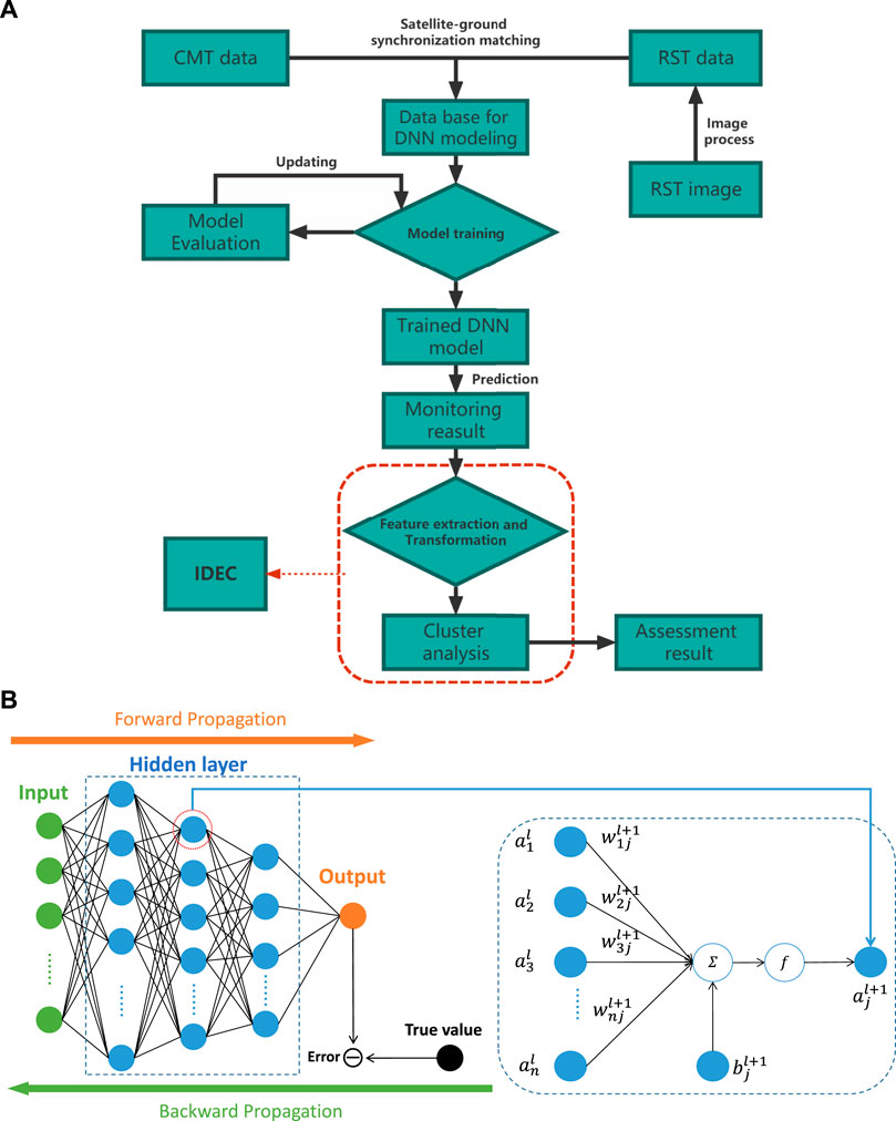
FIGURE 1. Schematic illustration of (A) the novel framework and (B) the architecture of DNN.

FIGURE 2

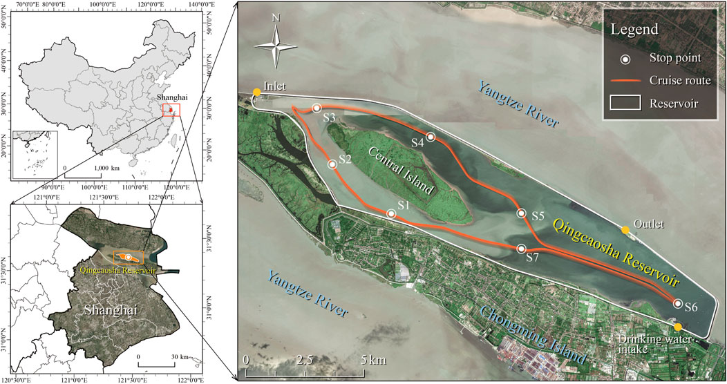
FIGURE 2. Study area and cruise route.

2.1 Remote sensing module

Sentinel-2 is an Earth observation satellite designed to systematically deliver optical imagery at high spatial resolution (10, 20, and 60m) over land and waters Drusch et al. (2012) (Supplementary Table S2). Due to its relatively high resolution and free accessibility, Sentinel-2 is widely used in environmental research. Its multi-spectral instrument (MSI) acquires 13 spectral bands from 440 nm to 2,200 nm. The image of Sentinel-2 on 19 January 2020 (the same day as the CMT in situ measurement) was downloaded from the official website of the U.S. Geological Survey (https://earthexplorer.usgs.gov/). The level-1C data product was selected in this study and this series of data has been radiometrically and geometrically corrected (including orthorectification).

RST image is processed in order of radiometric calibration, atmospheric correction, RST image fusion, and research area clipping to finish the conversion from images to spectral values (Figure 1A). One conventional atmospheric correction algorithm, Fast Line-of-Sight Atmospheric Analysis of Hypercubes (FLAASH) was set as an atmospheric correction algorithm in this study Buma and Lee (2020). The specific RST parameters set, including ground elevation, atmospheric model, aerosol retrieval, and water retrieval, were found in the files alongside their respective multispectral images. The RST images (not including bands 1, 9, and 10) were resampled to 10 m by the Gram-Schmidt pan sharpening method (Supplementary Material), one of the most widely used high-quality methods for RST image fusion Zhang et al. (2019). All of the RST data processing could be conducted using the packaged functions in ENVI^Ⓡ. The RST data were processed by Z-score normalization (Supplementary Material) before being input to the models. It should be noted that when new data are collected, the normalization part performs a new normalization of the overall data set (containing the previous data set and the new data set) for the training model.

2.2 Cruise monitoring module

Cruise monitoring with multiple sensors is conducted by BioFish in this study. It is an aquatic cruise monitoring system that is equipped with multisensors (Supplementary Table S1) and connected to a ship by a data transmission cable Udy et al. (2005). The data of water quality parameters were recorded in real-time with GPS longitudinal and latitudinal positions. In this study, the BioFish swam 10 cm below the water surface. One optical parameter, backscattered particles (BPs, similar to turbidity, measured by a beam attenuation probe to estimate water clarity) (Supplementary Material), and three nonoptical parameters, including electrical conductivity (El.cond), pH value, and dissolved oxygen (DO), are selected to validate the performance of the framework.

Due to the limitations of power supply, equipment, time, and accessibility, the in situ measuring in QCSR was finished within 1 day and the running time was 5 hours. The cruise route is shown in Figure 2, aiming to cover as much of the study area as possible. S1 is the start and end point of the cruise route. Seven stopping points were designed for (S1–S7, see Figure 2) the BioFish calibration with the YSL ProDSS to ensure the accuracy of the data. An overview of the data collected by BioFish in QCSR is displayed in Table 1. The BioFish data were processed by Z-score normalization (Supplementary Material) and satellite–ground synchronization matching (Supplementary Figure S2) before being input into the models (Figure 1A). It should be noted that the normalization section renormalizes the new overall dataset when new data are collected.

TABLE 1

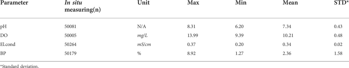
TABLE 1. Summary statistics of the BioFish data.

Since the high sampling density of BioFish means that multiple BioFish sampling points can be found randomly in a pixel block of size 10 m × 10 m, determining the BioFish sampling points within the same pixel block and deriving their representative values are required. The first step is to specify the spatial information of all BioFish sampling points and pixel grid centroids. The geodesic distance Shamai and Kimmel (2017) between the pixel grid centroid and the BioFish sampling point can be calculated by the Python package geopy, with an ellipsoidal model, WGS-84. Then, the pixel grid corresponding to the BioFish sampling point can be extracted by finding the shortest geodesic distance between them. The next step is calculating the representative values of BioFish measurements within each pixel block by the arithmetic mean (AM).

2.3 Water quality monitoring model

In this section, deep neural networks and three traditional machine learning models are used to find the relationship between RST and CMT and compare their performance, respectively.

2.3.1 Deep neural network

The deep neural network (DNN) is the basic form of deep learning and one of the most efficient and powerful tools to model complex nonlinear relationships Rolnick and Tegmark (2018). As the left side of Figure 1B shows, DNN is a connectionist system with multiple hidden layers between the input and output layers. Each hidden layer contains multiple neurons, called nodes. Any node in the lth layer must be connected to any node in the l + 1st layer, and the following equation indicates the nonlinear relationship between the DNN layers shown on the right side of Figure 1B:

${\text{a}}_j^{l+1}=f\left(\sum _{i=1}^n{a}_i^l{w}_{ij}^l+b_j^l\right),$

where $a_i^l$ is the activation value of the ith node in the lth layer, $a_j^{l+1}$ is the activation value of the jth node in the l + 1st layer,$w_{ij}^{l+1}$is the weight between $a_i^l$ and $a_j^{l+1}$, $b_j^{l+1}$ is the bias value of the jth node in the l + 1st layer, and f (⋅) is the active function.

The training process is shown on the left side of Figure 1B. Forward propagation refers to the calculation and storage of intermediate variables (including outputs) from the input to the output layer. Back propagation refers to the method of calculating the gradient of neural network parameters and updating the parameters depending on the error between the output and true value. For tuning hyperparameters in this study, relu Agarap (2018) was set as the active function and adam as the optimizer of all models. The layer and neural units of models were (256, 256, 256, 256, 256) except El.cond.-spectral value was (256, 256, 256). Additionally, batch size and learning rate were also tuned in a reasonable range.

2.3.2 Multiple linear regression

Linear regression, a typical traditional machine learning model, is a linear approach for estimating the relationship between a dependent variable and one or more independent variables. The case of one independent variable is called simple linear regression; for two or more, the process is called multiple linear regression (MLR) Berger et al. (2017). In this study, the MLR model was built by calling the function in the Python package scikit-learn. The parameter to be tuned in this study was the degree of the polynomial features.

2.3.3 Support vector regression

Support vector regression (SVR) is a traditional supervised machine learning that is applied widely in RST inversion Wagle et al. (2020). The SVR model was also conducted by calling the function in the Python package scikit-learn. The radial basis function was chosen as the kernel of SVR. The parameters that need to be tuned in this study are the regularization parameter and the kernel coefficient.

2.3.4 Random forest regression

Random forest regression (RFR) is a traditional machine learning algorithm for nonlinear regression. It uses an ensemble learning method that combines a large set of regression trees to make a more accurate regression than a single regression tree Kim et al. (2014). The RFR model was implemented by calling the function in the Python package scikit-learn. The n-estimators and random-state need to be tuned.

2.3.5 Evaluation metrics

Evaluating the performance of a model is an essential step before practical application. We split each dataset into a training set and a test set with a ratio of 4:1 and take one at every four intervals as the test data. Several indicators, including the coefficient of determination (R²), root mean square error (RMSE), mean absolute percentage error (MAPE), and median absolute deviation (MAD), were used to evaluate each regression model’s accuracy, stability, and inversion ability (Supplementary Material).

2.4 Water quality assessment model

Improved deep embedded clustering is an unsupervised deep learning algorithm for clustering. The monitoring results obtained from the framework were clustered using IDEC, and points with similar environmental states were grouped based on the combined effect of all measured water quality parameters (pH, DO, BP, and El.cond in this study), thus dividing the entire reservoir into different areas possessing different environmental states. According to the clustering results, each group’s specific water quality characteristics can be understood by analyzing the distribution of each group’s characteristic water quality parameters. This characteristic of each group is the main reason why these measurement points are clustered into the same group, and it can also be described as the characteristic factor of this group.

The structure of IDEC includes an encoder and a decoder network Guo et al. (2017) (Supplementary Figure S3). The encoder network is set as a fully connected multilayer perceptron (MLP) with dimensions 4-125-125-500-10. The decoder network is a mirror of the encoder with dimensions 10-500-125-125-4. relu was set as the active function and adam as the optimizer of all models. The coefficient of cluster loss γ is set to 0.1 and batch size to 256. The convergence threshold δ is set to 0.1%. Also, the update interval T is one iteration. IDCE and CH method was conducted by PyTorch. The number of clusters was determined by the Calinski–harabasz (CH) method Zhao and Fränti (2014).

3 Results

Considering the conceptual merits of the developed framework, we applied the framework to a database of QCSR sampling activity to evaluate its performance on inversion and make the assessment of water quality through clustering results.

3.1 Model performance evaluation

Based on the performance of the regression model for four water quality parameters, several results are achieved.

1) DNN represented the best performance in accuracy and stability compared to the other three algorithms. The results for the model performance are summarized in Table 2. Concerning the inversion of pH, SVR, RFR, and DNN delivered satisfactory results. DNN achieved the highest R² = 0.889 and the lowest RMSE = 0.33, MAPE = 0.52, and MAD = 0.10 that stand for the stability of DNN. As for the DO and El.cond inversion, DNN achieved the highest accuracy with R² = 0.77, 0.86 compared with MLR, SVR, and RFR. In addition, the lowest RMSE (0.49 for DO and 0.38 for El.cond) and MAD (0.06 for DO and 0.06 for El. Cond) demonstrated that DNN has high stability even though the MAPE of DNN is slightly less than that of SVR.

TABLE 2

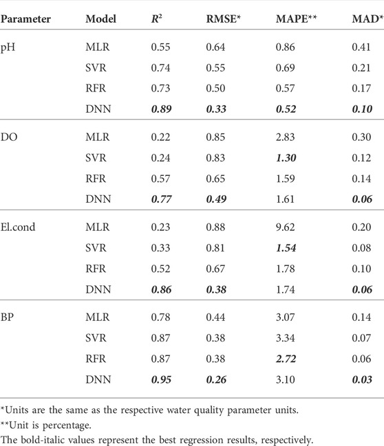
TABLE 2. Results of regression model evaluation.

With respect to the inversion of BP, all models express relatively satisfactory results. In particular, DNN reached a very high accuracy with R² = 0.95 and relatively low RMSE, MAPE, and MAD.

The comparison of predicted values and the measured values on the test set are shown in Figure 3. It is found that the slope of DNN test results (0.90 for pH, 0.67 for DO, 0.82 for El.cond, and 0.92 for BP) is much larger than those of MRL, SVR, and RFR. Therefore, DNN significantly improved the inversion accuracy compared with MLR, SVR, and RFR.

FIGURE 3

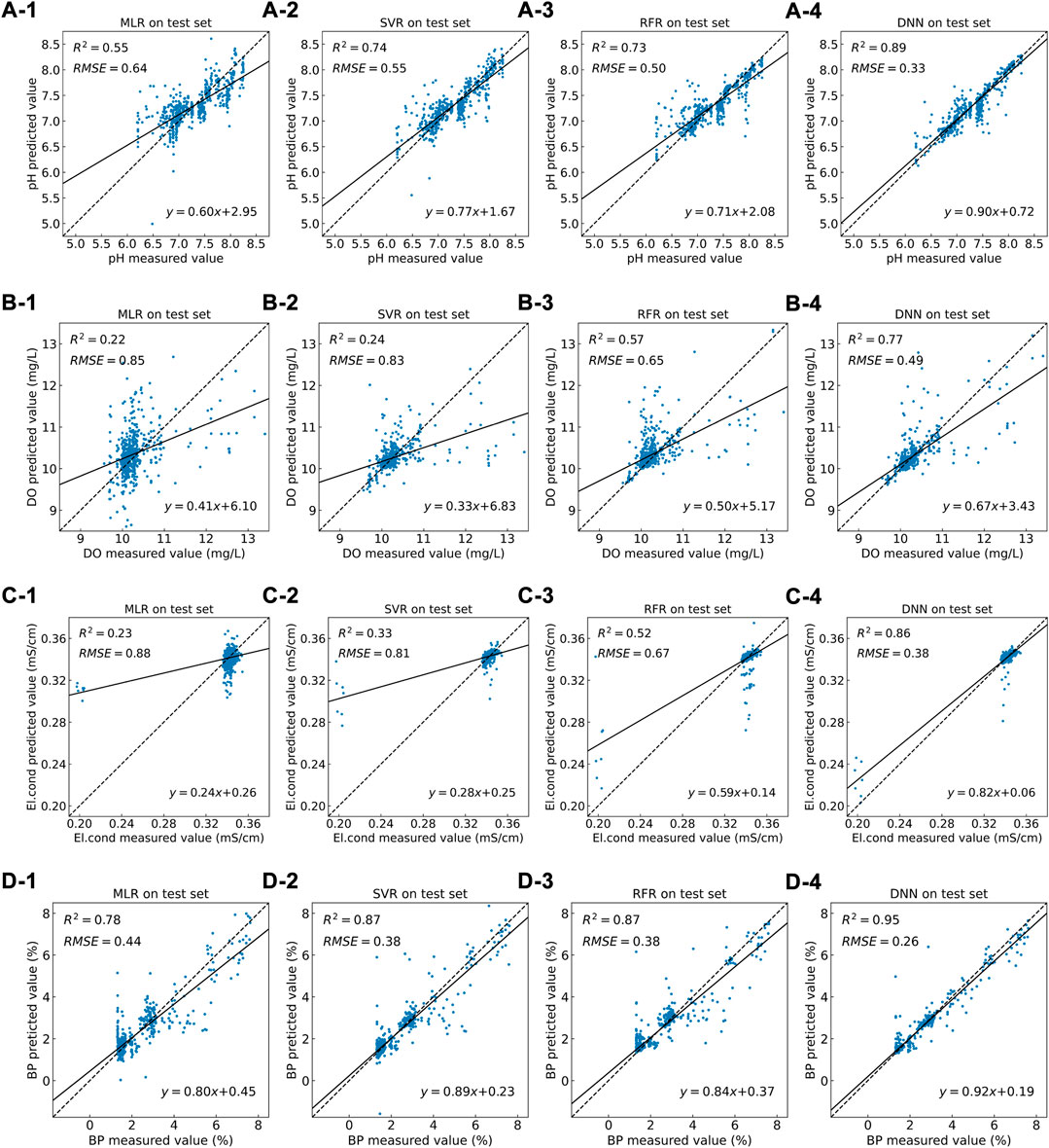
FIGURE 3. Regression model performance evaluation by comparison of the predicted data and measured data on a test set, where (A), (B), (C), and (D) represent the test results of the pH, DO, El.cond, and BP, respectively and (1), (2), (3), and (4) represent the test results of the MLR, SVR, RFR, and DNN, respectively.

2) The performance of each model increases with increasing training data size. We randomly select 0–100% of the data in the original dataset at 10% intervals for training and testing. This process is performed 50 times for each data size, and then the average performance of the model (denoted by R²) and its standard deviation (Supplementary Material) are calculated at each data size. As the training data size increases, the results of each water quality parameter consistently showed an increasing trend of R² (Figure 4). It can be also found that DNN is highly sensitive to training data size. The performance of DNN was not the best among the four models with a small training data size, especially when less than 30% of the training data size was fed. (Figure 4D). When 40% or more of the training data are fed, a critical point is noted, where DNN performance surpasses the other models. In particular, a significant advantage of DNN can be observed as the training data size increases from 50% to 100%. Meanwhile, a more advanced performance of DNN could be expected.

FIGURE 4

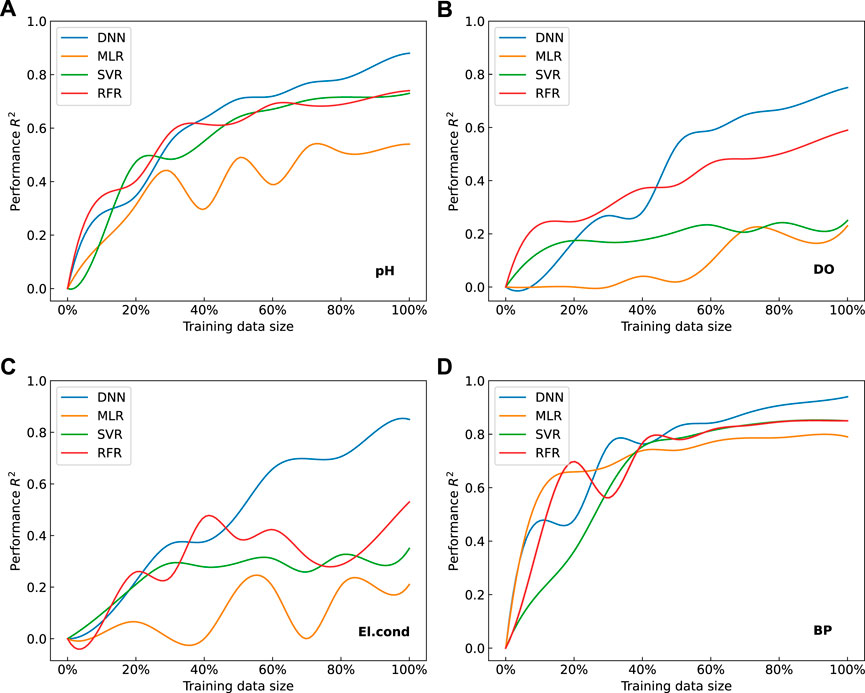
FIGURE 4. Performance of each regression model with increasing training data size, where (A–D) represent the results of the pH, DO, El.cond and BP, respectively.

3.2 Application of the developed framework in QCSR

The concentration heat-maps of each parameter (pH, DO, El.cond, and BP) are shown in Figures 5A–D, respectively. The pH value obtained by the developed framework ranges from 6.2 to 8.9, with a mean value of 7.2. The results reveal spatial difference in that pH value decreases from the head region of QCSR to the tail region (see Figure 5A). The inverted DO ranges from 6.90 mg/L to 14.00 mg/L, with a mean value of 10.30 mg/L. The results show a similar spatial difference as that of pH since the concentration of DO decreases from Figure 5Bthe head region to the tail region, as shown in Figure 5B. Differing from the pH value, a relatively low concentration of DO occurs in the eastern portion of the reservoir, the tail region. The result of El.cond ranges from 0.20 mS/cm to 0.44 mS/cm, with a mean value of 0.34 mS/cm. El.cond observed in the head region is lower than that of the rest area (see Figure 5C). The inverted BP ranges from 0.10 to 10.00%, with a mean value of 2.13%. The results show a similar spatial difference as that of pH since BP decreases from the head to the tail region, as shown in Figure 5D.

FIGURE 5

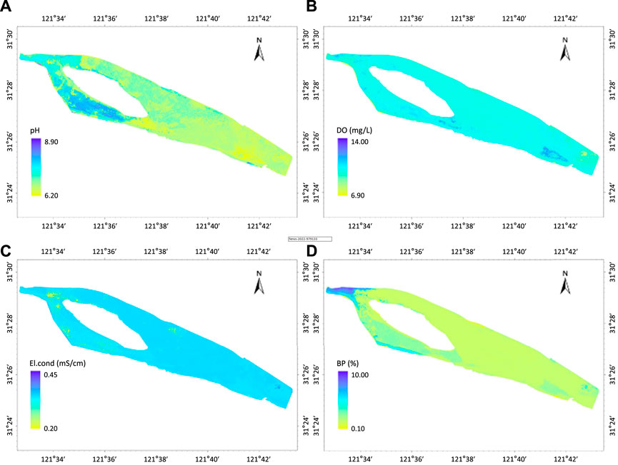
FIGURE 5. Distribution of (A) pH, (B) DO, (C) El.cond, and (D) BP in QCSR based on the framework.

The entire QCSR can be divided into four groups of water bodies by the CH method (Supplementary Material, Figure 4), which are groups I, II, III, and IV. The summary statistics and distributions of each group obtained by IDEC are shown in Table3 and Figure 6. Group I occupied 73.79% of the entire QCSR area. It exhibits characteristics that the values for each parameter are in the middle position compared to others. Group I is dominated from the northeast of the central island to the tail region. The proportions of group II and III water were 4.99 and 3.23%, respectively. Group II is characterized by significantly higher BP values than the other groups and is distributed at the head of the reservoir and on the southern shore of the reservoir. Group III shows a higher DO value compared to other groups and is distributed close to the drinking water intake. Group IV has a higher pH value compared to others, indicating a mildly alkaline water body. Also, it is mainly found to the southwest of the central island to a lesser extent in the tail region and near the drinking water intake.

TABLE 3

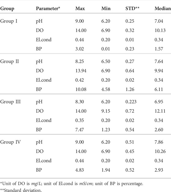
TABLE 3. Summary statistics of each group.

FIGURE 6

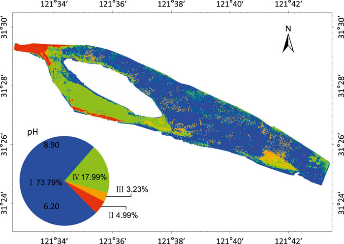
FIGURE 6. Clustering result of QCSR.

4 Discussion

4.1 Advantages of the novel framework

The design and application of the framework in our case study demonstrated its high performance in the monitoring and assessment of water quality. Compared to the previous studies, the advantages of this framework are summarized as follows.

CMT and RST are mutually integrated into the framework. CMT provides RST with sufficient in situ measurements, the prerequisite of the data set. In this study, the training data size provided by BioFish was nearly 500 times as many as the manual method within the same time interval Sagan et al. (2020); in addition, the geographic information of the data is not involved directly in the training and test process as input, which solves the problem of space-time limitation of the spatial interpolation methods to a certain extent. In the case of QCSR, the water quality parameters far from the cruise route, where no cruise route can be used nearby, can still be effectively inverted.

The environmental big data platform established by CMT and RST provides the basis for accurate environmental information interpretation. RST and CMT have the attributes of big data and good complementary so that the environmental big data platform can be built with the cooperation of the two parts. As shown in Figure 4, the results show an increasing trend of R² modelwise as the data size enlarges, indicating a significant advantage of environmental data analysis in contrast with the small or medium data platform.

On the big data platform, the adaptability and performance of deep learning ensure accuracy in monitoring and assessment. In Figure 4, break-even points can be observed at which the performance of DNN exceeds those of other traditional machine learning, especially when 40% or more data are fed. Through the encoder network with dimensions 4-125-125-500-10 and decoder network dimensions 10-500-125-125-4, original four-dimensional features (pH, DO, El.cond, and BP) are transferred into the new four-dimensional features, which contain much more information. Based on the updated four-dimensional features, clustering results are better than those based on the original four-dimensional features, meaning they are very close to the real world.

The novel framework formed a closed loop of water quality research, into which data collection, processing, monitoring, and assessment are packaged. In the framework, monitoring results can be mined for further assessment. Joint regional control strategies are more efficient and effective than single-point control strategies in environmental management and pollution control Zhang and Yang (2022). Deep clustering analysis enables the scientific delineation of joint control regions. Through the character analysis of the divided joint control area, characteristic factors of each area can be identified, which can contribute to defining a joint regional control strategy for the objective area. In this study, each group is managed as a joint control area, in a way that depends on the characteristic factors. Elevated BP (low water clarity) noted in the group II area may cause poor underwater light climate and loss of submerged macrophytes to switch the water body from a macrophyte-dominated state to an algae-dominated one Huang et al. (2021). In addition, the alkaline water body is one of the stimulatives for algae growth Lin et al. (2021). This means that the two water quality parameters, BP and pH, will be the focus of subsequent management and control of the distribution areas of group II and group IV, respectively.

To further ensure the reliability and accuracy of data collection, we have several particular strategies. 1) Seven calibrating points keep BioFish in a well-calibrated condition during the in situ measuring in order to assure the measuring accuracy. 2) The day of the satellite transit with cloud cover of less than 10 % was selected as the sampling day.

4.2 Potentiality of the developed framework

The developed framework as well as its three modularized parts show high potential in extensibility.

1) The environmental quality parameters were inverted by the developed framework by a data-driven approach instead of a physics- or chemistry-based one. Being data-driven makes results from the developed framework easily and rapidly transform into inversion of other environmental parameters collected by different sensors or CMT systems. The implementation was in the water scenario in this study. Alternately, this framework can be applicable to the air scenario when using an air quality CMT system.

2) The developed framework can realize the water quality monitoring in a timely manner by shortening the revisit time. The revisit time is defined as the time interval between two successive a satellite or a system’s observations on the same ground point on the surface of the Earth Luo et al. (2017). In this study, we chose the Sentinel-2 satellite system with a 5-day revisit time as the source of RST images. Accordingly, the need for 5-day monitoring of the whole target water bodies can be met with good weather conditions for RST observation and the availability of all parties (e.g., financing and labor). Selecting satellites with a shorter revisit time can increase the monitoring frequency, enabling the whole QCSR monitoring to keep pace with the environmental change of frequency, for example, replacing Sentinel-2 in this article with WorldView-3 (97 min revisit time) Ye et al. (2017).

A satellite with a spatial and spectral resolution provides a more precise inversion result and sharper clustering spatial boundaries by reducing the size of the raster within the objective area. As such, replacing Sentinel-2 in this article with WorldView-3 Ye et al. (2017) would obtain an up-to-date and more accurate result of inversion and clustering.

3) Our experiment in Section 3.1, 3.2 revealed that the performance of DNN is susceptible to the data size and gains a significant improvement as the data size increases. The reason can be seen in Figure 1B that each training iteration results in a model that is pretrained for the next training iteration after forward and backward calculations, and this process continues iteratively. Thus, we can expect a more robust and accurate model when more data are fed, such as more applications of the framework. More importantly, as the model was fed and trained by massive data, the in situ measuring might not be necessary.

4) The deep clustering method dealing with water quality assessment has advantages for big data sets with higher dimensional water quality parameters and multiple time periods. For processing high-dimensional water quality parameters, IDEC can have more objectives to extract and transform water quality features, which can make the clustering results closer to the real situation. In addition, deep clustering of the data for each time period separately allows for delineating newly integrated control areas and their characteristics. In this way, the overall state changes in the target water bodies can be seen at a glance, such as changes in the boundaries of each control area and changes in the characteristics of each control area.

4.3 Future work

Notwithstanding the developed work had several advantages, it is essential to note that improvements can be a part of future work.

RST images are significantly affected by weather conditions, especially cloud cover. An image with less than 35% cloud cover was regarded as a good practice to satisfy environmental monitoring requirements Marshall et al. (1994). To ensure accuracy, the “clear sky” images with less than 10% cloud cover were applied to the framework. Thus, there was a strict weather restriction during the in situ measuring. Sometimes the uncertainty of the weather can make in situ measurements fruitless, even though the plan is made according to the weather forecast.

Furthermore, the cruise monitor’s running does not synchronize with the satellite’s visit to the objective area. For instance, it takes Sentinel-2 less than 2 s to cross the QCSR. This lag prevents the satellite from being in real-time synchronization with the CMT measurements. In order to hurdle the weather limitations and eliminate the lag between RST and CMT measurements, we plan to introduce unmanned aerial vehicles (UAVs) associated with multispectral sensors into the framework. Its lower-than-cloud flight altitude reduces the interference of the cloud. In addition, the synchronized working pace of UAVs allows for simultaneous data collection along with the cruise monitor. As a supplementary element of the framework, UAVs are particularly applicable to small surface water areas like river bays and estuaries.

Last but not least, the performance of deep learning was essentially dependent on the data size. Hence, collecting more data from diverse types of water bodies should be a critical and indispensable work.

5 Conclusion

An innovative framework was developed with three modules: RST, CMT, and deep learning. Deep learning uses the big data platform created by RST and CMT to achieve a robust performance in water quality monitoring and assessment. Our testing revealed that the DNN (a type of deep learning) in the framework has a higher performance in monitoring four water quality parameters (pH, DO, El.cond, and BP) than MLR, SVR, and RFR. DNN is highly sensitive to training data size compared to other models, and the performance increases significantly with the elevated training data size. The application of IDEC on the water quality assessment showed that the entire QCSR was well-defined and divided into four groups as joint control areas, which are group I, group II, group III, and group IV. The characteristic factors of each area were identified, which can contribute to defining a joint regional control strategy for the QCSR. Considering the big data platform is the foundation of this framework, our future work in priority would be collecting more measured data (RST and CMT) from different water bodies to increase the capacity of the big data platform and update the deep learning model in our framework.

Data availability statement

The raw data supporting the conclusion of this article will be made available by the authors, without undue reservation.

Author contributions

Conceptualization: JQ; data curation: JQ and JB; formal analysis: JQ and LQ; funding acquisition: HL and SN; investigation: JQ, JB, and XX; methodology: JQ; project administration: SN and HL; resources: SN and HL; software: JQ and LQ; supervision: SN, HL, and YB; visualization: JQ; writing—original draft: JQ; writing—review and editing: SN, YB, QH, GY, QZ, and JB.

Funding

This work was supported by the National Natural Science Foundation of China (U2040210 and 31971477), and SIGN II—Amoris, BMBF (02WCL1471J).

Acknowledgments

The authors are grateful for the help from Andre Wilhelms for providing the basic information of BioFish and Xiaojie Zhang during in situ measuring. They also acknowledge support from the KIT-Publication Fund of the Karlsruhe Institute of Technology.

Conflict of interest

XX was employed by the company MioTech Research.

The remaining authors declare that the research was conducted in the absence of any commercial or financial relationships that could be construed as a potential conflict of interest.

Publisher’s note

All claims expressed in this article are solely those of the authors and do not necessarily represent those of their affiliated organizations, or those of the publisher, the editors, and the reviewers. Any product that may be evaluated in this article, or claim that may be made by its manufacturer, is not guaranteed or endorsed by the publisher.

Supplementary material

The Supplementary Material for this article can be found online at: https://www.frontiersin.org/articles/10.3389/fenvs.2022.979133/full#supplementary-material

References

Abdel-Rahman, E. M., Ahmed, F. B., and Ismail, R. (2013). Random forest regression and spectral band selection for estimating sugarcane leaf nitrogen concentration using EO-1 Hyperion hyperspectral data. Int. J. Remote Sens. 34, 712–728. doi:10.1080/01431161.2012.713142

CrossRef Full Text | Google Scholar

Agarap, A. F. (2018). Deep learning using rectified linear units (ReLU). arXiv e-printsarXiv:1803.08375.

Google Scholar

Berger, P. D., Maurer, R. E., and Celli, G. B. (2017). “Experimental design: With applications in management, engineering, and the sciences,” in Experimental design: With applications in management, engineering and the Sciences. Second edition. Cham, Switzerland: Springer Cham. chap. Multiple L. 505–507. doi:10.1007/978-3-319-64583-4

CrossRef Full Text | Google Scholar

Buma, W. G., and Lee, S. I. (2020). Evaluation of sentinel-2 and landsat 8 images for estimating chlorophyll-a concentrations in lake Chad, africa. Remote Sens. 12, 2437. doi:10.3390/RS12152437

CrossRef Full Text | Google Scholar

Chang, N. B., Imen, S., and Vannah, B. (2015). Remote sensing for monitoring surface water quality status and ecosystem state in relation to the nutrient cycle: A 40-year perspective. Crit. Rev. Environ. Sci. Technol. 45, 101–166. doi:10.1080/10643389.2013.829981

CrossRef Full Text | Google Scholar

Drusch, M., Del Bello, U., Carlier, S., Colin, O., Fernandez, V., Gascon, F., et al. (2012). Sentinel-2: ESA’s optical high-resolution mission for GMES operational services. Remote Sens. Environ. 120, 25–36. doi:10.1016/j.rse.2011.11.026

CrossRef Full Text | Google Scholar

Feyisa, G. L., Meilby, H., Fensholt, R., and Proud, S. R. (2014). Automated water extraction index: A new technique for surface water mapping using landsat imagery. Remote Sens. Environ. 140, 23–35. doi:10.1016/j.rse.2013.08.029

CrossRef Full Text | Google Scholar

Forkuor, G., Hounkpatin, O. K., Welp, G., and Thiel, M. (2017). High resolution mapping of soil properties using remote sensing variables in south-western Burkina Faso: A comparison of machine learning and multiple linear regression models. PLoS ONE 12, 01704788–e170521. doi:10.1371/journal.pone.0170478

CrossRef Full Text | Google Scholar

Guo, X., Gao, L., Liu, X., and Yin, J. (2017). Improved deep embedded clustering with local structure preservation. IJCAI Int. Jt. Conf. Artif. Intell. 0, 1753–1759. doi:10.24963/ijcai.2017/243

CrossRef Full Text | Google Scholar

Hassan, G., Goher, M. E., Shaheen, M. E., and Taie, S. A. (2021). Hybrid predictive model for water quality monitoring based on sentinel-2A L1C data. IEEE Access 9, 65730–65749. doi:10.1109/ACCESS.2021.3075849

CrossRef Full Text | Google Scholar

Holbach, A., Norra, S., Wang, L., Yijun, Y., Hu, W., Zheng, B., et al. (2014). Three Gorges Reservoir: Density pump amplification of pollutant transport into tributaries. Environ. Sci. Technol. 48, 7798–7806. doi:10.1021/es501132k

PubMed Abstract | CrossRef Full Text | Google Scholar

Huang, J., Qian, R., Gao, J., Bing, H., Huang, Q., Qi, L., et al. (2021). A novel framework to predict water turbidity using Bayesian modeling. Water Res. 202, 117406. doi:10.1016/j.watres.2021.117406

PubMed Abstract | CrossRef Full Text | Google Scholar

Ji, X., Dahlgren, R. A., and Zhang, M. (2016). Comparison of seven water quality assessment methods for the characterization and management of highly impaired river systems. Environ. Monit. Assess. 188, 15–16. doi:10.1007/s10661-015-5016-2

PubMed Abstract | CrossRef Full Text | Google Scholar

Kim, Y. H., Im, J., Ha, H. K., Choi, J. K., and Ha, S. (2014). Machine learning approaches to coastal water quality monitoring using GOCI satellite data. GIsci. Remote Sens. 51, 158–174. doi:10.1080/15481603.2014.900983

CrossRef Full Text | Google Scholar

Lee, S. J., Serre, M. L., van Donkelaar, A., Martin, R. V., Burnett, R. T., and Jerrett, M. (2012). Comparison of geostatistical interpolation and remote sensing techniques for estimating long-term exposure to ambient PM2.5 concentrations across the continental United States. Environ. Health Perspect. 120, 1727–1732. doi:10.1289/ehp.1205006

PubMed Abstract | CrossRef Full Text | Google Scholar

Li, J., and Heap, A. D. (2014). Spatial interpolation methods applied in the environmental sciences: A review. Environ. Model. Softw. 53, 173–189. doi:10.1016/j.envsoft.2013.12.008

CrossRef Full Text | Google Scholar

Lin, S. S., Shen, S. L., Zhou, A., and Lyu, H. M. (2021). Assessment and management of lake eutrophication: A case study in lake erhai, China. Sci. Total Environ. 751, 141618. doi:10.1016/j.scitotenv.2020.141618

PubMed Abstract | CrossRef Full Text | Google Scholar

Liu, H., Pan, D., and Chen, P. (2016a). A two-year field study and evaluation of water quality and trophic state of a large shallow drinking water reservoir in Shanghai, China. Desalination Water Treat. 57, 13829–13838. doi:10.1080/19443994.2015.1059370

CrossRef Full Text | Google Scholar

Liu, H., Pan, D., Zhu, M., and Zhang, D. (2016b). Occurrence and emergency response of 2-methylisoborneol and geosmin in a large shallow drinking water reservoir. Clean. Soil Air Water 44, 63–71. doi:10.1002/clen.201500077

CrossRef Full Text | Google Scholar

Luo, X., Wang, M., Dai, G., and Chen, X. (2017). A novel technique to compute the revisit time of satellites and its application in remote sensing satellite optimization design. Int. J. Aerosp. Eng., 1–9. doi:10.1155/2017/6469439

CrossRef Full Text | Google Scholar

Marçais, J., and de Dreuzy, J.-R. (2017). Prospective interest of deep learning for hydrological inference. Groundwater 55, 688–692. doi:10.1111/gwat.12557

CrossRef Full Text | Google Scholar

Marshall, G. J., Dowdeswell, J. A., and Rees, W. G. (1994). The spatial and temporal effect of cloud cover on the acquisition of high quality landsat imagery in the European Arctic sector. Remote Sens. Environ. 50, 149–160. doi:10.1016/0034-4257(94)90041-8

CrossRef Full Text | Google Scholar

Niu, C., Tan, K., Jia, X., and Wang, X. (2021). Deep learning based regression for optically inactive inland water quality parameter estimation using airborne hyperspectral imagery. Environ. Pollut. 286, 117534. doi:10.1016/j.envpol.2021.117534

PubMed Abstract | CrossRef Full Text | Google Scholar

Ortiz-Casas, J. L., and Peña-Martinez, R. (1989). Water quality monitoring in Spanish reservoirs by satellite remote sensing. Lake Reserv. Manag. 5, 23–29. doi:10.1080/07438148909354395

CrossRef Full Text | Google Scholar

Rolnick, D., and Tegmark, M. (2018). The power of deeper networks for expressing natural functions.” in 6th International Conference on Learning Representations, ICLR 2018 - Conference Track Proceedings, Vancouver, BC, Canada, April 30–May 3, 2018

Google Scholar

Sagan, V., Peterson, K. T., Maimaitijiang, M., Sidike, P., Sloan, J., Greeling, B. A., et al. (2020). Monitoring inland water quality using remote sensing: Potential and limitations of spectral indices, bio-optical simulations, machine learning, and cloud computing. Earth-Science Rev. 205, 103187. doi:10.1016/j.earscirev.2020.103187

CrossRef Full Text | Google Scholar

Shamai, G., and Kimmel, R. (2017). Geodesic distance descriptors.” in Proceedings - 30th IEEE Conference on Computer Vision and Pattern Recognition CVPR, Honolulu, HI, USA, July 21–26, 2017, 3624. doi:10.1109/CVPR.2017.386

CrossRef Full Text | Google Scholar

Simeonov, V., Stratis, J. A., Samara, C., Zachariadis, G., Voutsa, D., Anthemidis, A., et al. (2003). Assessment of the surface water quality in Northern Greece. Water Res. 37, 4119–4124. doi:10.1016/S0043-1354(03)00398-1

PubMed Abstract | CrossRef Full Text | Google Scholar

Singh, K. P., Malik, A., and Sinha, S. (2005). Water quality assessment and apportionment of pollution sources of Gomti river (India) using multivariate statistical techniques - a case study. Anal. Chim. Acta 538, 355–374. doi:10.1016/j.aca.2005.02.006

CrossRef Full Text | Google Scholar

Stork, C. L., and Autrey, B. C. (2005). Remotely mapping river water quality using multivariate regression with prediction validation. Remote Sens. Model. Ecosyst. Sustain. II 5884, 588408. doi:10.1117/12.616852

CrossRef Full Text | Google Scholar

Udy, J., Gall, M., Longstaff, B., Moore, K., Roelfsema, C., Spooner, D. R., et al. (2005). Water quality monitoring: A combined approach to investigate gradients of change in the great barrier reef, Australia. Mar. Pollut. Bull. 51, 224–238. doi:10.1016/j.marpolbul.2004.10.048

PubMed Abstract | CrossRef Full Text | Google Scholar

Vo-Van, T., Nguyen-Hai, A., Tat-Hong, M. V., Nguyen-Trang, T., and Gomariz, F. (2020). A new clustering algorithm and its application in assessing the quality of underground water. Scientific Programming. doi:10.1155/2020/6458576

CrossRef Full Text | Google Scholar

Wagle, N., Acharya, T. D., and Lee, D. H. (2020). Comprehensive review on application of machine learning algorithms for water quality parameter estimation using remote sensing data. Sensors Mater. 32, 3879–3892. doi:10.18494/SAM.2020.2953

CrossRef Full Text | Google Scholar

Ye, B., Tian, S., Ge, J., and Sun, Y. (2017). Assessment of WorldView-3 data for lithological mapping. Remote Sens. 9, 1132–1219. doi:10.3390/rs9111132

CrossRef Full Text | Google Scholar

Yuan, Q., Shen, H., Li, T., Li, Z., Li, S., Jiang, Y., et al. (2020). Deep learning in environmental remote sensing: Achievements and challenges. Remote Sens. Environ. 241, 111716. doi:10.1016/j.rse.2020.111716

CrossRef Full Text | Google Scholar

Zhan, H., Lee, Z., Shi, P., Chen, C., and Carder, K. L. (2003). Retrieval of water optical properties for optically deep waters using genetic algorithms. IEEE Trans. Geosci. Remote Sens. 41, 1123–1128. doi:10.1109/TGRS.2003.813554

CrossRef Full Text | Google Scholar

Zhang, D. D., Xie, F., and Zhang, L. (2019). Preprocessing and fusion analysis of GF-2 satellite Remote-sensed spatial data.” in Proceedings of 2018 International Conference on Information Systems and Computer Aided Education, Changchun, China, July 6–8, 2018. ICISCAE, 24. doi:10.1109/ICISCAE.2018.8666873

CrossRef Full Text | Google Scholar

Zhang, L., and Yang, G. (2022). Cluster analysis of PM2.5 pollution in China using the frequent itemset clustering approach. Environ. Res. 204, 112009. doi:10.1016/j.envres.2021.112009

PubMed Abstract | CrossRef Full Text | Google Scholar

Zhao, Q., and Fränti, P. (2014). WB-Index: A sum-of-squares based index for cluster validity. Data Knowl. Eng. 92, 77–89. doi:10.1016/j.datak.2014.07.008

CrossRef Full Text | Google Scholar

Zhong, S., Zhang, K., Bagheri, M., Burken, J. G., Gu, A., Li, B., et al. (2021). Machine learning: New ideas and tools in environmental science and engineering. Environ. Sci. Technol. 55, 12741–12754. doi:10.1021/acs.est.1c01339

PubMed Abstract | CrossRef Full Text | Google Scholar