 Haixu Yu
 He Wang1
- 1School of Business, Southern University of Science and Technology, Shenzhen, China
- 2School of Economics and Management, Harbin Institute of Technology, Shenzhen, China
In recent years, carbon market transactions have become more active. The number of countries participating in carbon market regulation is increasing, and the carbon market’s overall turnover continues to grow. It is important to study the features of carbon allowance price volatility for the stable development of the carbon market. This paper constructs a modified ICSS-GARCH model to analyze the volatility of carbon price returns and the dynamic characteristics of price fluctuations in the emissions trading system of the European Union (EU-ETS) and the Chinese carbon pilot markets in Hubei. The results show that fluctuations in carbon price returns have a leverage effect and that the impact of negative news on the market is stronger than that of positive news. The international climate and energy conferences, abnormal changes in traditional energy prices, and global public health emergencies all affect volatility and cause shocks to the carbon trading market. The modified ICSS-GARCH model with structural breaks can reduce the pseudovolatility of the return series to a certain extent and can improve the accuracy of the model. This research can give policymakers some implications about how to develop the carbon market and help market participants control the risks of fluctuations in carbon allowances. Regulators should enhance carbon price monitoring and focus on short-term shocks in the carbon market to reduce trading risks. The Chinese carbon market should strengthen the system design and develop carbon financial derivatives.
1 Introduction
Countries around the world are taking steps to reduce emissions of greenhouse gases such as carbon dioxide because of climate change and other environmental and ecological problems (Can et al., 2022). To reduce carbon emissions, many countries have signed the United Nations Framework Convention on Climate Change (UNFCCC), the Kyoto Protocol and the Paris Agreement, etc. The Kyoto Protocol outlines the obligations of developed economies to reduce emissions and proposes three flexible mechanisms to reduce emissions, of which carbon trading is one (Can et al., 2021b). According to the International Carbon Action Partnership’s (ICAP) Emissions Trading Worldwide Status Report 2021, there are currently 25 emissions trading system (ETS) in operation around the world, with another 22 scheduled to go operational in the near future. Carbon emissions trading will cover 17% of global emissions. The existing trading systems include EU emissions trading system (EU-ETS) and US trading system (RGGI), etc.
The EU-ETS was established in 2005 and is currently the world’s largest and most active carbon emissions trading system. EU-ETS carbon allowances trading reaches 8,1 billion tons of carbon dioxide (CO2) in 2020, representing approximately 90 percent of the total global carbon trading volume, with a trading volume of €20 billion. It has been implemented in four phases and is currently in its fourth phase. In the first three phases of EU-ETS development, the range of countries, industries and enterprises covered by trading gradually expanded, and the proportion of auctions in the allowance allocation process gradually increased (instead of free allocation). The major difference between the three phases is the change from grandparenting1 to benchmarking2 in the allocation of allowances, indicating the continuous maturation of the EU-ETS management system. In the EU-ETS, the turnover of EUAs is higher than that of other trading varieties, such as certified emission reductions (CERs). EU allowance (EUA) futures allow carbon credits to be traded on commodity futures exchanges, such as soybeans, oil, and other commodities. The EU-ETS has become the world’s largest carbon futures market, with over 90% of the total volume traded in the EU carbon market (Lamphiere et al., 2021). The carbon futures market has made the market more open and has become a model for other countries and regions.
According to the International Energy Agency (IEA), China’s carbon emissions exceed 11.9 billion tons in 2021, covering about one-third of the world’s carbon emissions. The Chinese government announced at the Paris Climate Conference that CO2 emissions will peak around 2030 and then decline by 60–65 percent compared to 2005. China is exploring the use of market mechanisms to reduce greenhouse gas emissions in response to the pressures of CO2 emission reduction and sustainable development. As an important developing country and CO2 emitter, China expects that the carbon market will help achieve its emissions reduction objectives and reduce the global greenhouse effect at the lowest economic cost among the available emission reduction policies (Liu et al., 2015; Gozgor and Can, 2017). Since 2013, China has initiated eight regional carbon market pilots in Shenzhen, Shanghai, Beijing, Guangdong, Tianjin, Hubei, Chongqing, and Fujian (Ren and Lo, 2017). The pilot markets have been operational for only a short period, and there are still some unstable factors in the carbon market (Zhao et al., 2016). The carbon market in China covered about 3,000 emitting enterprises in the steel, electricity, and cement industries, establishing a large-scale market initially. China’s carbon emissions trading market has grown to become the world’s second largest, and it now plays an important role in the international energy trading market. Under these circumstances, it is more important and urgent to study how carbon prices change in both the EU-ETS market and the Chinese carbon market.
Both the EU carbon market and the Chinese carbon pilot cover significant emission sectors such as industry and power. However, because of the different development processes, there are many differences between the two markets. The major variation is in the allocation of carbon allowances. The auction is employed in the EU-ETS, with the European Commission determining the overall number of carbon allowances and allocating them to each member. The auction method ensures the scarcity of carbon allowances. The Chinese carbon market adopts the free allocation approach and is susceptible to surplus. Both the EU-ETS and Chinese markets have excess carbon allowances, leading to a carbon price failure. The Chinese market is particularly affected. Chinese carbon credits can only be traded on the spot market. The diversity of carbon financial instruments and trading activity is restricted compared to the EU-ETS.
In recent years, the effectiveness of carbon markets, the volatility and risk assessment of carbon prices, and the spillover effects between carbon markets and traditional energy markets have been hot topics (Benz and Truck, 2009; Chevallier, 2009; Zhang and Sun, 2016; Chang et al., 2017; Zhao et al., 2020; Can et al., 2021a). In prior studies, time series of financial asset markets, such as the stock market or crude oil market, and structural breaks have been widely studied as the iterative cumulative sum of squares (ICSS) algorithm for detecting breaks is now well established (Malik and Hassan, 2004; Malik et al., 2005; Wen et al., 2018). However, less research has been conducted on structural breaks in carbon markets. Price volatility in the carbon market is influenced by external factors such as political change, climate change, and allowance allocation. External factors cause carbon price instability and risk spillover. Moreover, exploring the reasons and mechanisms of structural breaks is important for carbon market policymakers to effectively adjust market policies. In this paper, we adopt the modified ICSS algorithm to investigate the structural breaks in carbon market returns and add structural breaks as a dummy variable in the model to estimate the volatility characteristics of the EU-ETS and the Chinese carbon market.
The current research on carbon market volatility is mainly focused on the EU-ETS. In the existing literature, the volatility of carbon prices, the factors influencing carbon prices, the effectiveness of carbon markets, and the measurement of risk in carbon markets have been examined. Benz and Truck (2009) and Daskalakis et al. (2009) analyzed the European carbon market and found that emission allowance returns exhibit skewness, excess kurtosis, and volatility clustering. Byun and Cho (2013) used the GARCH model to estimate the price volatility of carbon futures prices. Dutta (2018) used the GARCH-jump model to investigate the volatility of the EU-ETS prices and provide recommendations to investors and policymakers. Guo et al. (2018) used the GARCH model to analyze the impact of the EU-ETS emission announcements in phases I and II on trading behavior and prices. The findings confirm the maturity of the EU-ETS in phase II. Fan et al. (2017) analyzed the impact of 50 policy announcements from the EU ETS on carbon prices. The aggregate impacts of the 50 events studied were small, and only sections of the policies impacted carbon prices. Wang et al. (2019) demonstrated that all externalities of the carbon market, whether energy prices or policy announcements, are reflected in trading behavior and they impact the demand and supply of carbon permits through trading, which influences carbon pricing (Wang et al., 2019). Zhang et al. (2018) adopted the EGARCH model to examine the price of carbon pilot markets in China and discovered a long memory in the sequence of carbon price returns. Zhao et al. (2016) demonstrated that the market efficiency of ETS pilots in China is not satisfactory, although ETS system designs have achieved some promising preliminary results.
In this paper, we compare the price of EUA futures, the most actively traded variant in the EU-ETS, with the spot price of the Chinese carbon pilot market and analyze the price fluctuations in the carbon market. This paper makes the following contributions to the existing literature: Firstly, to the best of our knowledge, prior studies have concentrated on the value-at-risk of the carbon market while disregarding the impact of structural breaks on risk assessments, thus making carbon market risk underestimated (Zhang et al., 2018). Our research is a useful supplement. Secondly, we noticed that policy announcements and important events can cause structural changes in carbon price returns, which can have an impact on the carbon market or create market risks. We detect the structural change points by using the modified ICSS algorithm. We then use the structural change points as dummy variables to study how event shocks affect the volatility of the carbon market. This is a novel approach in the study of carbon market volatility to incorporate structural breaks estimated by the modified ICSS algorithm into carbon market volatility research. Furthermore, we explore the asymmetry of the carbon price. This is an extension of the study of the characteristics of carbon market prices. The findings confirm that carbon price returns are also asymmetrical and that the impact of positive and negative news on the carbon price varies, which is similar to those of other financial assets. These important results and conclusions will be used to make important suggestions about how the carbon finance market will grow in the future and how governments and market participants will manage such a market and invest in it.
The remainder of this paper is structured as follows. Section 2 is a literature review. Section 3 introduces the methodologies used in this paper. Section 4 reports the empirical results. Section 5 provides further discussion on EU-ETS futures in phase II and provides policy recommendations. Section 6 provides the conclusions of the paper.
2 Related literature
2.1 Carbon price volatility
In previous papers, time series of financial asset markets, such as the stock market or crude oil market, with structural breaks have been widely studied with the iterative cumulative sum of squares (ICSS) algorithm for detecting breaks now well established (Malik and Hassan, 2004; Malik et al., 2005; Wen et al., 2018). However, less research has been done on structural breaks in carbon markets.
The carbon market is an emerging financial market. Existing literature on carbon markets is mainly focused on carbon prices, including carbon market volatility, factors influencing carbon prices, carbon market effectiveness, and carbon market risk measurement.
For example, Benz and Truck (2009) and Daskalakis et al. (2009) analyzed the European carbon market and found that emission allowance returns exhibit skewness, excess kurtosis, and volatility clustering. Byun and Cho (2013) estimated the volatility of carbon futures prices using IV, k-NN, and GARCH-type models. The results indicate that the GJR-GARCH model offers the most information on the volatility of carbon futures. Paolella and Taschini (2008) found asymmetries in the spot carbon price, which are essential for risk management in the carbon market. Dutta (2018) tested for extreme values in EUA and investigated the volatility of EU-ETS prices using the GARCH-jump model. The results demonstrate that the GARCH-jump model can capture discrete jumps in asset returns. Outliers and time-varying jumps play a crucial role in the risk management of the carbon market. Wang et al. (2019) demonstrated that all externalities of the carbon market, whether energy prices or policy announcements, are reflected in trading behavior and impact the demand and supply of carbon permits via trading, which influences carbon pricing. Gorenflo (2013) investigates the price efficiency of EUA futures and spot. The results show that futures markets are better at finding prices than spot markets, with carbon futures playing a bigger role.
Numerous studies have examined the performance of the carbon market in China. For example, Zhang et al. (2018) adopted the EGARCH model to examine the price of carbon pilot markets in China and discovered a long memory in the sequence of carbon price returns. Lyu et al. (2020) investigates the dynamic characteristics of volatility using the MCMC-SV model and Chinese carbon price returns in Hubei, Shenzhen, and Shanghai from 2015 to 2018. The results demonstrate that the Chinese carbon prices indicate an aggregation of volatility, although the long-term volatility is not highly cyclical. Zhao et al. (2016) demonstrated that the market efficiency of ETS pilots in China is not satisfactory, with huge price differences and insufficient liquidity across ETS pilots, although ETS system designs have achieved some promising preliminary results. This result was caused by the inappropriate allocation of allowances and the low motivation of businesses to trade. Liu et al. (2020) examined the operational efficiency of China’s seven carbon markets, using a variance ratio test. The findings suggest that the markets in Hubei and Guangdong are weakly efficient, while the remainder of the markets are less efficient.
Prior research indicates that the modified ICSS model has been widely utilized in measuring the volatility of financial assets and is capable of analyzing the volatility of carbon market prices (Malik and Hassan, 2004; Wen et al., 2018). In addition, a comparative study of EU-ETS and Chinese carbon pilot markets could help the carbon market develop better.
2.2 EU-ETS and China carbon pilots
The EU Emissions Trading System (EU-ETS), established in 2005, is a carbon trading mechanism based on EU regulations and national legislation. The EU-ETS is the world’s most developed carbon trading system and dominates the international carbon financial market. Currently, the EU-ETS is in its fourth phase, following three phases of development and gradual improvement. During previous phases of development, the carbon market’s coverage of covered sectors and gases gradually expanded, and the proportion of auctions in the allowance allocation process gradually increased. Table 1 shows the difference between the different phases of EU-ETS.
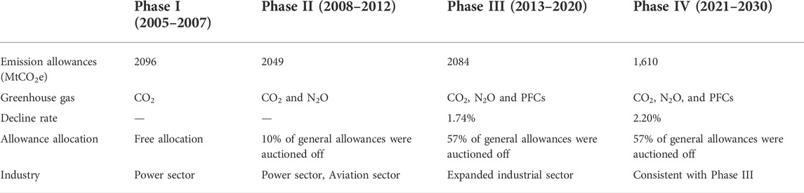
TABLE 1. Characteristics of the different phases of EU-ETS.
In the EU-ETS, the turnover of EUAs is higher than that of other trading varieties, such as certified emission reductions (CERs). In this paper, EUA futures phase III prices are used to analyze the behavior of price volatility in the carbon market, while phase II prices are used for the comparative analysis. Figure 1 shows the price trend of EUA futures from 2005 to 2021.
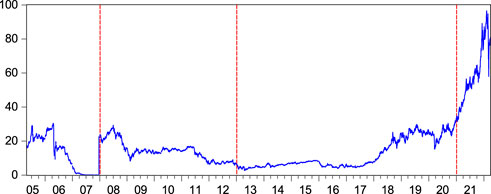
FIGURE 1. Price trends in EUA futures. The vertical lines mark the beginning of the different phases: phase I (2005–2007), phase II (2008–2012), phase III (2013–2020), and phase IV (2020–present).
The carbon market was immature during the first phase of the EU-ETS due to a lack of experience with relevant allocations. In the first phase, numerous factors affected the futures price, and there were significant price fluctuations. Because of the inability to store Phase I and Phase II allowances across phases, the EUA price fell to an all-time low of €0.01 at the end of 2007, undermining the effectiveness of the EU-ETS market. In the second and third phases, the European Commission revised the trading mechanism and the way allowances are allocated. Since 2008, EUA futures prices have shown regular changes, influenced by global economic trends and energy prices. The EU-ETS matured after the initial two stages of exploration and development. Thus, this paper analyzes the volatility characteristics of futures prices in the third stage.
As the main supplier of demand for clean development mechanism (CDM) projects, China participates in worldwide emission reduction missions. In 2013, China established eight regional ETS pilots. The pilots have different prices, turnover, and volumes. Figure 2 shows the price trend for the major pilots. The price trend of each carbon pilot in China is different, and the eight carbon market pilots have their own transaction rules and systems. Furthermore, most studies use trading data from the carbon pilots in Shenzhen, Guangdong, and Hubei because these three pilots have higher market shares and liquidity than other carbon pilots (Fan and Todorova, 2017; Chang et al., 2018; Zhao et al., 2020). The Hubei spot price is used in this study because it is the largest market in terms of turnover and is relatively active and mature.
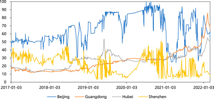
FIGURE 2. Price trends of major carbon pilots in China, including the Beijing, Guangdong, Hubei, and Shenzhen pilots.
3 Methodology
3.1 Modified ICSS algorithm
The iterative cumulative sums of squares (ICSS) algorithm was proposed by Inclan and Tiao (1994). This method is used to distinguish structural break points of volatility based on the cumulative sum (CUSUM) test statistic. At the start of the process, the method assumes that the variance of the time series is the same for a certain period of time. The variance changes at the time of the unexpected event and then remains constant. There is a sudden structural change during an event. The procedure is as follows.
Assume that the sample has T observations and that the residual sequence of the sample
where
The ICSS algorithm assumes that
Previous research has shown that event shocks can cause structural break points in time series (Malik, 2003). Dummy variables incorporated into the model can reduce the pseudovolatility of the return series and improve model accuracy. The modified ICSS algorithm is used to detect structural break points in the following study. We use the news to determine which major events they correspond to and add them to the model as dummy variables.
3.2 GARCH model
Engle (1982) proposed the autoregressive conditional heteroskedasticity (ARCH) model for studying the volatility of asset prices. Bollerslev (1986) proposed the generalized ARCH (GARCH) model. The GARCH model adds the lagged values of the conditional variance across periods to the ARCH model to describe the long memory of financial assets. The GARCH (p, q) model is given by the following equation:
where
3.3 Exponential GARCH model
Many studies have found a leverage effect in financial assets. The leverage effect is caused by the fact that negative returns have a greater impact on future volatility than positive returns (Christie, 1982). The exponential GARCH (EGARCH) model was proposed by Nelson (1991). On the left side of the model equation, the conditional variance is logarithmized. This model overcomes the critical limitation of GARCH models, which is parameter nonnegativity. The conditional variance equation of the EGARCH (1, 1) model is given by the following equation.
The
If the coefficient of the asymmetric term
The normal distribution, which forms the basis of portfolio theory, may not necessarily apply to financial asset price patterns. Therefore, we assume that the residuals follow a generalized error distribution (GED) in the following analysis. The distribution is given by the following equation.
where v is the degrees of freedom.
3.4 Modified ICSS-GARCH model
In this paper, we adopt the AR (1)-GARCH (1, 1) model to fit the EUA futures returns and MA (1)-GARCH (1, 1) to fit the Hubei spot returns. The ICSS-GARCH models used to describe the EUA futures returns and Hubei spot returns are shown in Eqs 9, 10, respectively.
4 Empirical analysis
4.1 Data
In this paper, we collect a dataset of EUA futures prices and Hubei carbon spot prices. In this part, we use data on EUA futures from phase III. The sample period for EUA futures is from 1 January 2013, to 31 December 2020. The sample period for spot prices on the Hubei carbon market is from 1 July 2019, to 30 July 2021, encompassing two emissions trading compliance periods. The Chinese carbon market is still in the development stage. To better capture price fluctuations, we chose data from recent years. The logarithm of the prices is used to calculate all yield series data.
where
Figure 3 shows the trend of returns. It can be noted that the sample is stationary, but simultaneously shows volatility clustering. Furthermore, all of the return series in the figure are subject to extreme volatility.
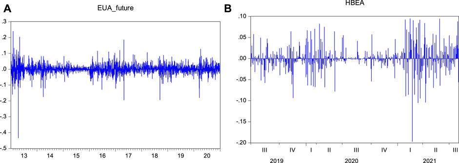
FIGURE 3. Carbon price yield trends. (A) EUA futures return trend; (B) Hubei spot price return trend. The sample period is from 1 January 2013, to 31 December 2020, for EUA futures and from 1 July 2019, to 30 July 2021, for Hubei spot returns.
4.2 Descriptive analysis
Table 2 shows the basic characteristics of EUA futures and Hubei spot returns. The minimum values of the two returns are −0.4347 and −0.1972. The maximum values of the EUA futures returns and Hubei spot returns are 0.2405 and 0.0952, respectively. Meanwhile, the mean value of the EUA futures returns is 0.0008 and the mean value of Hubei spot returns is 0.0001. The standard deviations of EUA futures returns and Hubei spot returns are 0.0342 and 0.0306, respectively. The kurtosis of all the return series exceeds three, and the skewness of these returns is not equal to zero. The skewness of the EUA futures return is greater than zero, indicating a right-skewed distribution. The skewness of the Hubei spot return is less than zero, indicating a left-skewed distribution. The two series have the same characteristics as other financial time series, with higher peaks and fatter tails.
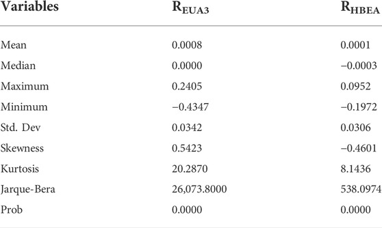
TABLE 2. Data descriptive statistics. This table presents the descriptive statistics results of carbon price returns considered for the whole sample period. JB denotes the Jarque-Bera test statistic for the null of normality.
The JB statistic shows that none of the return series follow a normal distribution. Figure 4 indicates that the quantile-quantile plot test results confirm this as well. Therefore, using the generalized error distribution (GED) to characterize the data in the modeling approach in this paper can more accurately explain the statistical features of the carbon return series.
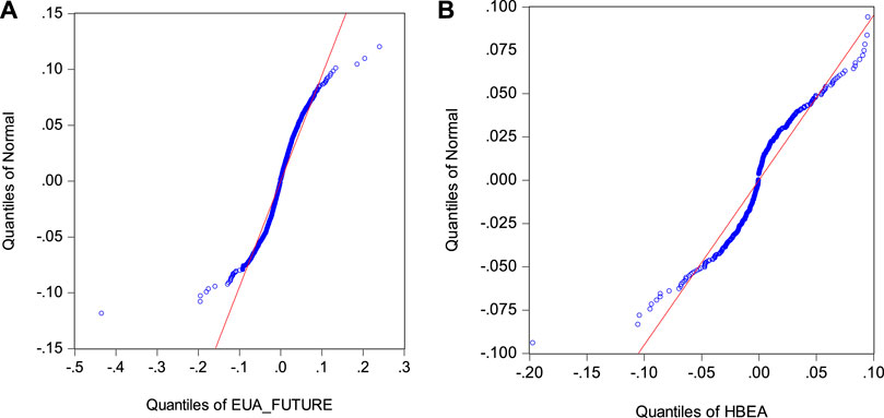
FIGURE 4. Quantile-quantile plots for returns. (A) EUA futures; (B) Hubei spot. The sample period is from January 1, 2013, to December 31, 2020, for EUA futures and from July 1, 2019, to July 30, 2021, for Hubei spot returns.
4.3 Carbon price volatility characteristics
In this part, we examine the volatility characteristics of the series because the GARCH family model requires the series to be stable and to have conditional heteroskedasticity. Thus, before we establish the GARCH models, it is essential to test whether the two series are stationary and heteroskedastic.
4.3.1 Unit-root test
We examine whether the series is stationary by using the Augmented Dickey Fuller (ADF) test. Table 3 shows the results from the ADF test. The results for the EUA futures and Hubei spot return series all reject the null hypothesis, since the t-statistic values are equal to 0.0000, indicating that the two series are both stationary.

TABLE 3. ADF test of EUA futures and Hubei spot returns. The null hypothesis of the ADF test is the presence of a unit root, that is, the series is nonstationary.
4.3.2 ARCH-LM test
We examine whether the series is heteroskedastic by using the ARCH-LM test. We regress the return series on the constant term to obtain the residual series and take the lags of order 1, order 5, and order 10 for the test. Table 4 shows the results of the ARCH effect test for the return series. Both the F-statistic and LM-statistic are significantly larger than the critical values, and the residuals of the return series have conditional heteroskedasticity. This means that the GARCH family of models can be used.
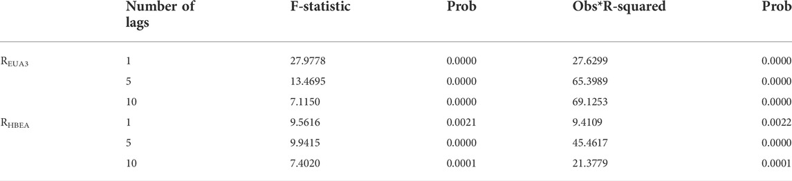
TABLE 4. ARCH-LM test results. The null hypothesis is that a series of residuals exhibits no conditional heteroscedasticity. The p-value represents the significance of the corresponding test.
4.4 Empirical results
In this part, we perform a modeling analysis of carbon price returns. First, we use the EGARCH model to evaluate the impact of positive and negative news on returns. Then, we use the modified ICSS algorithm to locate structural breaks in the returns and find the times when structural changes occur; then, we introduce them into the GARCH model as dummy variables to investigate the impact of event shocks on return volatility. In this paper, some of the structural breaks are generated at the time corresponding to the associated announcement in the news and are added to the model as dummy variables to investigate the impact of event shocks on return volatility. In further discussions, we compare data from phases II and III of EUA futures to see if there is continuity in the causes driving structural fractures.
4.4.1 Leverage effect analysis based on the EGARCH model
It is known that the volatility of financial assets tends to be asymmetric, which means that good news and bad news have different impacts on financial assets (Nelson, 1991). Therefore, this paper establishes an EGARCH model to study the leverage effect of the volatility of carbon return series. Table 5 shows the estimation results for the EUA futures. The fluctuations of EUA futures and Hubei spot returns are asymmetric, i.e., rises and falls in carbon price returns have different effects on future volatility. In addition, the coefficient of the asymmetric term γ is −0.0340, indicating that there is a leverage effect on the impact of carbon return volatility and that the impact of negative news on carbon market volatility is greater than that of positive news. Positive news generates a shock of a factor of 0.2023 (
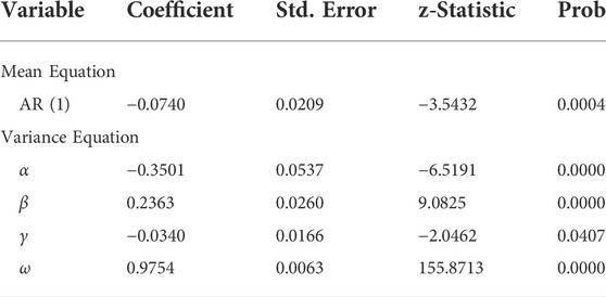
TABLE 5. Estimation results of the EGARCH (1, 1) model for EUA futures returns from 1 January 2013, to 31 December 2020.
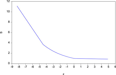
FIGURE 5. News impact curve of the EGARCH (1, 1) model of EUA futures returns.
Table 6 shows the estimation results for the Hubei spot returns. Although the coefficient γ of the asymmetric term of the Hubei spot returns is less than 0, the asymmetric term is not statistically significant, which means that there is no significant leverage effect. The reason is that China’s carbon trading market is still at an early stage of development, and the main trading entities are enterprises whose emissions are controlled. In addition, China only has a spot trading market, which is less active than the EU market. After years of development and innovation, the EU-ETS has become more mature, with a broader investor structure and larger trade volume. Thus, compared to its traditional financial market, China’s carbon market still needs to be developed.
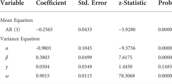
TABLE 6. Estimation results of the EGARCH (1, 1) model for Hubei spot returns from 1 July 2019, to 30 July 2021.
4.4.2 Volatility analysis based on the modified ICSS-GARCH model
4.4.2.1 Structural break tests based on the modified ICSS algorithm
Using the modified ICSS algorithms presented in Section 2, we begin by detecting the structural breaks. We set the significance level for the algorithms at 0.05. Table 7 shows the results of structural break tests for the carbon market using the modified ICSS algorithm. There are nine structural change points in the EUA futures returns and four structural change points in the Hubei spot returns in the sample period. In this paper, some of the structural breaks are generated at the time corresponding to their announcement in the news and are added to the model as dummy variables. We find that the international climate and energy conferences, abnormal changes in prices of traditional energy such as oil, and global public health emergencies all affect the volatility of the carbon market and cause certain shocks to the carbon trading market.
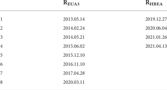
TABLE 7. Structural breaks of EUA futures and Hubei spot returns.
Table 8 shows the events that occurred on the dates corresponding to the structural breaks; the results indicate that the major event shocks caused the variance to change structurally. Next, we add the structural breaks as dummy variables to the GARCH model to compare how important events affect the volatility of carbon prices.
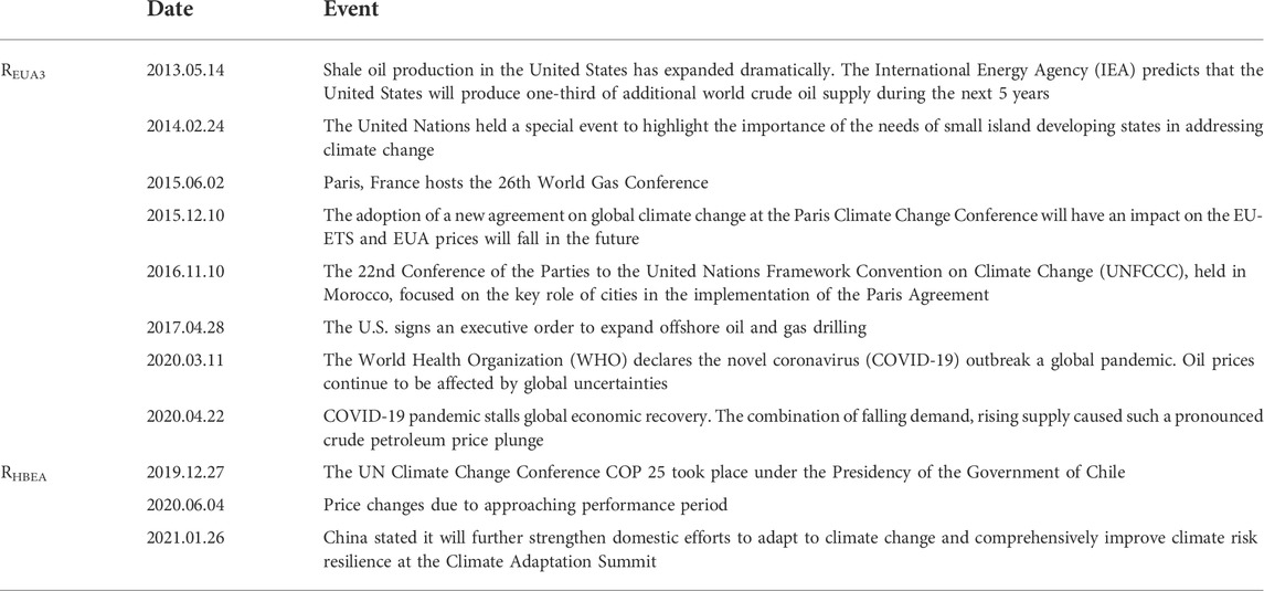
TABLE 8. Events corresponding to structural breaks.
4.4.2.2 Analysis of the GARCH model based on structural breaks
Using the modified ICSS algorithm, we have found structural breaks. Then we introduce them into the GARCH model for comparative analysis. We compare two models: one without structural change points and the other with structural change points, which are given individually in both cases.
4.4.2.2.1 GARCH model without structural breaks
First, we use the GARCH model without structural breaks. Tables 9, 10 show the estimation results of the GARCH model. For EUA futures and Hubei spot returns, all parameters are significant. The coefficients of α and β in the model are positive, and their sum is close to 1, indicating that the volatility of the carbon market has persistence and long memory.
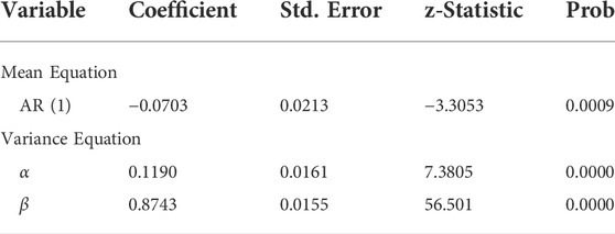
TABLE 9. Parameter estimates of the AR (1)–GARCH (1, 1) model for EUA futures returns in phase III, without structural breaks from 1 January 2013, to 31 December 2020.
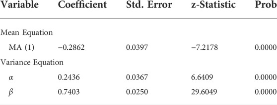
TABLE 10. Parameter estimates of the MA (1)—GARCH (1, 1) model for Hubei spot returns without structural breaks from 1 July 2019, to 30 July 2021.
4.4.2.2.2 GARCH model with structural breaks
We adopt the modified ICSS-GARCH model to further analyze the volatility characteristics of the carbon market. Tables 11, 12 illustrate the results of the estimation. We find that the characteristics of volatility are attenuated when we consider structural breaks. We observe a decrease in the sum of α and β for both EUA futures and Hubei spot returns. The sum of α and β for EUA futures returns decreases from 0.9933 to 0.9870, and the sum of α and β for Hubei spot returns decreases from 0.9838 to 0.9730. This indicates that the strong persistence and long memory characteristics of volatility become weaker after we add the structural breaks as a dummy variable to the model. The modified ICSS-GARCH model reduces the pseudovolatility of the return series and enhances the model’s accuracy (Malik et al., 2005).
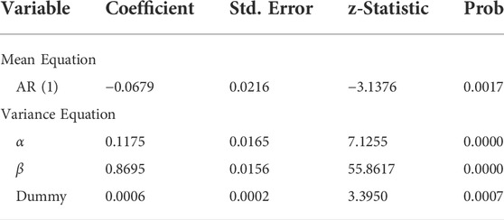
TABLE 11. Parameter estimates of the AR (1)—GARCH (1, 1) model for EUA futures returns in phase III, with structural breaks from 1 January 2013, to 31 December 2020.

TABLE 12. Parameter estimates for the MA (1)—GARCH (1, 1) model for Hubei spot returns with structural breaks from 1 July 2019, to 30 July 2021.
Table 13 depicts the results of the ARCH-LM test for the residuals after we model the return series. The p-value of the residual series is greater than 0.05 for lag orders of 1, 5 and 10, and therefore the null hypothesis is accepted. This shows that after modeling, the conditional heteroskedasticity in the series is removed, which means that the model fits well.

TABLE 13. ARCH-LM test results for residual series. The null hypothesis is that a series of residuals exhibits no conditional heteroscedasticity. The p-value represents the significance of the corresponding test.
5 Further discussion
5.1 Analysis of EU-ETS phase II
We replace our dataset with the EU-ETS phase II trading data for further discussion of the volatility of EUA futures’ returns. Due to data availability, the scope for the prices of EUA futures’ returns is from 2 January 2008, to 31 December 2012. Table 14 illustrates the basic characteristics of EUA futures returns in phase II. The descriptive statistics show that the mean value of the return in phase II is -0.0010, which is lower than the value of 0.0008 in phase III, indicating that the return of EUA futures is gradually increasing. The standard deviation of phase II is 0.0271, which is not significantly different from phase III, and the price fluctuation is more stable. In addition, the returns of both phases have the characteristics of higher peaks and fatter tails and do not follow a normal distribution.

TABLE 14. Phase II data descriptive statistics. This table presents the descriptive statistics results of carbon price returns considered for the whole sample period. JB denotes the Jarque-Bera test statistic for the null of normality.
We also conducted ADF and ARCH-LM tests on the data of EUA futures in phase II, and the results show that the returns remain stationary and the residuals of the return series are conditionally heteroskedastic. Next, we analyze the volatility of EUA futures returns in phase II using the same methods as in Section 3.
The estimation results for the EGARCH (1, 1) model are shown in Table 15. The fluctuations in phase II of the EUA futures are asymmetric. The coefficient of the asymmetric term γ is −0.0674, indicating that there is a leverage effect on the impact of carbon return volatility and that the impact of negative news on carbon market volatility is greater than that of positive news. Positive news generates a shock of a factor of 0.1475 (
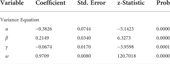
TABLE 15. Estimation results of the EGARCH (1, 1) model of EUA futures returns in phase II from 2 January 2008, to 31 December 2012.
We examine the structural break points uncovered by using the modified ICSS algorithms. There are four structural breaks in the EUA futures returns in phase II: they occurred on 21 October 2008; 16 June 2009; 28 May 2010; and 22 June 2011. We also add these structural breaks to the model as dummy variables. Table 16 illustrates the estimation results of the GARCH (1, 1) model without the structural breaks. Table 17 shows the results of the ICSS-GARCH (1, 1) model with structural breaks. The findings show that the characteristics of volatility are attenuated once we consider structural breaks. There is a decrease in the sum of α and β for both phases. The sum of α and β for EUA futures returns decreases from 0.9936 to 0.9847.
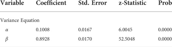
TABLE 16. Parameter estimates of the GARCH (1, 1) model for EUA futures returns in phase II without structural breaks from 2 January 2008, to 31 December 2012.
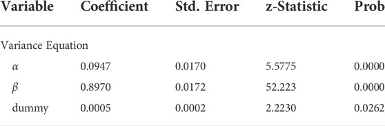
TABLE 17. Parameter estimates of the GARCH (1, 1) model for EUA futures returns in phase II with structural breaks from 2 January 2008, to 31 December 2012.
This is consistent with the findings for phase III, in which EU-ETS volatility does not change significantly between the two phases, confirming that phase II volatility characteristics persist into phase III. This also indicates that the strong persistence and long memory characteristics of volatility become weaker after we add the structural breaks as dummy variables to the model. The modified ICSS-GARCH model reduces the pseudovolatility of the return series and enhances the model’s accuracy. A proper assessment of short-term price and volatility is a critical issue in the carbon market since effectively measuring volatility risk is critical for carbon market managers in a complex market.
To summarize, our study shows the following findings: First, there is a leverage effect on the impact of carbon return volatility, and the impact of negative news on carbon market volatility is greater than that of positive news. This is consistent with previous research demonstrating that the returns on financial assets are leveraged and that positive and negative news have different impacts on return volatility (Paolella and Taschini, 2008; Dutta, 2018). Secondly, we find that the international climate and energy conferences, abnormal changes in prices of traditional energy such as oil, and global public health emergencies all affect the volatility of the carbon market and cause certain shocks to the carbon trading market. Wang et al. (2019) demonstrated that all externalities of the carbon market, whether energy prices or policy announcements, are reflected in trading behavior and impact the demand and supply of carbon permits via trading, which influences carbon pricing. We extend this conclusion. Finally, our results are consistent with previous results using the modified ICSS-GARCH model to study financial market data (Malik et al., 2005; Wen et al., 2020). The results show that the modified ICSS-GARCH model is also applicable to the study of carbon market volatility and that the model can reduce the pseudovolatility of the return series to a certain extent and improve the accuracy of the model.
5.2 Policy recommendations
The findings of this study are potentially significant for further research into carbon emission permits. They help policymakers and investors in the carbon market identify risks and develop strategies to minimize them.
Firstly, regulators should enhance carbon price monitoring and focus on short-term shocks in the carbon market to reduce trading risks. Studies have shown that when the carbon market is subject to exogenous shocks, prices are prone to dramatic fluctuations and the market does not compensate for potential risks. Market managers should recognize and identify abnormal price fluctuations and forecast the trend. In addition, market management should establish stability reserves in order to minimize extreme price changes in response to exogenous shocks, reduce trade risks, and improve market stability.
Second, the Chinese carbon market should improve the system design. The findings indicate that the EU-ETS price is less volatile and more stable than the carbon market in China. In the short term, the Chinese carbon market is inactive, participants are risk-averse, and products lack diversity. In the long term, the Chinese carbon market needs a comprehensive development plan and a well-structured market framework. It still needs to be improved in many ways, and the design of the system should be strengthened.
Finally, the Chinese market should boost the development of carbon finance instruments. Chinese carbon credits can only be traded on the spot market. To increase the liquidity of the carbon market, policymakers should encourage the development of derivative products such as carbon futures, which can diversify investment portfolios and attract more investors to participate in trading. Stability in the carbon market can be established through the use of derivatives for price discovery and risk aversion. Prior studies suggest that the EU-ETS reduces the volatility of spot prices after the introduction of futures products, and spreads the uncertainty of spot prices through a hedging mechanism (Chevallier et al., 2011). Furthermore, derivatives can be used for price discovery and risk aversion in order to stabilize the carbon market. It can also increase market activity and encourage both institutional and individual investors to trade actively in the carbon market.
6 Conclusion
Responding to climate change, realizing carbon emission reductions at the lowest cost by economic market means and reversing the increasing trend of greenhouse gas emissions are major challenges for the world.
In this paper, we investigate the volatility characteristics of the EU-ETS and the Chinese Hubei carbon market, by using the modified ICSS-GARCH model. The study shows the following findings. 1) There is a leverage effect on the impact of carbon return volatility, and the impact of negative news on carbon market volatility is greater than that of positive news. The leverage effect in the Hubei carbon market was not statistically significant during the sample period. We surmise that this result could be due to inactive market trading and trading entity limits. 2) We find that the international climate and energy conferences, abnormal changes in prices of traditional energy such as oil, and global public health emergencies all affect the volatility of the carbon market and cause certain shocks to the carbon trading market. 3) We adopt the modified ICSS algorithm to find the structural breaks and introduce them as dummy variables to investigate the impact of event shocks on the volatility of the carbon market. The results indicate that the ICSS-GARCH model can reduces the pseudovolatility of the return series to a certain extent and improve the accuracy of the model. In addition, our results hold after we replace the data from EUA futures phase III with those from phase II, indicating that our model is robust and that the factors affecting phase II persist into phase III.
Our findings could be important for carbon emission permit research. They help policymakers and investors identify risks and develop prevention measures. Regulators can minimize trade risks by enhancing monitoring of carbon prices. Policymakers should improve the way the system is set up and speed up the development of carbon finance instruments for the Chinese carbon market.
Data availability statement
The CSV data used to support the findings of this research are available from the corresponding author upon request.
Author contributions
HY: conceptualization, software, data curation, and writing original draft; HW: methodology, reviewing, and editing; CL: software, data curation, and writing original draft; ZL: methodology, reviewing, and editing; SW: conceptualization, supervision, and funding acquisition.
Funding
This research is supported and funded by the 13th Five-Year Plan of Philosophy and Social Sciences in Guangdong Province-Discipline Co-Construction (No. GD18XYJ36) and Shenzhen Humanities and Social Sciences Key Research Bases.
Acknowledgments
The authors are grateful to editor and two anonymous referees for insightful comments and suggestions.
Conflict of interest
The authors declare that the research was conducted in the absence of any commercial or financial relationships that could be construed as a potential conflict of interest.
Publisher’s note
All claims expressed in this article are solely those of the authors and do not necessarily represent those of their affiliated organizations, or those of the publisher, the editors and the reviewers. Any product that may be evaluated in this article, or claim that may be made by its manufacturer, is not guaranteed or endorsed by the publisher.
Footnotes
1Grandparenting allows covered enterprises to get emission permits based on their previous emissions within a base year or base period.
2Benchmarking rewards efficient installations and can more easily assimilate new entrants.
References
Benz, E., and Truck, S. (2009). Modeling the Price Dynamics of CO2 Emission Allowances. Energy Econ. 31 (1), 4–15. doi:10.1016/j.eneco.2008.07.003
Bollerslev, T. (1986). Generalized Autoregressive Conditional Heteroskedasticity. J. Econom. 31 (3), 307–327. doi:10.1016/0304-4076(86)90063-1
Byun, S. J., and Cho, H. (2013). Forecasting Carbon Futures Volatility Using GARCH Models with Energy Volatilities. Energy Econ. 40, 207–221. doi:10.1016/j.eneco.2013.06.017
Can, M., Ahmad, M., and Khan, Z. (2021a). The Impact of Export Composition on Environment and Energy Demand: Evidence from Newly Industrialized Countries. Environ. Sci. Pollut. Res. 28 (25), 33599–33612. doi:10.1007/s11356-021-13084-5
Can, M., Ahmed, Z., Mercan, M., and Kalugina, O. A. (2021b). The Role of Trading Environment-Friendly Goods in Environmental Sustainability: Does Green Openness Matter for OECD Countries? J. Environ. Manage. 295, 113038. doi:10.1016/j.jenvman.2021.113038
Can, M., Ben Jebli, M., and Brusselaers, J. (2022). Can Green Trade Save the Environment? Introducing the Green (Trade) Openness Index. Environ. Sci. Pollut. Res. 29 (29), 44091–44102. doi:10.1007/s11356-022-18920-w
Chang, K., Chen, R. D., and Chevallier, J. (2018). Market Fragmentation, Liquidity Measures and Improvement Perspectives from China's Emissions Trading Scheme Pilots. Energy Econ. 75, 249–260. doi:10.1016/j.eneco.2018.07.010
Chang, K., Pei, P., Zhang, C., and Wu, X. (2017). Exploring the Price Dynamics of CO2 Emissions Allowances in China's Emissions Trading Scheme Pilots. Energy Econ. 67, 213–223. doi:10.1016/j.eneco.2017.07.006
Chevallier, J. (2009). Carbon Futures and Macroeconomic Risk Factors: A View from the EU ETS. Energy Econ. 31 (4), 614–625. doi:10.1016/j.eneco.2009.02.008
Chevallier, J., Le Pen, Y., and Sévi, B. (2011). Options Introduction and Volatility in the EU ETS. Resour. Energy Econ. 33 (4), 855–880. doi:10.1016/j.reseneeco.2011.07.002
Christie, A. A. (1982). The Stochastic Behavior of Common Stock Variances: Value, Leverage and Interest Rate Effects. J. Financ. Econ. 10 (4), 407–432. doi:10.1016/0304-405X(82)90018-6
Daskalakis, G., Psychoyios, D., and Markellos, R. N. (2009). Modeling CO2 Emission Allowance Prices and Derivatives: Evidence from the European Trading Scheme. J. Bank. Finance 33 (7), 1230–1241. doi:10.1016/j.jbankfin.2009.01.001
Dutta, A. (2018). Modeling and Forecasting the Volatility of Carbon Emission Market: The Role of Outliers, Time-Varying Jumps and Oil Price Risk. J. Clean. Prod. 172, 2773–2781. doi:10.1016/j.jclepro.2017.11.135
Engle, R. F. (1982). Autoregressive Conditional Heteroscedasticity with Estimates of the Variance of United Kingdom Inflation. Econometrica 50 (4), 987–1007. doi:10.2307/1912773
Engle, R. F., and Ng, V. K. (1993). Measuring and Testing the Impact of News on Volatility. J. Finance 48 (5), 1749–1778. doi:10.1111/j.1540-6261.1993.tb05127.x
Fan, J. H., and Todorova, N. (2017). Dynamics of China's Carbon Prices in the Pilot Trading Phase. Appl. Energy 208, 1452–1467. doi:10.1016/j.apenergy.2017.09.007
Fan, Y., Jia, J. J., Wang, X., and Xu, J. H. (2017). What Policy Adjustments in the EU ETS Truly Affected the Carbon Prices? Energy Policy 103, 145–164. doi:10.1016/j.enpol.2017.01.008
Gorenflo, M. (2013). Futures Price Dynamics of CO2 Emission Allowances. Empir. Econ. 45 (3), 1025–1047. doi:10.1007/s00181-012-0645-6
Gozgor, G., and Can, M. (2017). Does Export Product Quality Matter for CO2 Emissions? Evidence from China. Environ. Sci. Pollut. Res. 24 (3), 2866–2875. doi:10.1007/s11356-016-8070-6
Guo, J. F., Su, B., Yang, G., Feng, L. Y., Liu, Y. P., and Gu, F. (2018). How Do Verified Emissions Announcements Affect the Comoves between Trading Behaviors and Carbon Prices? Evidence from EU ETS. Sustainability 10 (9), 3255. doi:10.3390/su10093255
Inclan, C., and Tiao, G. C. (1994). Use of Cumulative Sums of Squares for Retrospective Detection of Changes of Variance. J. Am. Stat. Assoc. 89 (427), 913–923. doi:10.2307/2290916
Lamphiere, M., Blackledge, J., and Kearney, D. (2021). Carbon Futures Trading and Short-Term Price Prediction: An Analysis Using the Fractal Market Hypothesis and Evolutionary Computing. Mathematics 9 (9), 1005. doi:10.3390/math9091005
Liu, L. W., Chen, C. X., Zhao, Y. F., and Zhao, E. D. (2015). China's Carbon-Emissions Trading: Overview, Challenges and Future. Renew. Sustain. Energy Rev. 49, 254–266. doi:10.1016/j.rser.2015.04.076
Liu, X., Zhou, X., Zhu, B., and Wang, P. (2020). Measuring the Efficiency of China’s Carbon Market: A Comparison between Efficient and Fractal Market Hypotheses. J. Clean. Prod. 271, 122885. doi:10.1016/j.jclepro.2020.122885
Lyu, J., Cao, M., Wu, K., Li, H., and Mohi-ud-din, G. (2020). Price Volatility in the Carbon Market in China. J. Clean. Prod. 255, 120171. doi:10.1016/j.jclepro.2020.120171
Malik, F., Ewing, B. T., and Payne, J. E. (2005). Measuring Volatility Persistence in the Presence of Sudden Changes in the Variance of Canadian Stock Returns. Can. J. Economics-Revue Can. D Econ. 38 (3), 1037–1056. doi:10.1111/j.0008-4085.2005.00315.x
Malik, F., and Hassan, S. A. (2004). Modeling Volatility in Sector Index Returns with GARCH Models Using an Iterated Algorithm. J. Econ. Finan. 28 (2), 211–225. doi:10.1007/bf02761612
Malik, F. (2003). Sudden Changes in Variance and Volatility Persistence in Foreign Exchange Markets. J. Multinatl. Financial Manag. 13 (3), 217–230. doi:10.1016/S1042-444X(02)00052-X
Nelson, D. B. (1991). Conditional Heteroskedasticity in Asset Returns: A New Approach. Econometrica 59 (2), 347–370. doi:10.2307/2938260
Paolella, M. S., and Taschini, L. (2008). An Econometric Analysis of Emission Allowance Prices. J. Bank. Finance 32 (10), 2022–2032. doi:10.1016/j.jbankfin.2007.09.024
Ren, C., and Lo, A. Y. (2017). Emission Trading and Carbon Market Performance in Shenzhen, China. Appl. Energy 193, 414–425. doi:10.1016/j.apenergy.2017.02.037
Sansó, A., Aragó, V., and Carrion, J. L. (2004). Testing for Changes in the Unconditional Variance of Financial Time Series. Rev. Econ. Financ. 4, 32–52.
Wang, J. Q., Gu, F., Liu, Y. P., Fan, Y., and Guo, J. F. (2019). Bidirectional Interactions between Trading Behaviors and Carbon Prices in European Union Emission Trading Scheme. J. Clean. Prod. 224, 435–443. doi:10.1016/j.jclepro.2019.03.264
Wen, F. H., Zhao, L. L., He, S. Y., and Yang, G. Z. (2020). Asymmetric Relationship between Carbon Emission Trading Market and Stock Market: Evidences from China. Energy Econ. 91, 104850. doi:10.1016/j.eneco.2020.104850
Wen, F., Xiao, J., Huang, C., and Xia, X. (2018). Interaction between Oil and US Dollar Exchange Rate: Nonlinear Causality, Time-Varying Influence and Structural Breaks in Volatility. Appl. Econ. 50 (3), 319–334. doi:10.1080/00036846.2017.1321838
Zhang, Y.-J., and Sun, Y.-F. (2016). The Dynamic Volatility Spillover between European Carbon Trading Market and Fossil Energy Market. J. Clean. Prod. 112, 2654–2663. doi:10.1016/j.jclepro.2015.09.118
Zhang, Y. P., Liu, Z. X., and Xu, Y. Y. (2018). Carbon Price Volatility: The Case of China. Plos One 13 (10), e0205317. doi:10.1371/journal.pone.0205317
Zhao, L. L., Wen, F. H., and Wang, X. (2020). Interaction Among China Carbon Emission Trading Markets: Nonlinear Granger Causality and Time-Varying Effect. Energy Econ. 91, 104901. doi:10.1016/j.eneco.2020.104901
Keywords: carbon market volatility, EU-ETS, ICSS algorithm, GARCH model, Chinese carbon market
Citation: Yu H, Wang H, Liang C, Liu Z and Wang S (2022) Carbon market volatility analysis based on structural breaks: Evidence from EU-ETS and China. Front. Environ. Sci. 10:973855. doi: 10.3389/fenvs.2022.973855
Received: 20 June 2022; Accepted: 08 August 2022;
Published: 26 September 2022.
Edited by:
Muhlis Can, BETA Akademi-SSR Lab, TurkeyReviewed by:
Nurhan Toguc, Istanbul Esenyurt Üniversity, TurkeyIhsan Oluç, Mehmet Akif Ersoy University, Turkey
Copyright © 2022 Yu, Wang, Liang, Liu and Wang. This is an open-access article distributed under the terms of the Creative Commons Attribution License (CC BY). The use, distribution or reproduction in other forums is permitted, provided the original author(s) and the copyright owner(s) are credited and that the original publication in this journal is cited, in accordance with accepted academic practice. No use, distribution or reproduction is permitted which does not comply with these terms.
*Correspondence: Susheng Wang, d2FuZ3NzQHN1c3RlY2guZWR1LmNu