Drivers of spatiotemporal disparities in the supply-demand budget of ecosystem services: A case study in the Beijing-Tianjin-Hebei urban agglomeration, China

Assessing the spatiotemporal patterns of ecosystem services (ESs) supply and demand, as well as the drivers thereof during specific time periods, is critical for regional policy making and sustainable management. Taking the Beijing-Tianjin-Hebei (BTH) urban agglomeration of China as an example, we studied four ES supply-demand budgets: carbon storage, water provision, food provision and soil conservation from 2000 to 2015. Through the geodetector model, canonical analysis and Multiscale Geographically Weighted Regression (MGWR) model, the drivers of the ES supply-demand budget were explored. The results showed that the areas supplying high amounts of ESs in the northern region usually did not overlap those areas consuming intensive ESs, which were mainly distributed in metropolitan areas. The anthropological factors, including per capita gross domestic product (Per.GDP) and population density (POP.Den), were the dominant influencing factors for the imbalance between the supply and demand of carbon storage, water provision and food provision, which were mainly distributed in the central and southern regions of the study area. Geomorphological factors (ELE and SLO) were the key driving factors of soil conservation, which was mainly distributed in the eastern regions. In all, our findings could provide comprehensive information for decision-making and ES management.

Introduction

Ecosystem services (ESs) are defined as the various benefits that people obtain from ecosystems, which helps maintain global life support systems (Costanza et al., 1997; Daily et al., 2009; Raoet al., 2018). They are necessary for human well-being as they provide multiple functions including food, water, timber, minerals, climate regulation, water purification, soil erosion prevention, and recreation (Nelson et al., 2009; Cruz-Garcia et al., 2017). Over the past three decades, global changes such as climate change, population increase, rapid urbanization, technological development and policy making have threatened and affected large-scale natural ecosystem structures and functions as never before, causing severe modifications in ESs and threatening human well-being (Mooney et al., 2009; Nelson et al., 2009). In response to this background, a growing number of scientists have been working on mapping and analyzing ES supply (Minin et al., 2017; Wilkerson et al., 2018). Landscapes are geospatially heterogeneous, socioeconomically driven, regionally coupled systems of human-environment interaction (Sun et al., 2019). Most of these prior studies have focused mainly on exploring ES supply changes under the effects of climate, land-use changes and topographical factors (Peng et al., 2017; Borrelli et al., 2020; Li et al., 2021).

Nevertheless, the status of ESs is not only influenced by the supply capacity of ecosystems, but also driven by human demands and desires for different kinds of ESs (Wei et al., 2017; Yu et al., 2021). On the one hand, ES supply is generally defined as the ecological products and services provided by eco-systems to human society based on biophysical characteristics, ecological functions and social characteristics (de Groot et al., 2010). ES demand, on the other hand, can be described as the actual use or consumption of ESs by stakeholders in a particular area within a given time, which is affected by socioeconomic system and has received increased attention in the last 10 years (Burkhard et al., 2012; Schirpke et al., 2019). However, because of the complex coupling between social systems and natural ecosystems, focusing on only one side of ESs will lead to an imbalance between ES supply and demand, causing unexpected ecological concerns and social equity issues (Baró et al., 2016; Delphin et al., 2016). Therefore, incorporating ES demand side into ES assessments can help decision makers identify ES supply and demand surplus and deficit and provide a scientific basis for achieving regional sustainable development goals (Costanza et al., 2017; Schirpke et al., 2019).

Previous studies have assessed spatial dynamic variations in ES supply and demand (Burkhard et al., 2012; Chen et al., 2019; Xu et al., 2021); clarified the spatial matching of ES supply and demand, such as the ratio of supply to demand (Boithias et al., 2014; Bryan et al., 2018); and evaluated the mismatch between ES supply and demand to inform regional management (Larondelle and Lauf, 2016). These studies help us understand the mismatch between ES supply and demand in different contexts (Ahmad et al., 2020; Yao et al., 2021). However, improving the matching of ES supply and demand is still a significant challenge in the crusade to meet human needs and demands (Mehring et al., 2018). To attain a balance, it is necessary to comprehensively manage land use and other social resources to avoid ES deficit–defined as the ES supply cannot meet ES demand (the value of ES gap is lower than 0) (Cui et al., 2019). Although it has been proven that land use, climate, topographical and socio-economic factors significantly influence ES supply and demand, few studies have comprehensively explored the drivers of ES supply and demand as a whole (Costanza et al., 2017; Chaplin-Kramer et al., 2019). Furthermore, current studies lack discussions on the scale dependence in the spatially non-stationary relationships between driving factors and ES supply and demand.

The Beijing-Tianjin-Hebei (BTH) urban agglomeration is densely populated, and is one of the regions with the most rapid economic and urbanization development in the world. It suffers from serious environmental problems, such as air pollution, water and soil loss, water scarcity and biodiversity loss (Li et al., 2017; Yang et al., 2019), which leads to the losses of regional ESs (Zhang et al., 2017). Therefore, this study chose the BTH urban agglomeration as a case to evaluate the supply, demand, and gap of ESs and their drivers the spatial scale, which can enrich researches in this field. This study has three specific objectives: 1) to quantify the spatial and temporal variations of four critical ES supply and demand from 2000 to 2015, including carbon storage (CS), water provision (WP), food provision (FP), and soil conservation (SC); 2) to examine the spatiotemporal patterns of the mismatches between ES supply and demand at the county or district scale; and 3) to explore the key drivers of the mismatches between ES supply and demand and analyze the spatial heterogeneity of these effects. This study aims to propose several land-use strategies and socioeconomic and ecological management measures that can alleviate ES mismatches, supporting regional ecological security and sustainable development.

Materials and methods

This study proposed a framework to assess the effects of anthropological, climate factors, and geomorphological factors on ESDRs and support regional ES management in the Beijing-Tianjin-Hebei urban agglomeration (Figure 1). Firstly, relevant data were collected and three comprehensive factors was measured. Secondly, the spatio-temporal variations of comprehensive factors and four ES supply-demand ratio (ESDRs) were evaluated from 2000 to 2015. Thirdly, relationships between ESDRs and anthropological, climate factors, and geomorphological factors was analyzed by using geodetector model, RDA, and GWR model. Finally, some relevant policy recommendations and measures were put forward.

FIGURE 1

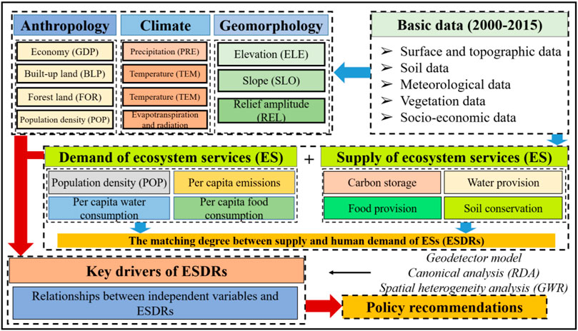
FIGURE 1. The framework and procedures of this study.

Study area

The BTH urban agglomeration, located in Northern China (35°03′–42°40′N, 113°27′–119°50′E, Figure 2), borders the Taihang Mountain, Yanshan Mountain and Bohai Bay. It covers an area of 212,962 km², including two municipalities (Beijing and Tianjin city), as well as Hebei province with 11 prefectural-level cities, amounting to 173 counties. The northwestern part of this region has a higher elevation and is mostly hilly, while the southeast is relatively flat with an elevation of less than 100 m. The BTH urban agglomeration has a temperate continental climate, with an annual mean precipitation of 420–550 mm and an annual mean temperature of −3.5° to 24.5°C (Shen, J et al., 2020). The southeastern plain is an important grain production area in China, growing corn, wheat, and peanuts.

FIGURE 2

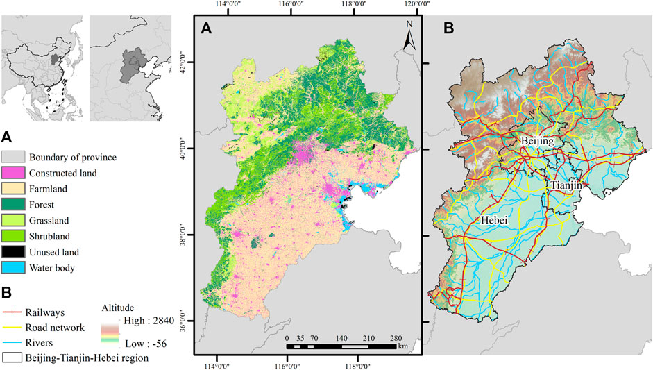
FIGURE 2. Study area. (A) LULC distribution of cover-types. (B) Map of major rivers and urban and peri-urban infrastructure, including roads, railway, and municipal boundaries.

The BTH urban agglomeration is a political, cultural, and economic center in China. In 2019, BTH created a GDP of 8.46 trillion yuan, accounting for 8.5% of the country’s GDP. From 2000 to 2019, the urbanization of this region developed rapidly. The urbanization rate increased from 38.50% in 2000 to 66.70% in 2019. The urban population of the BTH urban agglomeration increased from 70.91 million to 113.07 million. With its high-density population and high rate of urbanization, the region has experienced long-term water resource shortages and unbalanced development between the sown area and grain yield (Li et al., 2017). Moreover, the imbalance between resource supply and demand has triggered a series of regional problems, including surface runoff decrease, land desertification, groundwater over-extraction, air quality deterioration, biodiversity reduction, and eco-system degradation (Zhang et al., 2017; Yang et al., 2019). Therefore, a comprehensive diagnosis of ESs from the sup-ply-demand perspective is highly significant for BTH’s sustainable ES management.

Data sources

Five types of data were used in this study: land-use, statistical, meteorological, geomorphological, and soil (Supplementary Table S1). Land use data were obtained from the Resource and Environ-mental Science Data Center of the Chinese Academy of Sciences (http://www.resdc.cn/). We adopted the classification system proposed in the “Current Land Use Classification” formulated by the Ministry of Natural Resources of China (Ministry of Natural and Re-sources of R.P.C) as the basic classification system (Ministry of Natural and Resources of R.P.C, 2017). Land use was classified into seven types: grassland, water body, cultivated land, artificial surface, unused land, forest land, and shrub land. All vector and raster data were converted to the same projection coordinate system (Bei-jing_1954_3_Degree_GK_CM_ 114E), and the spatial accuracy of all raster data was modified to 30 m by resampling in ArcGIS 10.3.

Quantification of ecosystem services supply and demand

In this work, four key ESs were selected according to the latest version of the Common International Classification of ES (CICES). The selected ESs are very important for the sustainable development of the BTH urban agglomeration and are sensitive to global climate changes, land use changes and significantly increased human activities (CICES, https://cices.eu/resources/). Table 1 provides an overview of the ESs evaluated in the study area and the reasons for their selections by literature reviews.

TABLE 1

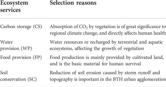
TABLE 1. Ecosystem services evaluated in the Beijing-Tianjin-Hebei urban agglomeration.

Carbon storage

(1) Supply

Carbon storage (CS) refers to the capacity of vegetation to store carbon, which is essential for climate change mitigation (Onaindia et al., 2013). Here, the “InVEST carbon storage model” was used to quantify carbon storage based on land use maps and four carbon pools: 1) above-ground biomass (CS_a); 2) below-ground biomass (CS_b); 3) soil organic matter (CS_s); and 4) dead organic matter (CS_d) (Sharp et al., 2020). The carbon stocks per unit area for each land use type were derived from literature based on local studies (Tallis and Polasky, 2009). The total carbon stored SCS for each pixel (Mg) was calculated as:

$SCS=PA\left({CS}_A+{CS}_b+{CS}_c+{CS}_d\right)(1)$

where PA is the pixel area (30 × 30 m = 900 m² or 0.09 ha), CS_a is the above-ground carbon density (Mg C·ha⁻¹); CS_b is the below-ground carbon density (Mg C·ha⁻¹); CS_s is the soil organic carbon density (Mg C·ha⁻¹); and CS_d is the dead organic matter carbon density (Mg C·ha⁻¹).

(2) Demand

The total amount of carbon emissions was used as the demand for carbon storage in this study, as the changes of per capita emissions will lead to an increase or decrease of the demand for carbon sequestration (Bateman et al., 2013). The total amount of carbon emission is calculated by multiplying the total energy consumption by the standard carbon emission coefficient according to the data provided by CO₂ emission inventory of BTH (e.g. residential, industry, and agriculture) (BMBS, 2015; HMBS, 2015; TMBS, 2015). The amount of carbon contained in CO₂ was estimated to be about 27% of total carbon. We multipled the average value of emissions per capita by the population density to obtain the total carbon emitted per pixel (González-García et al., 2020). The calculation of total amount of carbon emissions is as follow:

$D_{CP}=D_{pcfc}\times D_{pop}(2)$

where DCP is the demand for carbon sequestration (t), Dpcfc is the per capita carbon emissions (t); and Ppop is the population density (person·km²). For details, please refer to Supplementary Table S2.

Water provision

(1) Supply

Water provision (WP) refers to the annual quantity of water yield available to humans within a given region (Boithias et al., 2014). The “Hydropower Water Yield module” of InVEST was used to quantify water provision based on the Budyko curve, with the data including average annual precipitation, root restricting layer depth (mm), plant available water content, annual reference evapotranspiration (mm), and land use maps (Sharp et al., 2020). The calculation of annual water provision Y for each pixel is as follows:

$Y=\left(\mathit{1}-AET/P\right).P(3)$

$AET/P=\left(\mathit{1}+PET/P\right)-{\left[\mathit{1}+{\left(PET/P\right)}^{\omega }\right]}^{\mathit{1}/\omega }(4)$

$PET=K.E{T}_{\mathit{0}}/P(5)$

$\omega =Z.AWC/P+1.25(6)$

$AWC=\mathit{Min}\left(Rest.layer.SoilDepth,Root.Depth\right).PAWC(7)$

where AET is the annual actual evapotranspiration (mm); P is the annual precipitation (mm); AET/P is based on an expression of the Budyko curve proposed by (Fu, 1981; Zhang et al., 2004); PET is the potential evapotranspiration, ω is an empirical parameter that characterizes the natural climatic-soil properties; ET0 is the reference evapotranspiration; K is the vegetation evapotranspiration coefficient associated with the land use (Sharp et al., 2020); AWC is the volumetric plant available water content; Z is the empirical constant, and sometimes referred to as “seasonality factor” (1–30); and PAWC is the Plant Available Water Content fraction (0–1) (Sharp et al., 2020).

(2) Demand

Water demand (D_WY) refers to the total amount of water consumption for agricultural and industrial production, inhabitants, and ecological purposes (Burkhard et al., 2013; Chen et al., 2019). For this estimate, we collected the population density map and the water resource bulletins from each county which provides the water consumption per inhabitant per studied year (BMBS, 2015; HMBS, 2015; TMBS, 2015). The calculations of water demand D_WY is as follows:

$D_{WY}=D_{pcwc}\times P_{pop}(8)$

where D_pcwc is the per capita water consumption; and P_pop is the population density (person·km²). For details, please refer to Supplementary Table S3.

Food provision

Both the supply and demand for food provision (FP) were estimated through statistical data. Here, for FP supply, we first added up each county’s production of grain, vegetables, and fruit products, which were the three main types of foods produced in cropland (https://data.cnki.net/Yearbook/Navi?type=type&code=A). Then, we estimated the demand for FP by multiplying the per capita food consumption by the population density. According to (Tang and Li, 2012), the per capita food demand was 322.07 kg·a-1, which can basically meet China’s per capita food security. For counties without per capita food consumption data, city or provincial-scale per capita food consumption was used as an alternative. Food provision supply and demand can be calculated using the following equations:

$S_i^{FP}={{\displaystyle \sum }}_j^n{P}_{\left(i,j\right)}\left(j=\mathit{1,2,3}\dots ,n\right)(9)$

$D_i^{FP}=D_{pcfp}\times P_{pop}(10)$

where $S_i^{FP}$is the FP supply for county I; P (i, j) is the annual provision of j type food for each county, including grains, vegetables and fruits; $D_i^{FP}$ is the FP demand for county I; $D_{pcfp}$ is the per capita food demand; and $P_{pop}$ is the population density (person·km²).

Soil conservation

(1) Supply

The “Sediment Delivery Ratio module” of InVEST was used to map and calculate the total amount of soil conservation per pixel based on the universal soil loss equation (RUSLE) (Sharp et al., 2020). Soil conservation equals the difference between the actual amount of soil erosion (USLE) and the maximum potential amount of soil erosion (RKLS), assuming the original land cover without the C or P factors (Kareiva et al., 2011; Ouyang et al., 2016), and is calculated as:

$SC=RKLS-usle(11)$

$usle=R.K.LS.C.P(12)$

$RKLS=R.K.LS(13)$

where SC is the amount of soil conservation (tons · ha−1 · yr−1); usle is the amount of actual soil loss (tons · ha−1 · yr−1); RKLS is the amount of potential soil loss (tons · ha−1 · yr−1); R is rainfall erosivity (MJ · mm (ℎa · ℎr)−1); K is the soil erodibility factor for each pixel (MJ · mm (ℎa · ℎr)−1); LS is the slope length-gradient factor (dimensionless); and C and P are the crop management and support practice factors for each pixel (dimensionless), respectively.

(2) Demand

The amount of actual soil loss was used to define demand for soil conservation, which is based on the quantity of actual soil erosion that human beings are expected to deal with (Liu et al., 2019). The calculation of the amount of actual soil loss is below:

$usle=R.K.LS.C.P(14)$

where usle is the amount of actual soil loss (tons · ha−1 · yr−1). For details, please refer to Supplementary Table S4.

Relationship between ES supply and demand

Ecosystem service supply-demand ratio (ESDR)

The ecosystem service supply-demand ratio (ESDR) index was used to quantify the relationship between the actual ES supply and human demand, identifying ES supply-demand shortages and mismatches (Chen et al., 2019). The ESDR index is calculated as follows:

${ESDR}_i=\frac{S_i-D_i}{\raisebox{1ex}{$\left(S_{\mathit{max}}+D_{\mathit{max}}\right)$}\!\left/ \!\raisebox{-1ex}{$\mathit{2}$}\right.}(15)$

where ${\mathit{S}}_{\mathit{i}}$ and ${\mathit{D}}_{\mathit{i}}$ refer to the actual ES supply and demand for pixel i, respectively; and S_max and D_max indicate the maximum value of actual ES supply and human demand in the county, respectively. A value greater than 0 indicates an ES surplus, meaning that supply can meet demand, a value of 0 indicates ES supply-demand balance, and a value lower than 0 indicates a deficit—supply cannot meet demand.

Global spatial autocorrelation

Global spatial autocorrelation can describe the overall distribution of ESDER spatial correlation (aggregation characteristics) in the BTH urban agglomeration by calculating Moran’s I in the GeoDA software, which ranges from −1 to 1 (Anselin, 1996). Moran’s I > 0 indicates that a variable appeared in a spatial aggregation pattern. Moran’s I < 0 indicates that a variable presented a discrete pattern. Moran’s I = 0 indicates no autocorrelation; the spatial units are randomly distributed. The closer the Moran’s I is to +1, the more significant the spatial autocorrelation occurs. It is calculated as follows:

${Moran}^{\prime }sI=\frac{n{\displaystyle \sum }_{i=1}^n{\displaystyle \sum }_{j\ne 1}^n{w}_{ij}\left(x_i-\overline{x}\right)\left(x_j-\overline{x}\right)}{\left({\displaystyle \sum }_{i=1}^n{\displaystyle \sum }_{j=1}^n{w}_{ij}\right){\displaystyle \sum }_{i=1}^n{\left(x_i-\overline{x}\right)}^2}(16)$

where n is the total number of spatial units; x_i and x_j are ESDR values of the spatial units i and j, respectively; W_ij is the spatial matrix of units i and j obtained through the rook adjacency matrix; and $\overline{x}$ is the mean value of ESDR.

Local spatial autocorrelation

The Moran scatterplot and local indicators of spatial association (LISA) were used to measure the correlation between individual observation and neighboring objects (local spatial autocorrelation) (Anselin, L, 1995). The local Moran’s I, includes positive and negative values, which can reflect the local patterns of spatial clustering and the spatial outliers in the maps. It can be classified into clusters of high values (HH), which are high values in a high value neighborhood, and clusters of low values (LL), which are low values in a low value neighborhood. Spatial outliers include high–low outliers (HL) and low–high outliers (LH), which are a high value in a low value neighborhood and a low value in a high value neighborhood, respectively. It is calculated as follows:

${Moran}^{\prime }sI=\frac{n\left(x_i-\overline{x}\right){{\displaystyle \sum }}_j{w}_{ij}\left(x_j-\overline{x}\right)}{{{\displaystyle \sum }}_i{\left(x_i-\overline{x}\right)}^2}(17)$

where the meanings of all parameters are consistent with those in formula (16).

Drivers analysis

Indicator selection

The ESDR is influenced by anthropological and climate factors as well as geomorphology (Peng et al., 2020; Deng et al., 2021; Zhang et al., 2021), and eleven potentially relevant factors were selected based on the following criteria: 1) these factors should be measurable and independent; 2) these factors should include the three aspects of anthropology, climate and geomorphology; and 3) these data should be readily available (Sannigrahi et al., 2020). Therefore, the drivers used in this study included anthropological influence (changes of per capita gross domestic product (Per.GDP), changes of percentage of built-up land (BLP), changes of percentage of forest land (FOR), changes of population density (POP.Den)); climate influence (changes of average annual precipitation (PRE), changes of annual average temperature (TEM), changes of actual evapotranspiration (EVA), changes of annual average solar radiation (SRD)); and geomorphological influence (mean elevation (ELE), mean slope (SLO), mean relief amplitude (REL)).

Geodetector model

Geodetector model is a statistical tool used to measure spatial heterogeneity and to explore the determinants of spatial heterogeneity (Wang et al., 2010). The basic principle of this model is that if an independent variable has an important influence on a dependent variable, the spatial distribution of the independent variable and the dependent variable should be consistent. The functions of Geodetector model include: 1) measure the spatial heterogeneity among data; 2) test the coupling relationship between two variables Y and X, according to their spatial heterogeneity, without assuming the linearity of the association; and 3) investigate interactions between two explanatory variables X₁ and X₂ to a response variable Y, without any specific form of interaction as the assumed product in econometrics (Wang et al., 2016). Each of the functions can be accomplished by the factor detector q-statistic. Therefore, the Geodetector model is used to identify the invalid and dominant factors among the 11 independent variables affecting the ESDRs. The q-statistic is calculated as follows:

$q=1-\frac{1}{N{\sigma }^{\mathit{2}}}{{\displaystyle \sum }}_{h=1}^L{N}_h{\sigma }_h^2(18)$

where q the determinant power of an explanatory variable X of response variable Y; N and ${\sigma }^{\mathit{2}}$ represent the number of units and the variance of response variable Y in a study area, respectively; h is the partition of variable Y or factor X; ${\sigma }_h^{\mathit{2}}$ is the discrete variance of the sub-level region; and $N_h$ is the number of secondary units. The value of q ranges from 0 to 1. If Y is stratified by an explanatory variable X, then q = 0 indicates that there is no coupling between Y and X; q = 1 indicates that Y is completely determined by X; X explains 100q% of Y.

Canonical analysis

Canonical analysis was applied to analyze the strength and direction of correlations between dependent variables (i.e., ES supply, demand, and mismatch) and independent variables (i.e., natural and socio-economic factors) at the county scale (Schmidt et al., 2019). We first standardized all variables. Then, to reduce the dimension of independent variables, the forward stepwise regression was conducted to select the model with the highest R² and smallest p value in SPSS 23.0 (Legendre et al., 2011). Multicollinearity among independent variables was tested using the VIF (Variation Inflation Factors), and variables with VIF values larger than 5, indicating collinearity problems were removed from this model (Zuur et al., 2009). Finally, redundancy analysis (RDA) was selected because the gradient length values of DCA were less than 3, and RDA can identify the most relevant driving factors (Legendre et al., 2011; Mouchet et al., 2014). The RDA was performed in the Canoco software (Version 5.0) (Mouchet et al., 2014; Šmilauer and Leps, 2014).

Spatial heterogeneity analysis model

The multi-scale geographically weighted regression (MGWR) model was performed to explore the spatial characteristics and relative contribution of each main factor (MGWR 2.2: https://mgwr.readthedocs.io/en/v2.0.2/index.html) (Fotheringham et al., 2017). The model is an application software for calibrating multi-scale geographically weighted regression (GWR) models based on Microsoft Windows & MacOS platform. GWR can be used to analyze the spatial heterogeneity of the process and the geographical change relationship between the response variables and independent variables at multiple scales, allowing us to generate local R², local parameters and model residuals (Fotheringham et al., 2017). The dependent variable refers to the change of the ESDR value at a specific location from 2000 to 2015. The change of each driving factor during the corresponding time period is selected as the potential explanatory variable. The MGWR model equation is as follows:

$Y_i={\beta }_0\left(U_i,V_i\right)+\sum j{\beta }_{bwj}\left(U_i,V_i\right)X_{ij}+{\epsilon }_{ij}(19)$

Results

Spatiotemporal dynamics of ES supply and demand

Carbon storage

Carbon storage supply increased from 6.13 billion tons in 2000 to 6.26 billion tons in 2015, with a slight 2.14% increase (Supplementary Table S5). In the same period, the demand increased by 35.2%, from 233.35 billion tons in 2000 to 774.71 billion tons in 2015—an increase of 232% (Supplementary Table S6). There are significant differences in the spatial distribution between the supply and demand (Figure 3). Among them, high carbon storage supply is mostly distributed in the western and northern parts of the study area, while areas with high demand are more concentrated in the urban centers. From 2000 to 2015, supply increases occurred mainly in the northern area, while decreases happened mainly in the east and west of the study area. In addition, the demand for carbon storage increased throughout the whole area, especially in Beijing and Tianjin cities.

FIGURE 3

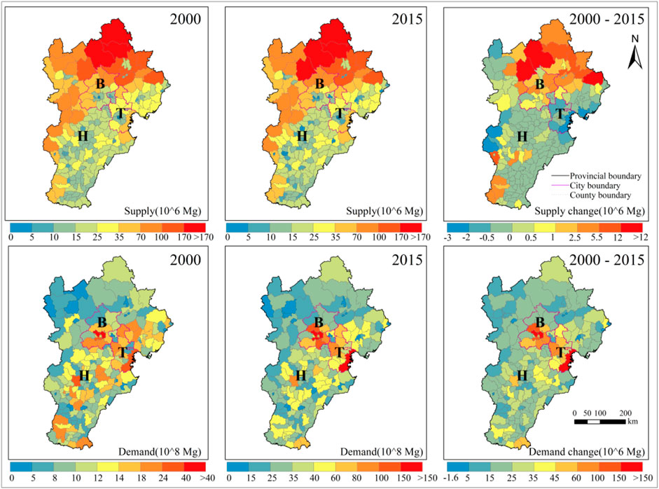
FIGURE 3. Distribution of carbon storage supply, demand and their changes from 2000 to 2015. B: Beijing city; T: Tianjin city; H: Hebei province.

Water provision

The water provision supply grew from 62.02 billion m³ in 2000 to 66.05 billion m³ in 2015—an increase of 6.49% (Supplementary Table S5). In the meantime, the demand for water decreased by 5.31%, from 2.98 × 10⁴ billion m³ in 2000 to 2.83 × 10⁴ billion m³ in 2015 (Supplementary Table S6). The area with the largest supply mainly occurs in the northern parts of the study area, followed by the western area. Areas with high demand are more concentrated in the urban built-up areas (Figure 4). From 2000 to 2015, the increases in supply mainly occurred in the northern part of the study area, while the decrease mainly occurred in the southern part. The increase in water provision service demand was mainly located in Beijing and Tianjin cities.

FIGURE 4

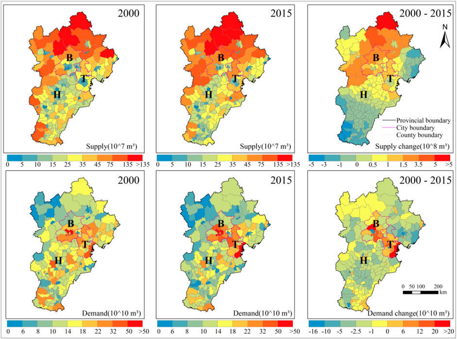
FIGURE 4. Distribution of water provision supply, demand and their changes from 2000 to 2015. B: Beijing city; T: Tianjin city; H: Hebei province.

Food provision

Food provision supply increased by 23.7%, from 4.02 million tons in 2000 to 4.97 million tons in 2015 (Supplementary Table S5). In the same period, food demand showed an increase of 25.44%, from 32.33 billion tons consumed in 2000 to 40.55 billion tons consumed in 2015 (Supplementary Table S6). The area with higher supply was Hebei Province, especially in the northwestern and southeastern parts. Beijing and Tianjin had a lower supply in 2000 and 2015 (Figure 5). From 2000 to 2015, the increases in supply mainly occurred in more counties of Hebei Province, while the food provision supply decreased sharply in Beijing and Tianjin. In terms of demand, most county scale units in Beijing and Tianjin had a markedly higher consumption than that of the counties in Hebei Province. The distribution of the increase in food provision demand was mainly located in Beijing and Tianjin cities.

FIGURE 5

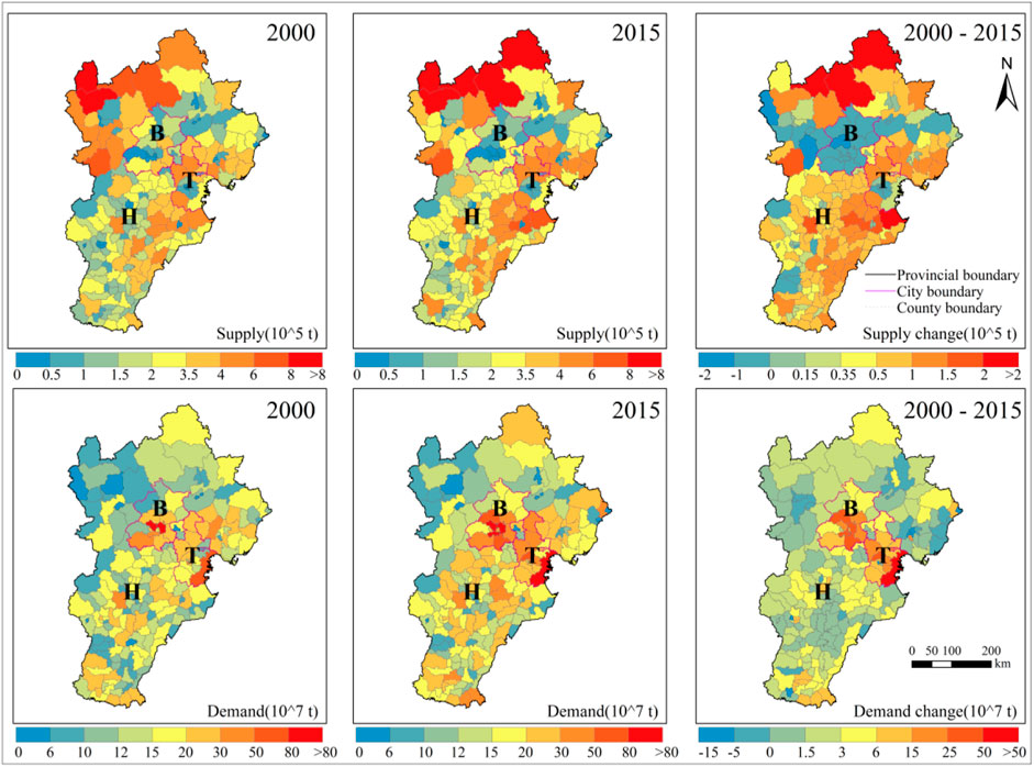
FIGURE 5. Distribution of food provision supply, demand and their changes from 2000 to 2015. B: Beijing city; T: Tianjin city; H: Hebei province.

Soil conservation

Soil conservation supply increased by 0.54% from 17.20 billion tons in 2000 to 17.29 billion tons in 2015 (Supplementary Table S5). In the same period, the demand for soil conservation showed a decrease of 22.01%, from 42.82 million tons to 33.40 million tons (Supplementary Table S6). Higher supply was mainly located in the northeastern parts of the study area, while areas with high demand were more concentrated in the southeast regions (Figure 6). From 2000 to 2015, the increases in supply mainly occurred in the northwest and northeast of Hebei Province and north and west of Beijing, while the southeast of the study area experienced a slight decrease. The distribution of the higher demand is more concentrated in the northern part of Hebei Province in 2000 and 2015. The distribution of the increase in soil conservation demand was mainly located in the southeast regions.

FIGURE 6

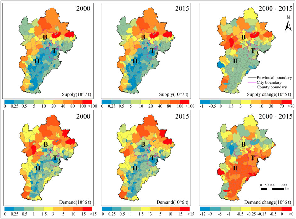
FIGURE 6. Distribution of soil conservation supply, demand and their changes from 2000 to 2015. B: Beijing city; T: Tianjin city; H: Hebei province.

Spatiotemporal changes of the ES ESDRs

Sub-area statistical analysis showed that supply-demand ESs of carbon storage, water provision and food provision services in all administrative counties and districts showed negative balances. All sub-areas were at a serious deficit over time in the BTH urban agglomeration (ESDRs <0, detailed mismatch results can be seen in Supplementary Table S7). Soil conservation was the exception; the ESDR was over 0, and showed an upward trend from 2000 to 2015. This indicates that the supply and demand of soil conservation are nearly balanced (Supplementary Table S7).

The spatial correlation of the ESDRs of ESs can be expressed by the global Moran’s I at the county or district scale using GeoDA software (Zhang et al., 2017) (Figure 7). The results showed that the global Moran’s I values increased from 2000 to 2015 for all the ES ESDRs, with their values all exceeded 0.24. High-value areas tend to be concentrated and low-value areas tend to be adjacent, indicating that the ESDRs generally present significant positive spatial correlation (Moran’s I value >0; p-value < 0.01). According to the Moran’s I scatterplot, the values for the ESDRs of carbon storage, water provision and food provision services were mainly distributed in the third quadrant, while the values for soil conservation were mainly distributed in the first quadrant (Figure 7). According to the LISA map of the ESDRs, the northern part (mainly in Hebei province) and central part (mainly in Beijing and Tianjin Municipalities) of the BTH showed a diametrically opposite spatial distribution, with the ESDRs in the northern parts showing “High-High” clustering, and the central and southeastern parts showing “Low-Low” clustering.

FIGURE 7

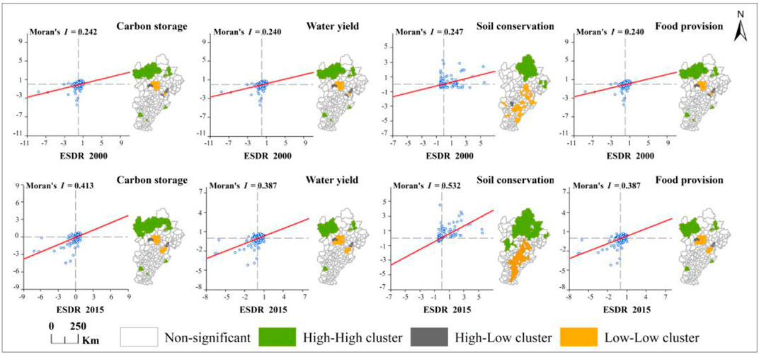
FIGURE 7. The Moran scatterplot and LISA cluster graphs of the ESDRs of four ESs in the BTH from 2000 to 2015.

Associating ESDR with driving factors

Effects the driving factors on ESDRs of ESs

The joint and individual effects of driving factors on ESDRs were analyzed using the Geodetector model (Supplementary Table S8). The results showed that the interaction effect (q) of annual average temperature (TEM) and actual evapotranspiration (EVA) changes on carbon storage, water provision and food provision was the greatest from 2000 to 2015. The next most relevant factors were average annual precipitation (PRE) and population density (POP.Den). Per capita gross domestic product (Per.GDP) interacted strongly with changes in PRE, percentage of forest land (FOR), and POP.Den. In addition, the interaction between mean slope (SLO) and TEM exhibited the largest effect on soil conservation. Soil conservation was also impacted, though not as strongly, by changes in the percentage of built-up land (BLP), changes in average annual precipitation (PRE), and changes in per capita gross domestic product (Per.GDP). The q statistics between the 11 independent variables and the ESDRs of four ESs were estimated (Table 2). Per capita gross domestic product (Per.GDP) had the largest effects on ESDR changes in carbon storage, water provision and food provision. Population density (POP.Den), percentage of built-up land (BLP), and average annual precipitation (PRE), respectively, had the next most significant effect on these ESs. The mean slope (SLO) was the most able to explain the ESDR of soil conservation, followed by mean relief amplitude (REL) and mean elevation (ELE) (Table 2).

TABLE 2

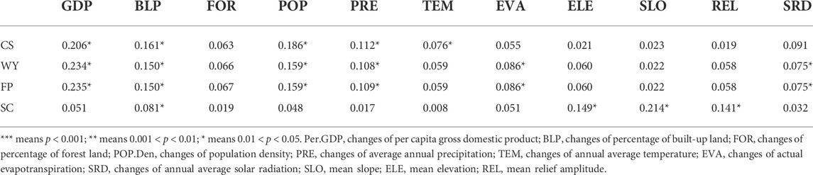
TABLE 2. The q statistics for the explanatory variables derived from Geographic Detector Model.

To examine the directional associations between the driving variables and the ESDRs, redundancy analysis (RDA) was performed (Figure 8). The results showed that the first two axes explained 42.44% of the total variation. The ESDR changes of the carbon storage, water provision and food provision services were negatively influenced by socio-economic factors, including the changes in per capita gross domestic product (Per.GDP) and population density (POP.Den). Soil conservation was positively affected by geomorphological factors, of which mean slope (SLO) was the most relevant, followed by mean relief amplitude (REL) and mean elevation (ELE).

FIGURE 8

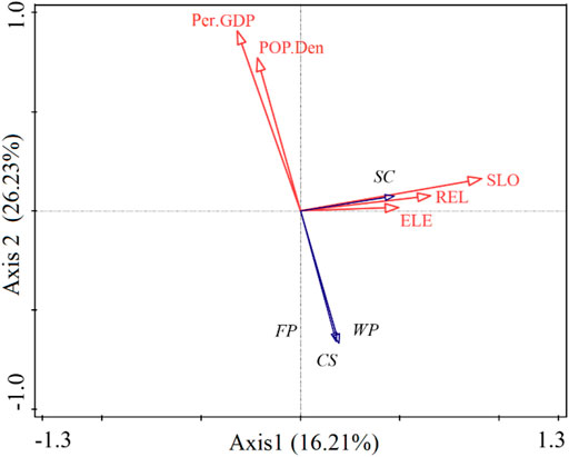
FIGURE 8. RDA results for the explanatory variables of ES ESDRs. The solid blue lines represent the ESDRs changes of ESs. The solid red lines represent the main drivers. Per.GDP, changes of per capita gross domestic product; POP.Den, changes of population density; SLO, mean slope; ELE, mean elevation; REL, mean relief amplitude.

Spatial regression between driving factors and ESDR

The spatial regression between the driving factors and ESDRs of carbon storage, water provision, food provision and soil conservation were analyzed using the MGWR model and presented in Figure 9. Anthropological factors were correlated with the ESDR changes of carbon storage, water provision and food provision, with local R² values of 0.61–0.75, 0.53–0.82, and 0.52–0.81, respectively. The low local R² value of the correlation between anthropological factors and ESDR of carbon storage was mainly distributed in the north, ranging from 0.37 to 0.46. Additionally, there is overlap in low-value areas related to water provision and food provision. These are mainly distributed in the south and east of the study area, and range from 0.11 to 0.33. While examining the spatial association between the geomorphological factors and ESDR change of soil conservation, high local R² values (R² = 0.42–0.46) were found in the eastern areas, while very low regression values (R² = 0.23–0.26) were estimated in the southern areas (Table 3). The MGWR estimates revealed that among the 11 driving factors, the anthropological factors produced were the most closely associated with the ESDR change of food provision, characterized by a maximum local R² value (R_Adj.² = 0.537).

FIGURE 9

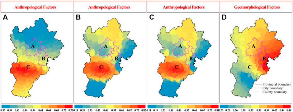
FIGURE 9. The spatial interaction between the driving factors and ESDR of (A) carbon storage, (B) water provision (C) food provision and (D) soil conservation. B: Beijing city; T: Tianjin city; H: Hebei province.

TABLE 3

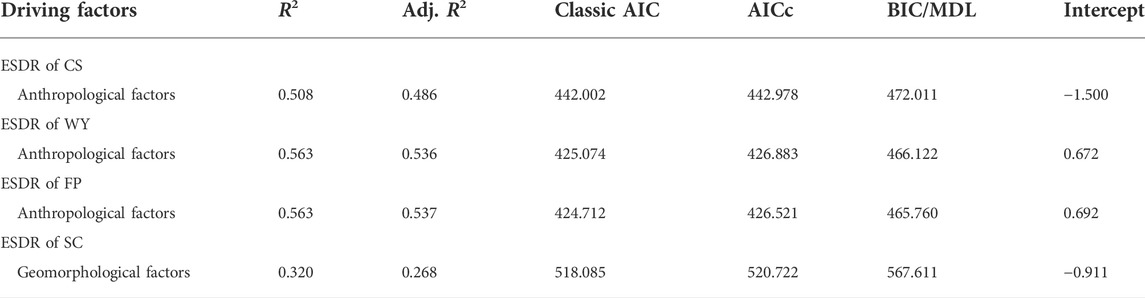
TABLE 3. MGWR statistics based on six explanatory factors, VIF based filtered factors, and all explanatory factors for different ecosystem services.

Discussion

Influencing factors of the imbalance between ES supply and demand

The BTH urban agglomeration is composed of two municipalities under the central government and 11 prefecture-level cities. The patterns of the supply and demand of ESs and ESDRs present different spatial distribution characteristics; ES supply and demand has obvious negative spatial correlations, and the spatial imbalance is prominent. This finding is inconsistent with the results discerned by (Wu et al., 2018). (Wu et al., 2018) adopted the scoring matrix method proposed by (Zhang et al., 2004) to quantify the relationship between ES supply and demand, making the scale more detailed. Areas with the lower ESDR values indicate that the ES supply and demand are extremely mismatched, and are mainly distributed in the central urban areas of Beijing and Tianjin. This is because these areas have high levels of urban economic development, high population density, and increasing demand for natural resources (Ou et al., 2018). In addition, the northern region is a key ecological area, and it is also the core of ES supply for carbon storage, water provision and soil conservation in the whole urban agglomeration. Demand in the north is, however, very low.

The shortages and mismatches of ES supply and demand are a result of the complex interaction and comprehensive influence of multiple factors including socioeconomic development and natural occurrences (Sun et al., 2019; Peng et al., 2020; Zhang et al., 2021). Geodetector model results showed that the interaction between the changes of annual average temperature (TEM) and changes of actual evapotranspiration (EVA) has the greatest influence on the ESDR changes of carbon storage, water provision and food provision, although their individual influence is very weak. Studies have shown that several climatic factors (e.g. temperature, precipitation, evapotranspiration) can have significant impacts on multiple ESs, which is illustrated also in our study (Bryan et al., 2018; Chiabai et al., 2018; Chaplin-Kramer et al., 2019; Sannigrahi et al., 2020). (Nelson et al., 2013) suggested that climate change will modify the capability of different key ecosystem functions, including food production, wildfire regulation, hazard reduction, coastal flood protection, water supply, nature-based tourism, and other recreational services. When it comes to the individual influence of factors, strong associations between anthropological factors and carbon storage, water provision and food provision were observed, which is consistent with several previous studies (Yahdjian et al., 2015; Zhang et al., 2021). This indicates that anthropological factors are important in influencing the mismatch between ES supply and demand, even though natural factors determine the mismatch from the supply side to some extent.

The mismatch of soil conservation was mainly affected by the mean slope (SLO), indicating that geomorphological factors played the dominant role; that is, supply determines the mismatch of soil conservation. This is mainly due to the calculation of ESDR of soil conservation service, which does not consider social and economic factors such as population density. Furthermore, the MGWR model was performed to evaluate the spatial interaction between the driving factors and ESDRs of carbon storage, water provision, food provision and soil conservation in the BTH region. The result showed that the anthropological influences on the ESDR of carbon storage varies with geographical space. The corresponding anthropological factors produced very high local R² values in the south-central region while they displayed lower regression estimates in the northern region. This suggests that the area near the northern forest is less vulnerable to human activities than the southern plain area.

Suggestions to balance the supply and demand for ESs

Four suggestions were put forward for the BTH urban agglomeration based on our results, which would alleviate the continuous imbalance between ES supply and demand and contribute to the sustainable development of the human-environment system. First, we recommend coordinating the spatial mismatches from both the supply and the demand sides of ESs. More attentions should be paid to alleviating the population pressure, as our study indicated that ESDRs of carbon storage, water provision and food provision are most strongly correlated with anthropological factors (Per.GDP and POP.Den) (Zhang et al., 2021). Second, from the perspective of increasing the supply of carbon storage and water provision, ecological protection and restoration should be carried out on the natural land (Yang et al., 2019). Policies aimed at reducing ES demand are unavoidable, because it is unrealistic to increase vegetated areas to meet the human demand for carbon storage. For instance, energy efficiency should be improved, and energy-saving measures should be implemented, so as to mitigate the imbalance between the supply and demand of carbon storage. Third, the spatial imbalance between ES supply and demand may trigger a series of unintended environmental concerns and social equity issues. Maintaining and improving the original ecosystem supply capacity could alleviate the contradiction between ES supply and demand (Verhagen et al., 2017; Sun et al., 2019), but it may not be the best solution, as the ecosystem has a limited capacity. On the other hand, the shortage of ESs can also be solved through trade, transportation and other measures (Cumming Cramon, 2018). For instance, food and water resources may be transferred from places further away to the urban agglomeration city center, as the area of nearby cultivated land declines and the population within the cities increases (Yu et al., 2021). In addition, implementing the consumption reduction mechanism is a more promising way to meet human demand (Kehoe and Rhodes, 2013).

Limitations and future research directions

Within the background of this study, it is difficult to comprehensively analyze all types and processes of ecosystem supply and demand, as the coupled system integrating human and natural factors is very complicated. Therefore, there are some limitations in our evaluation of ES supply and demand that need to be further explored in future studies. First, the evaluation method of ES supply is based on the land use classifications and the biophysical table, which contains the model information corresponding to each land use type and is revised according to the actual situation in BTH urban agglomeration. However, the classification standards of land use types may be different; some minor lands are considered homogeneous (Li et al., 2020; Sharp et al., 2020). Thus, the calculation of ES supply was considered inaccurate, and the regional difference characteristics of the ES supply pattern cannot be precisely described. Second, this study mainly used the socioeconomic data at the county scale to quantify the demand for ESs, which reflects spatial differences on a coarse scale. This study did not consider the conditions of different ES characteristics and local stakeholders, who may have short-term or long-term interests in ESs (Zhang et al., 2021). Therefore, in the future, we could comprehensively explore the quantification of ESs supply and demand from multiple scales and multiple stakeholders. Third, in addition to accounting for the ES supply and demand, it is important to identify who provides these ESs, which areas have the right to consume, and whether the scope of supply and consumption is available only within an area or extends to other regions (Xu et al., 2021). Even with a study that analyzes those factors, the reality of ES circulation within the regional socioeconomic system is likely more complicated than we can capture. Thus, future research is suggested to incorporate ES flow identifications into ES assessment, which will reveal more details about the interactions between the natural and social systems and provide more information on ES management (Syrbe and Walz, 2012; Schirpke et al., 2019).

Conclusion

This study explored spatiotemporal changes of ES supply and demand, as well as their mismatches in the BTH urban agglomeration of China from 2000 to 2015. Then, we focused on exploring the spatial effects of anthropological, climatic, and geomorphological factors. We further proposed several strategies to offset ES deficits. The results showed that ES supply decreased from 2000 to 2015, while ES demand increased, leading to mismatches spatially, especially in highly urbanized metropolises. To offset the ES deficits, alleviating the population pressure, protecting natural land, and implementing the energy-saving measures would be useful strategies. The anthropological factors, including Per.GDP and POP.Den, are the key drivers in the imbalance of carbon storage, water provision and food provision. Geomorphological factors, including mean elevation (ELE) and mean slope (SLO), are the key drivers for soil conservation. In addition, the drivers of ESs exhibited spatial heterogeneity. The high local R² values for ESDR changes of carbon storage, water provision and food provision are mainly distributed in the central and southern region, while a strong association for soil conservation is mainly obtained in the eastern regions. In order to alleviate ES deficits and support ES sustainability, corresponding land-use strategies and socioeconomic and ecological management measures should be adopted. Overall, more localized and efficient land-use decisions and ES management strategies should be implemented to achieve regional sustainability.

Data availability statement

The raw data supporting the conclusions of this article will be made available by the authors, without undue reservation.

Ethics statement

Ethical review and approval was not required for the study on human participants in accordance with the local legislation and institutional requirements. Written informed consent for participation was not required for this study in accordance with the national legislation and the institutional requirements.

Author contributions

Conceptualization, Methodology, and Writing-original draft, ZL; Formal analysis, BH; Valida-tion and Resources, YQ; Software and Data curation, ZL; Project administration and Supervision, BH; Visualization, YQ.

Funding

This research was funded by the Special fund project of Development Planning Office of Beijing Forestry University (2019SHFWYL02).

Acknowledgments

We would like to thank Elizabeth Tokarz at Yale University for her assistance with English language and grammatical editing.

Conflict of interest

The authors declare that the research was conducted in the absence of any commercial or financial relationships that could be construed as a potential conflict of interest.

Publisher’s note

All claims expressed in this article are solely those of the authors and do not necessarily represent those of their affiliated organizations, or those of the publisher, the editors and the reviewers. Any product that may be evaluated in this article, or claim that may be made by its manufacturer, is not guaranteed or endorsed by the publisher.

Supplementary material

The Supplementary Material for this article can be found online at: https://www.frontiersin.org/articles/10.3389/fenvs.2022.955876/full#supplementary-material

References

Ahmad, M. A., Waqar, I., Muhammad, S., Ashfaq, R., Abdul, C., Chandio, A. A., et al. (2020). Estimating dynamic interactive linkages among urban agglomeration, economic performance, carbon emissions, and health expenditures across developmental disparities. Sustain. Prod. Consum. 26, 239–255. doi:10.1016/j.spc.2020.10.006

CrossRef Full Text | Google Scholar

Anselin, L. (1995). Local indicators of spatial association-LISA. Geogr. Anal. 27, 93–115. doi:10.1111/j.1538-4632.1995.tb00338.x

CrossRef Full Text | Google Scholar

Anselin, L. (1996). “The Moran scatterplot as an ESDA tool to assess local instability in spatial association,” in Spatial analytical perspectives on GIS in environmental and socio-economic Sciences. Editors M. Fischer, H. Scholten, and D. Unwin. 1st ed. (London, UK: Taylor & Francis), 4, 111–125.

Google Scholar

Baró, F., Palomo, I., Zulian, G., Vizcaino, P., Haase, D., and Gómez-Baggethun, E. (2016). Mapping ecosystem service capacity, flow and demand for landscape and urban planning: A case study in the barcelona metropolitan region. Land Use Policy 57, 405–417. doi:10.1016/j.landusepol.2016.06.006

CrossRef Full Text | Google Scholar

Bateman, I. J., Harwood, A. R., Mace, G. M., Watson, R. T., Abson, D. J., Andrews, B., et al. (2013). Bringing ecosystem services into economic decision-making: Land use in the United Kingdom. Science 341, 45–50. doi:10.1126/science.1234379

PubMed Abstract | CrossRef Full Text | Google Scholar

Beijing Municipal Bureau Statistics (2015). From january to july, the total revenue of zhongguancun demonstration zone increased by 1.2% year-on-year. Available online: http://tjj.beijing.gov.cn/ (Accessed on July 8, 2021).

Google Scholar

Boithias, L., Acuña, V., Vergoñós, L., Ziv, G., Marcé, R., and Sabater, S. (2014). Assessment of the water supply: Demand ratios in a mediterranean basin under different global change scenarios and mitigation alternatives. Sci. Total Environ. 470, 567–577. doi:10.1016/j.scitotenv.2013.10.003

PubMed Abstract | CrossRef Full Text | Google Scholar

Borrelli, P., Robinson, D. A., Panagos, P., Lugato, E., Yang, J. E., Alewell, C., et al. (2020). Land use and climate change impacts on global soil erosion by water (2015-2070). Proc. Natl. Acad. Sci. U. S. A. 117, 21994–22001. doi:10.1073/pnas.2001403117

PubMed Abstract | CrossRef Full Text | Google Scholar

Bryan, B. A., Ye, Y., Zhang, J. E., and Connor, J. D. (2018). Land-use change impacts on ecosystem services value: Incorporating the scarcity effects of supply and demand dynamics. Ecosyst. Serv. 32, 144–157. doi:10.1016/j.ecoser.2018.07.002

CrossRef Full Text | Google Scholar

Burkhard, B., Crossman, N., Nedkov, S., Petz, K., and Alkemade, R. (2013). Mapping and modelling ecosystem services for science, policy and practice. Ecosyst. Serv. 4, 1–3. doi:10.1016/j.ecoser.2013.04.005

CrossRef Full Text | Google Scholar

Burkhard, B., Kroll, F., Nedkov, S., and Müller, F. (2012). Mapping ecosystem service supply, demand and budgets. Ecol. Indic. 21, 17–29. doi:10.1016/j.ecolind.2011.06.019

CrossRef Full Text | Google Scholar

Chaplin-Kramer, R., Sharp, R. P., Weil, C., Bennett, E. M., Pascual, U., Arkema, K. K., et al. (2019). Global modeling of nature’s contributions to people. Science 366, 255–258. doi:10.1126/science.aaw3372

PubMed Abstract | CrossRef Full Text | Google Scholar

Chen, J. Y., Jiang, B., Bai, Y., Xu, X. B., and Alatalo, J. M. (2019). Quantifying ecosystem services supply and demand shortfalls and mismatches for management optimisation. Sci. Total Environ. 650, 1426–1439. doi:10.1016/j.scitotenv.2018.09.126

PubMed Abstract | CrossRef Full Text | Google Scholar

Chiabai, A., Quiroga, S., Martinez-Juarez, P., Higgins, S., and Taylor, T. (2018). The nexus between climate change, ecosystem services and human health: Towards a conceptual framework. Sci. Total Environ. 635, 1191–1204. doi:10.1016/j.scitotenv.2018.03.323

PubMed Abstract | CrossRef Full Text | Google Scholar

Costanza, R., Arge, R., De Groot, R., Farber, S., Hannon, B., Limburg, K., et al. (1997). The value of the world's ecosystem services and natural capital. Nature 387, 253–260. doi:10.1038/387253a0

CrossRef Full Text | Google Scholar

Costanza, R., de Groot, R., Braat, L., Kubiszewski, I., Fioramonti, L., Sutton, P., et al. (2017). Twenty years of ecosystem services: How far have we come and how far do we still need to go? Ecosyst. Serv. 28, 1–16. doi:10.1016/j.ecoser.2017.09.008

CrossRef Full Text | Google Scholar

Cruz-Garcia, G., Sachet, E., Blundo-Canto, G., Vanegas, M., and Quintero, M. (2017). To what extent have the links between ecosystem services and human well-being been researched in Africa, Asia, and Latin America? Ecosyst. Serv. 25, 201–212. doi:10.1016/j.ecoser.2017.04.005

CrossRef Full Text | Google Scholar

Cui, F. Q., Tang, H. P., Zhang, Q., Wang, B. J., and Dai, L. W. (2019). Integrating ecosystem services supply and demand into optimized management at different scales: A case study in hulunbuir, China. Ecosyst. Serv. 39, 100984. doi:10.1016/j.ecoser.2019.100984

CrossRef Full Text | Google Scholar

Cumming, G. S., and Cramon-Taubadel, S. V. (2018). Linking economic growth pathways and environmental sustainability by understanding development as alternate social–ecological regimes. Proc. Natl. Acad. Sci. U. S. A. 115, 9533–9538. doi:10.1073/pnas.1807026115

PubMed Abstract | CrossRef Full Text | Google Scholar

Daily, G. C., Polasky, S., Goldstein, J., Kareiva, P. M., Mooney, H. A., Pejchar, L., et al. (2009). Ecosystem services in decision making: Time to deliver. Front. Ecol. Environ. 7, 21–28. doi:10.1890/080025

CrossRef Full Text | Google Scholar

de Groot, R. S., Alkemade, R., Braat, L., Hein, L., and Willemen, L. (2010). Challenges in integrating the concept of ecosystem services and values in landscape planning, management and decision making. Ecol. Complex. 7, 260–272. doi:10.1016/j.ecocom.2009.10.006

CrossRef Full Text | Google Scholar

Delphin, S., Escobedo, F. J., Abd-Elrahman, A., and Cropper, W. P. (2016). Urbanization as a land use change driver of forest ecosystem services. Land Use Policy 54, 188–199. doi:10.1016/j.landusepol.2016.02.006

CrossRef Full Text | Google Scholar

Deng, C. X., Liu, J. Y., Liu, Y. J., Li, Z. W., Nie, X. D., Hu, X. Q., et al. (2021). Spatiotemporal dislocation of urbanization and ecological construction increased the ecosystem service supply and demand imbalance. J. Environ. Manag. 288, 112478. doi:10.1016/j.jenvman.2021.112478

PubMed Abstract | CrossRef Full Text | Google Scholar

Fotheringham, A. S., Yang, W. B., and Kang, W. (2017). Multiscale geographically weighted regression (mgwr). Ann. Am. Assoc. Geogr. 107, 1247–1265. doi:10.1080/24694452.2017.1352480

CrossRef Full Text | Google Scholar

Fu, B. P. (1981). On the calculation of the evaporation from land surface (in Chinese). Chin. J. Atmos. Sci. 5, 23–31.

Google Scholar

González-García, A., Palomo, I., González, J. A., López, C. A., and Montes, C. (2020). Quantifying spatial supply-demand mismatches in ecosystem services provides insights for land-use planning. Land Use Policy 94, 104493. doi:10.1016/j.landusepol.2020.104493

CrossRef Full Text | Google Scholar

Hebei Municipal Bureau Statistics (2015). hebei.gov. Available online: http://tjj.hebei.gov.cn/hetj/tjsj/ (Accessed on July 6, 2021).

Google Scholar

Kareiva, P., Tallis, H., Ricketts, T. H., Daily, G. C., and Polasky, S. (2011). Natural capital: Theory and practice of mapping ecosystem services. 1st ed. Oxford, UK: Oxford University, 3–128.

Google Scholar

Kehoe, P., and Rhodes, S. (2013). Pushing the conservation envelope through the use of alternate water sources. J. Am. Water Works Assoc. 105, 46–50. doi:10.5942/jawwa.2013.105.0026

CrossRef Full Text | Google Scholar

Larondelle, N., and Lauf, S. (2016). Balancing demand and supply of multiple urban ecosystem services on different spatial scales. Ecosyst. Serv. 22, 18–31. doi:10.1016/j.ecoser.2016.09.008

CrossRef Full Text | Google Scholar

Legendre, P., and Legendre, L. F. (2012). “Multiscale analysis: Spatial eigenfunctions,” in Numerical ecology. Editors P. Legendre, and L. F. Legendre. 2nd ed. (Amsterdam, Netherlands: Elsevier), Vol. 24, 859–906.

CrossRef Full Text | Google Scholar

Legendre, P., Oksanen, J., and ter Braak, C. J. F. (2011). Testing the significance of canonical axes in redundancy analysis. Methods Ecol. Evol. 2, 269–277. doi:10.1111/j.2041-210x.2010.00078.x

CrossRef Full Text | Google Scholar

Li, D., Wu, S., Liu, L., Liang, Z., and Li, S. (2017). Evaluating regional water security through a freshwater ecosystem service flow model: A case study in beijing-tianjian-hebei region, China. Ecol. Indic. 81, 159–170. doi:10.1016/j.ecolind.2017.05.034

CrossRef Full Text | Google Scholar

Li, J., Zhang, C., and Zhu, S. (2021). Relative contributions of climate and land-use change to ecosystem services in arid inland basins. J. Clean. Prod. 298, 126844. doi:10.1016/j.jclepro.2021.126844

CrossRef Full Text | Google Scholar

Li, Z. Z., Cheng, X. Q., and Han, H. R. (2020). Future impacts of land use change on ecosystem services under different scenarios in the ecological conservation area, beijing, China. Forests 11, 584. doi:10.3390/f11050584

CrossRef Full Text | Google Scholar

Liu, L., Liu, C., Wang, C., and Li, P. (2019). Supply and demand matching of ecosystem services in loess hilly region: A case study of lanzhou. Acta Geogr. Sin. 74, 1921–1937.

Google Scholar

Mehring, M., Ott, E., and Hummel, D. (2018). Ecosystem services supply and demand assessment: Why social-ecological dynamics matter. Ecosyst. Serv. 30, 124–125. doi:10.1016/j.ecoser.2018.02.009

CrossRef Full Text | Google Scholar

Minin, E. D., Soutullo, A., Bartesaghi, L., Rios, M., Szephegyi, M. N., and Moilanen, A. (2017). Integrating biodiversity, ecosystem services and socio-economic data to identify priority areas and landowners for conservation actions at the national scale. Biol. Conserv. 206, 56–64. doi:10.1016/j.biocon.2016.11.037

CrossRef Full Text | Google Scholar

Ministry of Natural and Resources of R.P.C (MNRC) (2021). Current land use classification. GB/T21010-2017. Available online (Accessed on June 8, 2021).

Google Scholar

Mooney, H., Larigauderie, A., Cesario, M., Elmquist, T., Hoegh-Guldberg, O., Lavorel, S., et al. (2009). Biodiversity, climate change, and ecosystem services. Curr. Opin. Environ. Sustain. 1, 46–54. doi:10.1016/j.cosust.2009.07.006

CrossRef Full Text | Google Scholar

Mouchet, M. A., Lamarque, P., Martı´n-Lo´pez, B., Crouzat, E., Gos, P., Byczek, C., et al. (2014). An interdisciplinary methodological guide for quantifying associations between ecosystem services. Glob. Environ. Change 28, 298–308. doi:10.1016/j.gloenvcha.2014.07.012

CrossRef Full Text | Google Scholar

Nelson, E. J., Kareiva, P., Ruckelshaus, M., Arkema, K., Geller, G., Girvetz, E., et al. (2013). Climate change’s impact on key ecosystem services and the human well-being they support in the US. Front. Ecol. Environ. 11, 483–893. doi:10.1890/120312

CrossRef Full Text | Google Scholar

Nelson, E., Mendoza, G., Regetz, J., Polasky, S., Tallis, H., Cameron, D. R., et al. (2009). Modeling multiple ecosystem services, biodiversity conservation, commodity production, and tradeoffs at landscape scales. Front. Ecol. Environ. 7, 4–11. doi:10.1890/080023

CrossRef Full Text | Google Scholar

Onaindia, M., de Manuel, M. I., Madariaga, I., and Rodríguez-Loinaz, G. (2013). Co-benefits and trade-offs between biodiversity, carbon storage and water flow regulation. For. Ecol. Manag. 289, 1–9. doi:10.1016/j.foreco.2012.10.010

CrossRef Full Text | Google Scholar

Ou, W. X., Wang, H. N., and Tao, Y. (2018). A land cover-based assessment of ecosystem services supply and demand dynamics in the Yangtze River Delta region. Acta eco. Sin. 38, 6337e6347. (In Chinese). doi:10.5846/stxb201707061225

CrossRef Full Text | Google Scholar

Ouyang, Z., Fan, P., and Chen, J. (2016). Urban built-up areas in transitional economies of southeast asia: Spatial extent and dynamics. Remote Sens. 8, 819. doi:10.3390/rs8100819

CrossRef Full Text | Google Scholar

Peng, J., Tian, L., Liu, Y., Zhao, M., Hu, Y., and Wu, J. (2017). Ecosystem services response to urbanization in metropolitan areas: Thresholds identification. Sci. Total Environ. 607-608, 706–714. doi:10.1016/j.scitotenv.2017.06.218

PubMed Abstract | CrossRef Full Text | Google Scholar

Peng, J., Wang, X., Liu, Y., Zhao, Y., Xu, Z. H., Zhao, M. Y., et al. (2020). Urbanization impact on the supply-demand budget of ecosystem services: Decoupling analysis. Ecosyst. Serv. 44, 101139. doi:10.1016/j.ecoser.2020.101139

CrossRef Full Text | Google Scholar

Rao, Y., Zhou, M., Ou, G., Dai, D., Zhang, L., Zhang, Z., et al. (2018). Integrating ecosystem services value for sustainable land-use management in semi-arid region. J. Clean. Prod. 186, 662–672. doi:10.1016/j.jclepro.2018.03.119

CrossRef Full Text | Google Scholar

Sannigrahi, S., Zhang, Q., Pilla, F., Joshi, P. K., Basu, B., Keesstra, S., et al. (2020). Responses of ecosystem services to natural and anthropogenic forcings: A spatial regression based assessment in the world's largest mangrove ecosystem. Sci. Total Environ. 715, 137004. doi:10.1016/j.scitotenv.2020.137004

PubMed Abstract | CrossRef Full Text | Google Scholar

Schirpke, U., Candiago, S., Egarter Vigl, L., Jäger, H., Labadini, A., Marsoner, T., et al. (2019). Integrating supply, flow and demand to enhance the understanding of interactions among multiple ecosystem servicesow and demand to enhance the understanding of interactions among multiple ecosystem services. Sci. Total Environ. 651, 928–941. doi:10.1016/j.scitotenv.2018.09.235

PubMed Abstract | CrossRef Full Text | Google Scholar

Schmidt, K., Martín-López, B., Phillips, P. M., Julius, E., Makan, N., and Walz, A. (2019). Key landscape features in the provision of ecosystem services: Insights for management. Land Use Policy 82, 353–366. doi:10.1016/j.landusepol.2018.12.022

CrossRef Full Text | Google Scholar

Sharp, R., Tallis, H. T., Ricketts, T., Guerry, A. D., Wood, S. A., Chaplin-Kramer, R., et al. (2020). InVEST 3.8.0 user’s guide. The natural capital project. Stanford University, University of Minnesota. The Nature Conservancy, and World Wildlife FundAvailable online: http://releases.naturalcapitalproject.org/invest-userguide/latest/#supporting-tools.

Google Scholar

Shen, J., Li, S., Liang, Z., Liu, L., Li, D., and Wu, S. (2020). Exploring the heterogeneity and nonlinearity of trade-offs and synergies among ecosystem services bundles in the Beijing-Tianjin-Hebei urban agglomeration. Ecosyst. Serv. 43, 101103. doi:10.1016/j.ecoser.2020.101103

CrossRef Full Text | Google Scholar

Šmilauer, P., and Lepš, J. (2014). Multivariate analysis of ecological data using Canoco 5. 2nd ed. Cambridge, UK: Cambridge University, 15–38.

Google Scholar

Sun, X., Tang, H., Yang, P., Hu, G., Liu, Z. H., and Wu, J. G. (2019). Spatiotemporal patterns and drivers of ecosystem service supply and demand across the conterminous United States: A multiscale analysis. Sci. Total Environ. 703, 135005. doi:10.1016/j.scitotenv.2019.135005

PubMed Abstract | CrossRef Full Text | Google Scholar

Syrbe, R. U., and Walz, U. (2012). Spatial indicators for the assessment of ecosystem services: Providing, benefiting and connecting areas and landscape metrics. Ecol. Indic. 21, 80–88. doi:10.1016/j.ecolind.2012.02.013

CrossRef Full Text | Google Scholar

Tallis, H., and Polasky, S. (2009). Mapping and valuing ecosystem services as an approach for conservation and natural-resource management. Ann. N. Y. Acad. Sci. 1162, 265–283. doi:10.1111/j.1749-6632.2009.04152.x

PubMed Abstract | CrossRef Full Text | Google Scholar

Tang, H. J., and Li, Z. M. (2012). Study on per capita grain demand based on Chinese reasonable dietary pattern. Sci. Agric. Sin. 45, 2315–2327.

Google Scholar

The Common International Classification of Ecosystem Services (2021). cices.eu. Available online: https://cices.eu/resources/ (accessed on March 6, 2021).

Google Scholar

Tianjin Municipal Bureau Statistics (2015). State council information. Available online: http://stats.tj.gov.cn/ (Accessed on July 9, 2021).

Google Scholar

Verhagen, W., Kukkala, A. S., Moilanen, A., van Teeffelen, A. J. A., and Verburg, P. H. (2017). Use of demand for and spatial flow of ecosystem services to identify priority areas. Conserv. Biol. 31, 860–871. doi:10.1111/cobi.12872

PubMed Abstract | CrossRef Full Text | Google Scholar

Wang, J. F., Li, X. H., Christakos, G., Liao, Y. L., Zhang, T., Gu, X., et al. (2010). Geographical detectors-based health risk assessment and its application in the neural tube defects study of the Heshun region, China. Int. J. Geogr. Inf. Sci. 24, 107–127. doi:10.1080/13658810802443457

CrossRef Full Text | Google Scholar

Wang, J. F., Zhang, T. L., and Fu, B. J. (2016). A measure of spatial stratified heterogeneity. Ecol. Indic. 67, 250–256. doi:10.1016/j.ecolind.2016.02.052

CrossRef Full Text | Google Scholar

Wei, H., Fan, W., Wang, X., Lu, N., Dong, X., Zhao, Y., et al. (2017). Integrating supply and social demand in ecosystem services assessment: A review. Ecosyst. Serv. 25, 15–27. doi:10.1016/j.ecoser.2017.03.017

CrossRef Full Text | Google Scholar

Wilkerson, M. L., Mitchell, M. G. E., Shanahan, D., Wilson, K. A., Ives, C. D., Lovelock, C. E., et al. (2018). The role of socio-economic factors in planning and managing urban ecosystem services. Ecosyst. Serv. 31, 102–110. doi:10.1016/j.ecoser.2018.02.017

CrossRef Full Text | Google Scholar

Wu, A., Zhao, Y., Shen, H., Qin, Y., and Liu, X. (2018). Spatio-temporal pattern evolution of ecosystem service supply and demand in beijing-tianjin-hebei region. J. Ecol. Rural Environ. 34, 968–975. (In Chinese).

Google Scholar

Xu, Q., Yang, R., Zhuang, D., and Lu, Z. L. (2021). Spatial gradient differences of ecosystem services supply and demand in the Pearl River Delta region. J. Clean. Prod. 279, 123849. doi:10.1016/j.jclepro.2020.123849

CrossRef Full Text | Google Scholar

Yahdjian, L., Sala, O. E., and Havstad, K. M. (2015). Rangeland ecosystem services: Shifting focus from supply to reconciling supply and demand. Front. Ecol. Environ. 13, 44–51. doi:10.1890/140156

CrossRef Full Text | Google Scholar

Yang, Y., Zheng, H., Kong, L., Huang, B., Xu, W., and Ouyang, Z. (2019). Mapping ecosystem services bundles to detect high- and low-value ecosystem services areas for land use management. J. Clean. Prod. 225, 11–17. doi:10.1016/j.jclepro.2019.03.242

CrossRef Full Text | Google Scholar

Yu, H. J., Xie, W., Sun, L., and Wang, Y. T. (2021). Identifying the regional disparities of ecosystem services from a supply-demand perspective. Resour. Conservation Recycl. 169, 105557. doi:10.1016/j.resconrec.2021.105557

CrossRef Full Text | Google Scholar

Zhang, D., Huang, Q., He, C., and Wu, J. (2017). Impacts of urban expansion on ecosystem services in the beijing-tianjin-hebei urban agglomeration, China: A scenario analysis based on the shared socioeconomic pathways. Resour. Conservation Recycl. 125, 115–130. doi:10.1016/j.resconrec.2017.06.003

CrossRef Full Text | Google Scholar

Zhang, L., Hickel, K., Dawes, W. R., Chiew, F. H. S., Western, A. W., and Briggs, P. R. (2004). A rational function approach for estimating mean annual evapotranspiration. Water Resour. Res. 40, 2. doi:10.1029/2003wr002710

CrossRef Full Text | Google Scholar

Zhang, Z., Peng, J., Xu, Z. H., Wang, X. Y., and Meersmans, J. (2021). Ecosystem services supply and demand response to urbanization: A case study of the pearl river delta, 49. China: Ecosystem Services, 101274.

CrossRef Full Text | Google Scholar

Zuur, A. F., Ieno, E. N., Walker, N. J., Saveliev, A. A., and Smith, G. (2009). Mixed effects models and extensions in ecology with R. 1st ed. New York, USA: Springer, 323–341.

CrossRef Full Text | Google Scholar