K-textures, a self-supervised hard clustering deep learning algorithm for satellite image segmentation

Deep learning self-supervised algorithms that can segment an image in a fixed number of hard clusters such as the k-means algorithm and with an end-to-end deep learning approach are still lacking. Here, we introduce the k-textures algorithm which provides self-supervised segmentation of a 4-band image (RGB-NIR) for a k number of classes. An example of its application on high-resolution Planet satellite imagery is given. Our algorithm shows that discrete search is feasible using convolutional neural networks (CNN) and gradient descent. The model detects k hard clustering classes represented in the model as k discrete binary masks and their associated k independently generated textures, which combined are a simulation of the original image. The similarity loss is the mean squared error between the features of the original and the simulated image, both extracted from the penultimate convolutional block of Keras “imagenet” pre-trained VGG-16 model and a custom feature extractor made with Planet data. The main advances of the k-textures model are: first, the k discrete binary masks are obtained inside the model using gradient descent. The model allows for the generation of discrete binary masks using a novel method using a hard sigmoid activation function. Second, it provides hard clustering classes–each pixel has only one class. Finally, in comparison to k-means, where each pixel is considered independently, here, contextual information is also considered and each class is not associated only with similar values in the color channels but with a texture. Our approach is designed to ease the production of training samples for satellite image segmentation and the k-textures architecture could be adapted to support different numbers of bands and for more complex self-segmentation tasks, such as object self-segmentation. The model codes and weights are available at https://doi.org/10.5281/zenodo.6359859.

1 Introduction

In recent years, automatic extraction of cartographic features from satellite images is undergoing a revolution thanks to advances brought by deep convolutional neural networks (CNNs). The main advantage of these supervised CNNs is that they take raw data and automatically learn features through training with minimal prior knowledge about the task (LeCun et al., 1998). Furthermore, CNN accuracy in remote sensing applications is similar to human-level classification accuracy, but is consistent and fast, enabling rapid application over very large areas and/or through time (Brodrick et al., 2019). CNNs could support the fast acquisition of accurate spatial information about land use and land cover change, which is essential for country planning and monitoring. However, among the most significant efforts that are being made to map Land Use and Land Cover (LULC) such as the project MapBiomas, which maps LULC change specifically for Brazil (MapBiomas, 2018) or Global Forest Change product at 30 m spatial resolution of the University of Maryland (Hansen et al., 2013), the CNNs are still under-used and semantic classifications rely mostly on machine learning (ML) algorithms, such as the random forest algorithm.

The use of supervised CNN techniques for these remote sensing applications is limited by their need for large training samples labeled by experts. Making manual samples, and even dense labeling (each pixel attributed to a label) is feasible in sub-metric spatial resolution images where objects such as buildings or trees are visible. However, this is more difficult and inaccurate for small objects at high or medium spatial resolution (5–30 m resolution) satellite imagery, such as Planet, Sentinel, or Landsat, which are typically used for LULC change mapping at regional to global scales. As consequence, manual sampling is generally made of spatial referenced points with labels determined either with high-resolution imagery or in the field. These sets of points are used to train machine learning (ML) algorithms, such as Random Forest, and to validate classification results. After the training step, in prediction, a class is attributed to each pixel of the satellite image scene. The classification process assumes that pixels are spatially independent. To improve the spatial coherence of the prediction, additional temporal filters are used to improve the classification. For example, a pixel labeled as a forest cannot switch labels and then become a forest again (Souza et al., 2020). Having unsupervised methods that could automatically generate dense samples for one or several land cover classes would ease the laborious manual part of the mapping and enable to make a large number of samples to train supervised CNNs and ML segmentation techniques.

Several classical unsupervised algorithms are used to produce semantic segmentation in remote sensing classification of medium spatial resolution images such as k-means, ISOSeg, Maximum Likelihood, Mahalanobis Distance, and Bhattacharyya Distance (Richards and Richards, 1999; Câmara et al., 2008). However, they are not accurate enough to replace the manual labeling approach. This is easy to understand since they rely on clustering pixels with similar values in the color channels, without considering spatial information of the neighbor pixels, or considering spatial information with texture indices, which is oversimplistic. For example, values in the spectral bands (or values in the color channels red, green, and blue) can be seen as one feature when we currently know that several features and multiple levels of abstraction are needed to reach state-of-the-art accuracy of classification (LeCun et al., 2015), as demonstrated by the success of CNNs in computer vision tasks. Furthermore, while for natural object color is an important feature, as it links structural and chemical composition (Asner et al., 2015; Ferreira et al., 2016), for most of the non-natural objects, the color is most of the time an undesirable feature. For example, to recognize cars or plastic balloons in images, color is not the most helpful feature, and often the CNN models are even trained with images where the hue is artificially changed (during data augmentation) to impede the model to give too much importance to the color, that is, overfitting, and to improve generalization (Chollet and Allaire, 2018). However, all these non-CNN classical unsupervised algorithm techniques are still used for classifying the high to medium spatial resolution satellite imagery because developing deep learning equivalent of these unsupervised methods for image segmentation is a current challenge. Furthermore, specifically, to map LULC changes in tropical regions, the community has now free access to the Planet images, which are multispectral satellite cloud-free images at a spatial resolution (5 m) and a monthly temporal resolution (Planet Team, 2017; Planet, 2021). However, the Planet images are recent, the monthly dataset started in September 2020, and few reference datasets exist for these images. Today, because of the large amount of freely available satellite data and the growing need for sample production for supervised techniques, an unsupervised deep learning approach for segmentation would greatly benefit the community.

Unsupervised deep learning is seen as the future of deep learning, as this is mostly how humans and animals learn, by observations (LeCun et al., 2015; Bengio et al., 2021). This field of research has gained interest in the last years, and the term “self-supervision” is now preferred to “unsupervised” because the model creates its own abstraction of objects. Self-supervised image segmentation, in remote sensing or computer vision, is currently one of the most challenging tasks for deep learning. Recent works show that self-supervised deep learning models can be trained in a way that semantic information emerges directly inside the features of the model such as the self-supervised Vision Transformer (Caron et al., 2021). Other attempts to automatically segment images have used Variational Autoencoder (VAE) or simpler CNNs to produce the features and used k-means clustering on the features created by the algorithm to provide pseudo labels (Girard et al., 2019; Kim et al., 2020). Finally, the last method is redrawing, where the model extracts an object’s mask and redraws the object at the same location (Chen et al., 2019). However, all of these unsupervised segmentation techniques, and more generally all the models of clustering with deep learning (Karim et al., 2021), belong to soft clustering, that is, every pixel has a probability or likelihood to belong to each of the clusters. Clusters are obtained by the argmax function on the softmax layer of the object class but are not used directly inside the model during optimization, as the argmax function is non-differentiable. Alternatively, Fard et al. (2020) have developed an unsupervised technique to simultaneously train a representation model and the associated soft clusters that can provide, in some conditions, hard clusters but the model has a specific loss function which contains the cluster number and limits the use of other loss functions. If we had true binary masks used as a weight inside the model, textures or images could be generated for each cluster independently and with a loss function independent of the number of clusters k.

By contrast, in hard clustering, the pixels belong or do not to the cluster, 0 or 1. This problem of discretization using gradient descent is currently not known to be solvable by deep learning because it is impossible currently to compute the gradient for discrete search. In other words, having a function that returns 0 or 1 (or more generally a step function) is discrete and non-differentiable and is not optimized by current gradient-based deep learning techniques. However, here, we present a simple technique to avoid this limitation, and to render a discrete search possible, that is, in our case, to assign a hard cluster to each class and use it in the gradient computation but without disrupting the gradient descent. There have been some works on the binarization of the weights in the deep learning field (Qin et al., 2020) and some very close to the methods used here (Sakr et al., 2018; Courbariaux et al., 2015). However, the objective of these works was to build lighter and more computationally efficient networks, not to use directly the binary weights as labels to provide the segmentation of an image.

Our model is called k-textures as it self-segments the image in k hard clustering classes of different textures. As a study case, it was tested for self-semantic segmentation of a cloud-free RGB-NIR 20 km × 20 km Planet satellite image at 4.78 m of spatial resolution covering a degraded region of the Amazon forest in Brazil. The planet images over the tropics image have been made available by Norway’s International Climate and Forest Initiative (NICFI, https://www.nicfi.no/) (Planet Team, 2017). The results of k-textures were compared to the results obtained by k-means, which is the closest nondeep learning machine learning algorithm for clustering images. Furthermore, we compare the obtained classes to the real world in land cover types obtained from MapBiomas (2018) to understand the capabilities and limitations of the k-textures model.

2 Proposed K-textures model

2.1 Hard sigmoid activation function with a very steep linear part

The objective of this section is to create a differentiable function that can return a binary value of 0 or 1 from a continuous value, to create a binary mask for each k class of the model. A step function that returns only 0 or 1 from a continuous input variable is not differentiable and, thus, not usable in deep learning with gradient descent optimization. However, a differentiable function that returns 0 or 1 for most of the input values should exist. The hard sigmoid function is amongst the functions that are differentiable and used as an activation function in deep learning and has this characteristic. The hard sigmoid function σ(x) was originally defined in Eq. 1 (Courbariaux et al., 2015) and Figure 1. The function is composed of three connected parts, one that is constant and equal to 0, one that is linear and rises from zero to 1, and a final part, constant and equal to 1. For example, in Tensorflow (https://www.tensorflow.org/api_docs/python/tf/keras/activations/hard_sigmoid) (Abadi et al., 2016) the hard sigmoid function tf.keras.activations.hard_sigmoid return 0 if x $<$ −2.5, return 1, if x $>$ 2.5 and if −2.5 $<=$ x $<=$ 2.5: return 0.2 × x + 0.5, Eq. 2 and Figure 1. The coefficients of the hard sigmoid function can be adjusted so that the slope can occur in a very limited range of x values. In other words, the coefficients can be set so that the function returns as y constant values of 0 or 1 on most of the x values range and only returns y values on the range (0,1) on a very narrow range of x values, with the advantage that the function remains differentiable. For example, in our hard sigmoid activation function, we use the coefficients of Eq. 3 which constrain the linear part that rises from 0 to 1 between x values of 0 and 0.0002 and Figure 1.

${\sigma }_{\mathit{Courbariaux}}\left(x\right)=\max \left(0,\min \left(1,x\times 0.5+0.5\right)\right)(1)$

${\sigma }_{\mathit{Tensorflow}}\left(x\right)=\max \left(0,\min \left(1,x\times 0.2+0.5\right)\right)(2)$

${\sigma }_{\mathit{ours}}\left(x\right)=\max \left(0,\min \left(1,x\times 5000+0\right)\right).(3)$

FIGURE 1

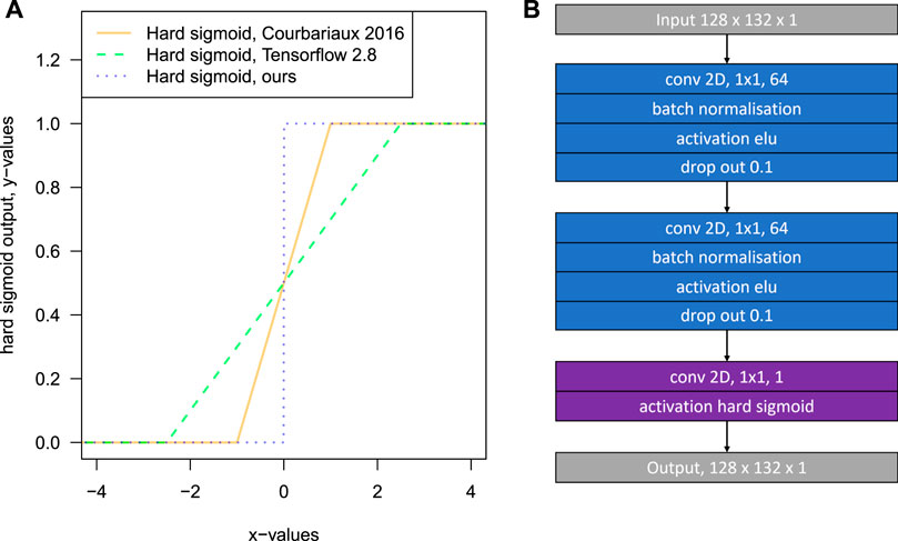
FIGURE 1. Hard sigmoid curves for x values ranging between −4 and 4 for the function of Courbariaux et al. (2015), Tensorflow 2.8 (Abadi et al., 2016) and our function where the linear part rises from 0 to 1 for x values between 0 and 0.0002 in panel (A). Panel (B): Architecture of the hard sigmoid approximation σ_CNN model. Note that all the convolution layers have kernels of 1 × 1 indicating that each value is independent of the neighbors.

2.2 A CNN to approximate the hard sigmoid function

As using the hard sigmoid function with such a steep slope directly inside a CNN would be unstable, and, to ease the convergence, the hard sigmoid function was approximated by a CNN. This enables to decomposed of the hard sigmoid function in an ensemble of small and easy to differentiate operations. To train a CNN that is able to approximate our hard sigmoid function, we build a small CNN architecture (σ_CNN) and simulated the data to train the model, Figure 1B, Figure 2 and Eqs 4–11. This CNN model is used to generate dummy variables for k categories inside the k-textures model. Using a CNN allows us to decompose our problem in a series of small linear operations that can be easily used as a layer with fixed weights inside a larger deep learning model, to transform continuous data into categorical data while still enabling the use of gradient descent optimization. The architecture of the hard sigmoid CNN model (σ_CNN) is presented in Figure 1B. The model is made of two convolution blocks with 64 filters a and 1 × 1 kernel, both consisting of the application of a 2D convolution layer, batch normalization, elu activation, and dropout. Dropout was used to perform further implicit data augmentation and avoid overfitting during training. Finally, the output is produced with a final 2D convolution layer with 1 × 1 kernel, 1 filter, and our custom hard sigmoid activation function (Section 2.1).

FIGURE 2

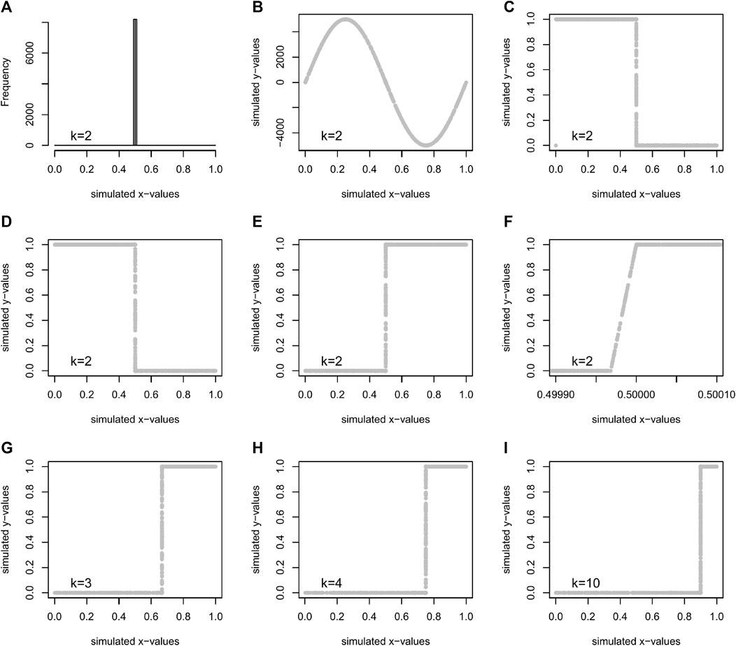
FIGURE 2. Data generated for training a CNN (σ_CNN) to approximate the hard sigmoid function with k classes. The frequency of the simulated x values (Eqs 5, 6) for k = 2 (A), simulated sin function from the simulated x values with Eq. 7 (B), clipped values on the range [0,1] Eq. 8 (C), y value different of 1 set to 1 for x value near 0 9 (D), inversion along x for even k classes, Eq. 10, and y value different of 1 are set to 1 for x value near 1, Eq. 11, to obtain the final y value used to train the model for a number of classes k = 2 (E), details of the linear part where y rise from 0 to 1 (F), examples of data simulated to train the model for a number of k classes of 3 (G), 4 (H) and 10 (I).

The simulated input and output data to train the model were built with the functions described in Eqs 4–11, where k is the number of classes, k_threshold is the x values located at the end of the rising linear part where y reaches the value of 1, x_sim are the simulated input values y_sim are the simulated output values and U a random uniform distribution for n samples ranging from a defined minimum and maximum value. Input values were sampled from three uniform distributions with differences in frequency, that is, most of the input values (96.97%) were sampled in a random uniform distribution located in the linear part of the curve, Eq. 5. For the two other distributions, the same number of values were simulated on each side of the linear part of the hard sigmoid curve to ease convergence, Eq. 5. All the simulated input values in the interval [−0.001,1.001] were clipped to [0,1] to match the range of values returned by a sigmoid activation function and also to have data for x = 0 and x = 1.

To simulate the y value, the starting point is a sine function, Eq. 7, with a large amplitude (5,000) computed from the simulated x values normalized between −1 and 1. The result is then clipped to the interval [0, 1]. Then, test/corrections are made by applying sequentially Eqs 8–11 to ensure that y values are equal to 0 or 1 on the extremes, near x = 0 and x = 1. A sine function was used to ease the production of simulated output for different values of k classes. As a convention, we keep the constant part equal to 1 on the right, so the function is inverted along x for k classes that are even. Simulated output data for k = 2 are presented in Figures 2E,F, for k = 3 in Figure 2G, for k = 4 in Figure 2E and for k = 10 in Figure 2I.

$k_{\mathit{threshold}}=\left(k-1\right)/k(4)$

$\begin{array}{ll}\hfill x_{\mathit{sim}}& =\left(U\left(\mathit{min}=-0.001,\mathit{max}=k_{\mathit{threshold}},n=128\times 2\right),\right.\hfill \\ \hfill & \left.U\left(\mathit{min}=k_{\mathit{threshold}}-0.003,\mathit{max}=k_{\mathit{threshold}}+0.003,n=128\times 128\right)\right),\hfill \\ \hfill & U\left(\mathit{min}=k_{\mathit{threshold}},\mathit{max}=1.001,n=128\times 2)\right)\hfill \end{array}(5)$

$x_{\mathit{sim}}=clip\left(x_{\mathit{sim}},\mathrm{0,1}\right)(6)$

$y_{\mathit{sim}}=\frac{5000}{k-1}\times \sin \left(\left(\left(\frac{\pi /2}{1/k}\right)\times \left(\left(x_{\mathit{sim}}\times 2\right)-1\right)\right)\right)(7)$

$y_{\mathit{sim}}=\left\{\begin{array}{cc}0,\hfill & \text{if}{y}_{\mathit{sim}}<=0\hfill \\ 1,\hfill & \text{if}{y}_{\mathit{sim}}>=1\hfill \\ y_{\mathit{sim}},\hfill & \text{otherwise}\hfill \end{array}\right.(8)$

$y_{\mathit{sim}}=\left\{\begin{array}{cc}1,\hfill & \text{if}{x}_{\mathit{sim}}<\left(1/k\right)/2\hfill \\ y_{\mathit{sim}},\hfill & \text{otherwise}\hfill \end{array}\right.(9)$

$y_{\mathit{sim}}=\left\{\begin{array}{cc}1+\left(y_{\mathit{sim}}\times -1\right)\hfill & \text{,\hspace{0.17em}if}k\text{is\hspace{0.17em}even}\hfill \\ y_{\mathit{sim}},\hfill & \text{otherwise}\hfill \end{array}\right.(10)$

$y_{\mathit{sim}}=\left\{\begin{array}{cc}1,\hfill & \text{if}{x}_{\mathit{sim}}>1-\left(\left(1/k\right)/2\right)\hfill \\ y_{\mathit{sim}},\hfill & \text{otherwise}\hfill \end{array}\right.(11)$

The hard sigmoid approximation σ_CNN model for each k class was trained with 16,384 images of 128 × 132 × 1 that represent 276824064 simulated x values and their correspondent simulated y value. All x and y were simulated again at each epoch. The model σ_CNN was trained for 5,000 epochs with a batch size of 1,024. During network training, we used a standard stochastic gradient descent (SGD) optimization with a learning rate of 0.0001. The loss function was designed as a sum of two terms: binary cross-entropy and the Dice coefficient-related loss. The model with the minimum mean absolute error was chosen. If the linear part that rises from 0 to 1 of the curve produced by the CNN was in the interval ±0.0001 around the value 1–1/k, the desired accuracy was achieved and the training was stopped. Otherwise, the training continued for 5,000 more epochs until the accuracy was attained (and repeated if necessary). The training of the model with k = 16 and 5,000 epochs took approximately 27 min using a Nvidia RTX2080 Graphics Processing Unit (GPU) with an 8 GB memory.

The hard sigmoid approximation (σ_CNN) model with fixed weights corresponding to the k class is used during the generation of the binary masks for each class in the k-texture model. For example, for k = 3 classes, the three binary masks can be computed with σ_CNN for an input whose values are in the range [0,1], as presented in Figure 3. The range [0,1] corresponds to the values returned by the convolution layer with a sigmoid activation function and here the example is given for input values on the range [0,1] with a uniform distribution, Figure 3A. The first binary mask is computed by applying the σ_CNN model directly on the input value, Figure 3B. The second binary mask is obtained by applying the σ_CNN model to the (1 - input value), Figure 3C. The third binary mask is computed by removing the sum of the two previously obtained masks to a tensor the same size as the mask, filled with 1, Figure 3D. The sum of the three masks is a tensor of ones. The operation to produce the binary masks can be generalized to any desired number of classes with a simple operation on the input values and the obtained intermediate masks (code available at https://doi.org/10.5281/zenodo.6359859). Note that the values in the masks can be different from 0 or 1 if an x value is located on the linear segment that rises from 0 to 1 of the hard sigmoid produced by the σ_CNN model. This issue is resolved later during the training of the k-texture model. Note that this method enables us to use the σ_CNN model to transform a continuous into a binary variable and at the same time this model can be used with gradient descent because the σ_CNN is fully differentiable.

FIGURE 3

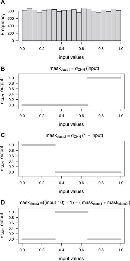
FIGURE 3. Computing binary mask values for k = 3 with our σ_CNN model which approximate a hard sigmoid function. Sample of uniform x values on the range [0,1] (A), values of the mask obtained by the binarization for mask_class1 (B), mask_class2 (C) and mask_class3 (D).

2.3 K-textures model architecture

The objective of the k-textures algorithm is to self-segment an image in k number of classes. The architecture of the k-textures algorithm is divided into two paths, Figure 4, an encoder to generate the k binary masks and an independent generator of textures. Both join before the end of the architecture to reconstruct the image.

FIGURE 4

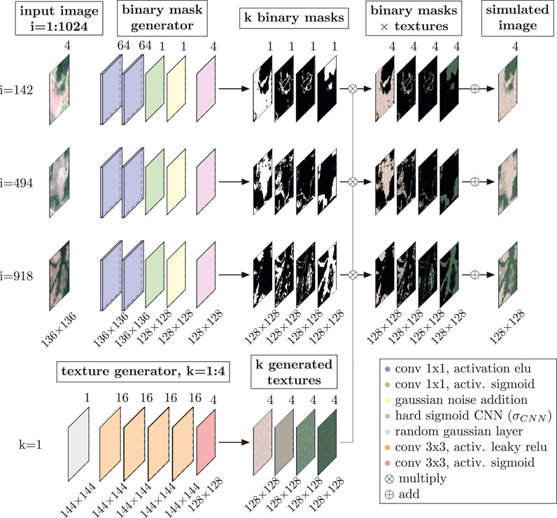
FIGURE 4. K-textures Model Architecture and example for k = 4. The Planet image (4,096 × 4,096 pixels) is inputted to the k-textures algorithm in square patches of 136 × 136 pixels with 8 pixels of overlap (1,024 patches). k binary masks are generated for each patch. One texture is generated for each k classes with the texture generator, to produce k textures of 128 × 128 pixels. Note that only k textures of 128 × 128 pixels are estimated for the entire Planet image (k = 4 in the example). The k textures and the k binary masks are then multiplied and the result summed to produce a simulate image of each patch. During the training, the loss that contains the VAE and VGG16 feature extractors is computed between the input and simulated images.

The first path of the model is an encoder where the input image goes through two convolution blocks with 64 filters and 1 × 1 kernel (2D convolution layer, batch normalization, and elu activation), and a last 2D convolutional layer which returns a tensor with sigmoid activation cropped to the size of (128,128,1), Figure 4. Kernels of 1 × 1 are used in the encoder (each pixel is independent of the other), as CNNs using a 3 × 3 kernels are already used in the feature extractor of the Loss function and there is no need to have them here (even if it is possible to use an encoder with 3 × 3 kernels). Furthermore, it enables to decrease in the number of weights and it is more comparable to the k-means models where pixels are considered independently. A Gaussian noise (mean = 0, sd = 0.0005) is added to the sigmoid activation tensor returned by the encoder, and the σ_CNN model with fixed weights corresponding to the k number of classes is applied to generate the k binary masks.

The Gaussian noise amplitude (sd = 0.0005) is slightly larger than the x value of the linear part of the σ_CNN model that rises from 0 to 1, to ensure that all x values in the linear part are significantly affected by the noise. This adds instability to the gradient during training on the risen part of the hard sigmoid so that the algorithm tends to avoid these values. For example, on one epoch the x values on the slope plus Gaussian noise can return a y value of 0 and 1 in the next epoch. With this simple Gaussian noise, the model is unable to learn the rising part of the curve and tends to avoid it because of its instability. Furthermore, and more importantly, the model is unable to use this part of the curve to propagate information, and, as a consequence, it tends to return either 0 or 1. On the other hand, the x values located on the constant part of the curve (equal to 0 or 1) are stable even with the Gaussian noise.

The second path of the model is designed to generate k textures, that is, one texture for each class. The texture is generated from a random Gaussian tensor of size (144, 144, 1). The texture is generated on a larger tensor than the original image to avoid the border effects. The random Gaussian tensor is then applied a series of four identical convolutional blocks (2D convolution layer, batch normalization, and leaky relu activation) with 16 filters and a kernel size of 3 × 3. Then a 2D convolution with 4 filters, a kernel size of 3 × 3, and a sigmoid activation are applied to produce the texture image. The generated textures are then clipped to the size of the binary masks. Finally, the two paths meet to produce the reconstructed image from the k binary masks and the k textures. Each binary mask is multiplied by its correspondent textures, and all the resulting tensors are all summed together to produce the reproduced image, the output of the model.

The model is trained with the same image as input and as the image to reproduce, the only difference is that the input is slightly larger (136 × 136) than the image to reproduce (128 × 128) to avoid border effects. As these images are patches of a larger image, the larger border for the input is obtained by overlapping the neighbor patches and when overlapping is not possible, missing input data on the border is extrapolated by mirroring. The k-texture model is designed to optimize simultaneously using gradient descent, the k textures, and the k binary masks that enable the production of an image the most similar to the original image. The model can be trained with a various number of classes and we give the weights of the σ_CNN model for the number of classes k from 2 to 64 but note that we only tested that the model works until k = 32. We used the ADAM optimizer (Kingma and Ba, 2017) with a learning rate of 0.001 and the gradient norms were scaled if the gradient vector exceeds 1. The gradient scaling helps the convergence of the model as was observed by trial and error.

For the k-textures model, we designed a loss function which is the mean square error between the feature obtained from a feature extractor on the original image (input image) and the reconstructed image (model output). It enables the model to compare the two images not only on one feature, such as the color for example but for all the different features present in the feature extractor. For the feature extractor, we use the pre-trained VGG16 model (Simonyan and Zisserman, 2014) with the fixed ImageNet weights available in Keras (Chollet et al., 2015; Allaire and Chollet, 2016), specifically, the second to last layer of the model (block5_conv3). The VGG16 feature extractor works only for RGB (3 bands) images, and, as we want to apply the model on 4 band images, we also train a custom variational autoencoder (VAE) with 130 satellites images (Planet Scope, Section 3.1) and a mean squared error (mse) loss to be further used as 4 bands image feature extractor. The VAE model was a standard U-Net model (Ronneberger et al., 2015) (https://blogs.rstudio.com/ai/posts/2019-08-23-unet/) with the input of (256 × 256 × 4) but without skip connections in the decoder part. Note that other feature extractors could be used. The fixed weight used in the k-textures loss for feature extraction was obtained after training the VAE model for 3,898 epochs when the best accuracy of the VAE model was achieved (0.9703441). The last central layer before the decoder of this VAE was used as a feature extractor. Then both feature extractors, from VGG16 and our custom VAE were used in the loss function. The loss of the k-textures model was defined as the sum of two terms: 1) the mean square error of the feature extracted with VGG16 for the input and the simulated image, and 2) the mean square error of the feature extracted by the custom VAE for the input and the simulated image. Once trained, the model with fixed weights can be eventually applied to other images. In this case, it will generate the new binary masks and use the textures obtained during training.

All the models were coded in the programming language R (R Core Team, 2016) with Rstudio interface to Keras (Chollet et al., 2015; Allaire and Chollet, 2016) and Tensorflow (Abadi et al., 2016).

3 Experiments

3.1 Planet satellite image and associated land use/cover datasets

The experiment was undertaken in a region of the Brazilian Amazon forest located in the Mato Grosso State, Brazil, and centered at 9°32′8.43″S, 59°9′1.69″W, Figure 5. The region contains several different land cover types, such as primary and secondary forests, pastures in use, and abandoned and urban areas. Furthermore, this region is currently of critical importance and at the center of international attention because of the carbon emissions due to deforestation and forest degradation. It also contains numerous small patches of forests that would be highly time-consuming to sample by hand in the high-resolution image. Furthermore, in Brazil, the land cover types and water surfaces have been already mapped by the MapBiomas initiative using Landsat satellite image at 30 m spatial resolution, enabling us to understand and compare what the clusters of the k-textures and the k-means models represent in the real world, Figure 5B.

FIGURE 5

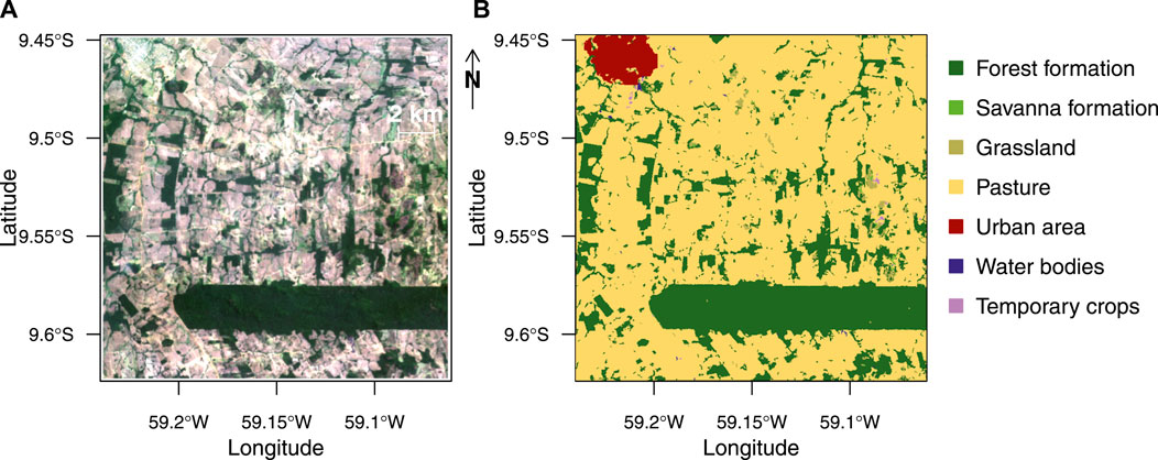
FIGURE 5. Geographical location of the region of interest with RGB composite of the Planet image used in the experiment (A); land use/cover classes of the region of interest for the year 2020 from the MapBiomas project (B).

The Planet image of 20 × 20 km at ∼ 4.78 m spatial resolution over the study region, Figure 5A, was downloaded through the Planet API https://api.planet.com/basemaps/v1/mosaics (Planet Team, 2017). The image was selected because it has a lower cloud cover among the available images of the region times series and because it did not show a visible variation of atmospheric conditions or illumination effects. The Planet ID of the image is ID_ce7bad0f-a4a0-45fd-904b-eb6cc6eee373_PAGE_687-969_DATE_2021-08-01. tif and was acquired in July 2021. We used 4 bands for this image: Red (0.650–0.682 μm), Green (0.547–0.585 μm), Blue (0.464–0.517 μm), and the NIR bands (0.846–0.888 μm) (Planet, 2021). All bands in raw image digital numbers (12 bits) were, first, truncated to the range 0–2,540 for the RGB bands and scaled between 0 and 2,540 for the NIR bands (i.e., divided by 3.937). Second, the 4 bands were scaled to 0–255 (8 bits) by dividing by 10, and then the Red-Green-Blue-NIR (RGBNIR) composite was built. The forest reflectance values are low in the RBG bands ($<$ 500) and the specific scaling of these bands was made to keep a good definition of the forest reflectance values in 8 bits. The scaling of NIR is only a min-max (0–10000) scaling as forest reflectance values are not low in this band. No atmospheric correction was performed. A second image was generated from the composite adding a mirroring border of 4 pixels on each side for the generation of input images.

The clusters obtained from the k-textures segmentation were compared to the results obtained with a k-means algorithm, which aims to partition the pixels values of the image into k groups such that the sum of squares from pixels values to the assigned cluster centers is minimized (MacQueen, 1967; Lloyd, 1982). The k-means were tested using the four reflectance bands, that is, the same dataset as for the k-textures, and for a number of k clusters from 4 to 16. Furthermore, to account for spatial information, we also apply the k-means with five texture indices (mean, variance, entropy, homogeneity, dissimilarity) in addition to the four reflectance bands of the image. These texture indices were computed with the R package glcm (Zvoleff, 2020) on the grey-level image from the RGB reflectance bands. The k-means were used with the MacQueen algorithm and a maximum number of iterations of 10.000 for convergence. Processing times for the k-means with 4 bands were 24.5 s for 4 classes, 157.0 s for 16 classes, and 518.5 s for 32 classes. Mean absolute error (MAE) was computed a posteriori between the original image and the image produced by k-means, that is, with the cluster centers used as a texture for each class. The loss of k-means for the 4-bands dataset was computed using the loss function of the k-textures model with the observed image and the image with cluster center values for each cluster.

To test if our segmentation or the k-means-based segmentation was consistent with independent datasets of land cover/use maps of the region, and if the classes seen by the k-texture model classes represent features in the real world, we compared the results to the land use/cover map from the Project MapBiomas - Collection 6 (MapBiomas, 2018), Figure 5B. MapBiomas Project is a multi-institutional initiative the to generate annual land cover and use maps using automatic classification processes applied to satellite images. A complete description of the project can be found at http://mapbiomas.org. The MapBiomas land cover classes for the year 2020 over the region study extent at 30 m spatial resolution was obtained from google earth engine https://mapbiomas.org/en/colecoes-mapbiomas-1?cama_set_language=en. The MapBiomas image was resampled to overlay exactly the Planet image spatial resolution using gdalwarp with the nearest neighbor resampling method (GDAL/OGR contributors, 2019). To compare the Mapbiomas forest class to the forest classes obtained by the k-textures and the k-means, the metrics precision, recall, accuracy, F1-score, and intersection over union (IOU) were computed.

3.2 Training

Clipping the Planet image in 136 × 136 pixels images with 4 pixels of overlap resulted in a sample set of 1,024 images to train the model. The model output is a 128 × 128 image, however, using a 136 × 136 pixels image as input enabled to avoid border effects in the encoder output when using the kernel of 3 × 3 pixels. This size of 136 × 136 pixels was selected because the main texture of the land cover and land use classes are assumed to visible in an image of that size (136 pixels ∼ 649 m) and, because of GPU memory limitation, as a larger image would need larger GPU memory. Note that, for larger GPU memory, the algorithm could be adapted. We trained our network for 15,360 epochs with a learning rate of 0.001, and where each epoch comprised 1 batch with 1,024 images for the k classes from 4 to 24 and 32. Training the model took ∼18 min for k = 4 and ∼80 min for k = 32 using GPU on an Nvidia RTX2080 with 8 GB of dedicated memory.

4 Result

4.1 Model convergence

Here, we compare the evolution of the loss value during training of 15,360 epochs with different values of k for the planet image presented in Figure 5A). The k-textures model converged as shown by the decrease of the loss during the 15,360 epochs of training for all values of k, Figure 6. The loss of the model for k of 4 is higher than expected, as with only 4 classes the model is not able to reproduce the variability of the image. For other k values, lower loss values are observed but without clear order. The model shows sometimes relatively sharp changes in loss when improving, that could be due to the reorganization of textures order or the creation of new textures/classes. The decrease in loss indicates that the model is able to train, that is, it can estimate the binary class and texture jointly to reproduce the original image.

FIGURE 6

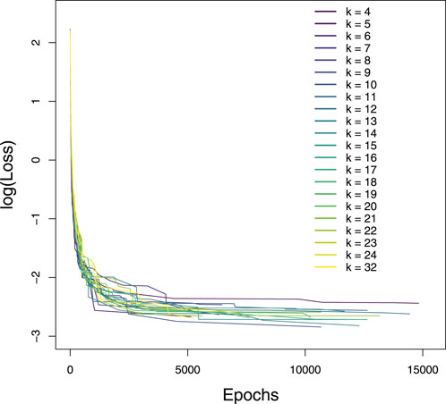
FIGURE 6. Evolution of the Feature Loss during the training of 15,360 epochs for the k considered classes, that is, from 4 to 24 and 32. The loss line stops at the best loss value for the run with 15,360 epochs and only the points with decrease in loss are represented. Loss is given in logarithmic scale to ease visualization.

The k-textures model produces a better classification than the k-mean when looking at mean average error (mae) and Loss, Table 1. The k-textures model reaches a lower mean average error (mae) with fewer k-classes when compared to k-means. For example, for 4 classes, the mae of k-textures is equivalent to the mae of 7 classes for k-means; and, for 9 classes, it already reaches the mae corresponding to 16 classes with k-means. This result was expected (and our experiments confirm it) since k-textures results involve several colors along with spatial information for one class while k-means only includes one color per class, the cluster center, that has one unique value in each of the four bands. Adding the spatial information with the texture bands in the k-means does not improve the MAE, and MAE is always above the k-means MAE and k-textures MAE on four bands. For the loss, the reconstruction of the image with simulated textures also provides a resulting image that is closer to the original image, specifically, more similar in features than the image returned by the k-mean algorithm, has shown by the lower value of loss for k-textures in Table 1. This is also expected as this is the value that the k-textures try to minimize during training. While k-means only focus on the values of pixels taken independently, the k-textures model uses CNNs and consequently multiple levels of abstraction and it can perform better.

TABLE 1

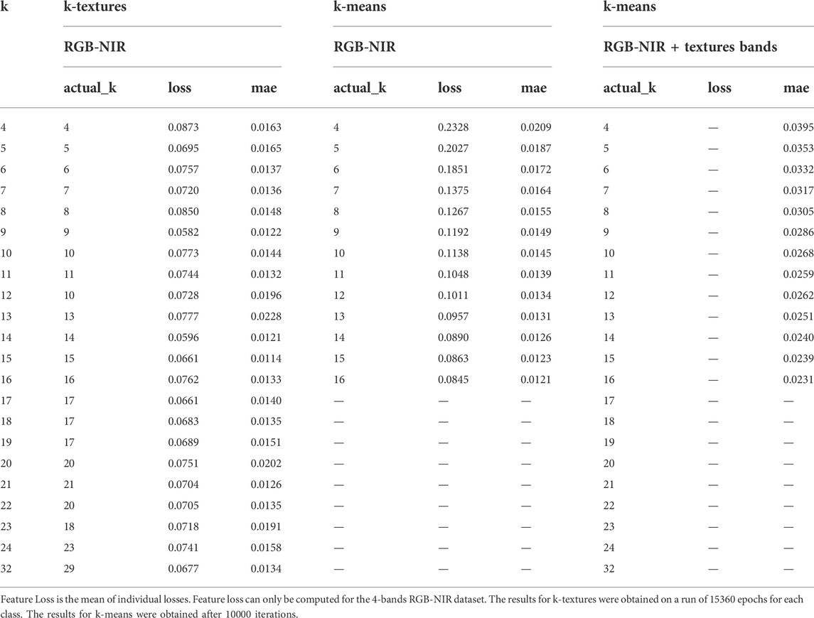
TABLE 1. Comparison between the k-textures and the k-means models of the number of clusters found (actual k), the feature loss and the mean absolute error (MAE). MAE was computed a posteriori between the original image and the image produced by k-means, that is, with the cluster centers used as texture for each class. The loss of k-means for the 4-bands dataset was computed using the loss function of the k-textures model with the observed image and the image with cluster center values for each cluster.

While for the k-means, Loss, and mae systematically improve when adding a class, the results of k-textures seem more subject to variations and to reach a limit where the model does not further improve. This effect could be related to the number of epochs, as 15,360 epochs might not be enough for a high number of groups, or other model parameters such as the batch size and learning rate. Further experiments will be needed to determine how to obtain the best model for a class. Sometimes, the k-textures model does not find the requested number of k classes. In this case, the missing clusters are always those corresponding to the extreme values of the encoder sigmoid activation value (near 0 or near 1). Finally, like the k-means, the k-textures results are always different between runs.

4.2 Binary masks

All the binary masks obtained after training for 15,360 epochs are mostly filled with 0 and 1, that is, more than 99.999% of the values, Table 2. This shows that our model produces stable binary masks that are effectively used as weights during the training with stochastic gradient descent. However, there were still a few nonbinary values and they represent a proportion ranging from 0.0000015 to 0.0004612% of the total pixels of the masks, Table 2. As the linear increasing part of the hard sigmoid returned by the σ_CNN model ranges in a maximum interval of ±0.0001 (0.0002) on the x-values. The percentage of expected values in this interval to be obtained by chance from a random distribution (ranging from 0 to 1 and with 4096² values like our tensor) will be of 0.02%. Here, the observed percentage of nonbinary values is relatively smaller than this 0.02 percent, as the max percent of non-binary values in our study is 0.0004612%. So, the model is likely avoiding the linear increase. It cannot learn this part of the hard sigmoid, but still, due to the update of weights, some weights combinations in the encoder can sometimes result by chance in a nonbinary value in the mask. So here, we acknowledge that we still cannot impede that a very limited number of values returned by the σ_CNN model for the mask are nonbinary. In our case, for self-segmentation, this is not so important, as even in the case of a nonbinary value for a pixel a unique cluster is attributed to the pixel with the argmax function. However, in further works which cannot have any non-binary values, not even a very small percentage, this might be improved by increasing the slope of the hard sigmoid estimated by the σ_CNN model.

TABLE 2

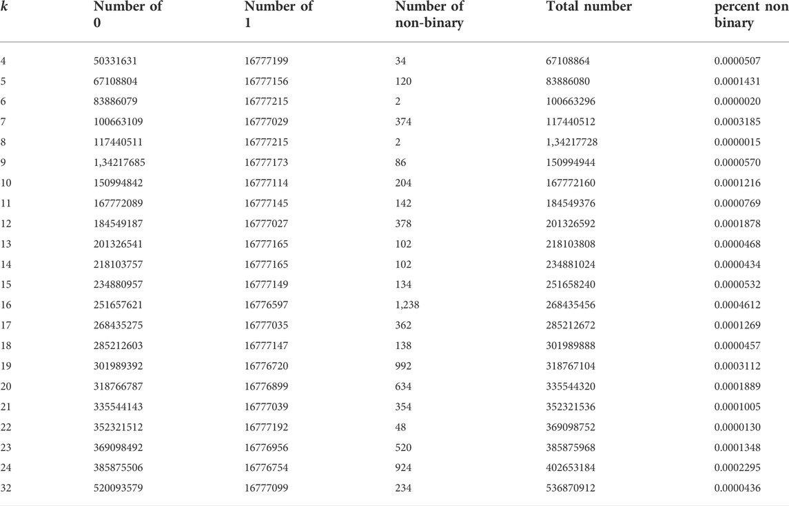
TABLE 2. Description of the values in the binary masks (0, 1 or non-binary values) which were obtained by the k-textures model for all the k classes presented in this work (from 2 to 24 and 32).

The binary masks provided by the model, for example in Figure 7, are estimated by the model and then used to multiply the corresponding textures that are also estimated simultaneously. The final reconstituted image is then the sum of all the products of the binary masks and their corresponding textures, Figure 4. A pixel of the image can have the value 1 in only one binary mask. The values in the binary masks are weights of the models. Observing Figure 7, it appears clearly that the binary mask can form a coherent spatial patterns, that is the model can estimate the weights of the mask and of the texture at the same time, inside the same neural network. This shows that under certain conditiona, here in our case the restriction of the search space to discrete search space, the CNN is able to converge even with some weights being only 0 and 1.

FIGURE 7

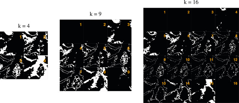
FIGURE 7. Example of binary masks obtained by the k-textures model for k = 4, 9 and 16 classes for a patch of 128 × 128 pixels extracted from the planet 4,096 × 4,096 pixels image. For k = 9 and k = 16, the patch does not contain all the clusters, it is not mandatory for a patch to contain all the clusters.

4.3 Generated textures

The k textures simulated by the k-textures model and the k colors of the cluster obtained by the k-means for k in 4, 9, and 16 are given in Figure 8. In comparison to k-means, the k-textures gives not only simple class correspondences, but also reveal the characteristic spatial patterns of textures. The textures estimated by the k textures model look natural and organic. The textures estimated for the forest, for example, are visually close to what is observed in the real images, with brighter crowns and a lot of shade. The grain is different between the obtained textures showing that our texture generator is able to simulate a variety of textures. Some textures appear with light strides but it is still not clear if this is due to the generator like it could be with GANs (Chollet and Allaire, 2018), or because this is actually better for the loss. No border effects between adjacent patches were observed when segmenting a large image, however, some light border effects sometimes appeared in the texture patches generated by the k-textures model.

FIGURE 8

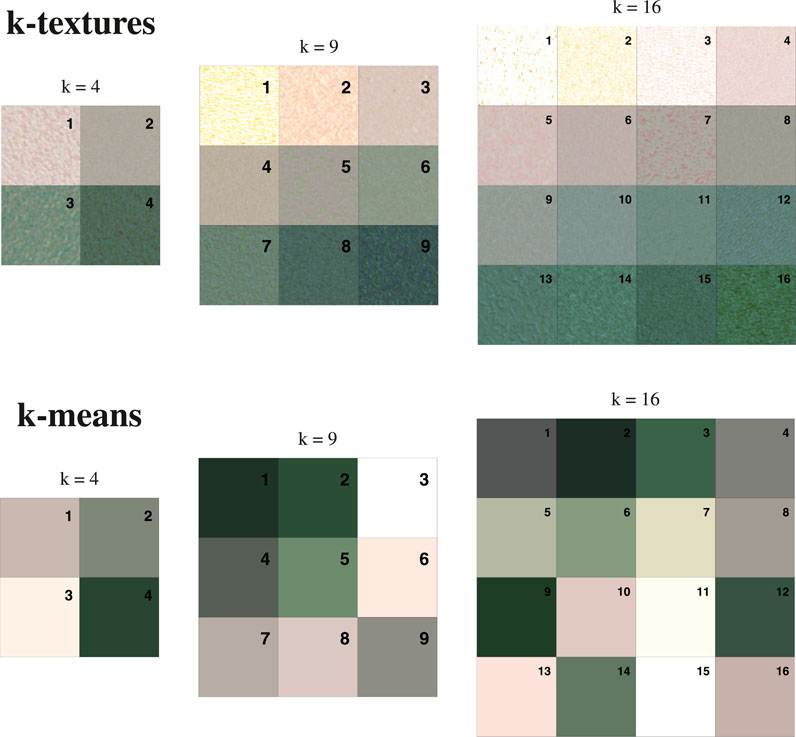
FIGURE 8. Example of the k textures simulated by the k-textures model and the colors of the cluster obtained by the k-means for k = 4, 9 and 16 classes. The matrix of textures are filled by row, starting by the top left, in the order returned by the models. Note that, for an easy visualization, only RGB bands are displayed but the estimated textures have 4 bands, RGB and NIR. For the k-textures model of 9 classes, the forests are mostly encountered in the cluster 8 and 9; the savanna, grassland and water bodies are in cluster 8, 7 and 6; and clusters lower than 5 are related to pasture and urban areas, see Table 3.

Surprisingly, the k-textures model sorts the textures, with apparently less difference between the nearby textures, and with the textures of higher hue at the opposite of the texture’s lower hue. This 1D order likely emerged from the model architecture and was unexpected. This could be due to the methods for producing the binary masks with σ_CNN, as the attribution to a class is only determined by the value ranging between 0 and 1 returned by the encoder. It seems that the model loss value is lower when textures are ordered, as this order is found for all values of k. As the encoder is a CNN, it might produce continuous variations from one class to another, and the ordered textures could reflect this. Here the RGB reflectance values in the satellite image do not show extreme variations and are relatively close (∼ terrains colors), but it could be interesting to see how the model behaves with a more complex reflectance value composition. Ordering color is a challenge in machine learning and here our algorithm manages to order the classes by textures in 1D and clustering at the same time. As a comparison, one of the best recent machine learning algorithms to represent color or classes on a 2D projection, t-SNe (Van der Maaten and Hinton, 2008), is designed to order the pixels in a 2D plane to provide a representation of the data, but not to cluster the data.

For k-means, the obtained colors are similar to those in the textures produced by the k-textures, Figure 8. No order appears as the k-means is not made for this and only searches for centroids (in 4 dimensions in our specific case). Colors with higher and lower hues are observed in the classes returned by the k-means, while, for the k-textures model, the colors with the highest or lowest hue appeared mixed in textures with other colors.

4.4 Comparison of k-textures classes with real-world land use classes from mapbiomas

The k-textures show association with the real-world land cover class from Mapbiomas, that is, most of the land cover classes are represented by a limited number of k-textures clusters, Table 3. As our model orders the textures, it renders the table easy to read and to determine which cluster corresponds to which class or to which transition between land cover classes, Table 3. For example, from the results of a k-textures model trained using 9 classes, Table 3, it can be observed that the forests are mostly in clusters 8 and 9 of the k-textures model (93.42%). Then the savanna, grassland, and water bodies are in clusters 8, 7, and 6, and clusters lower than 5 are related to pasture and urban areas. For the temporary crops, some were in the cluster of vegetation (around cluster 7) and some in clusters without vegetation or cultures and with bare soils (cluster 2). The land cover class sometimes overlaps with two or three clusters, however note that the land cover classes are made with Landsat images at 30 m spatial resolution while the Planet images used in the k-textures models have a spatial resolution of ∼4.77 m, so some overlap is expected. The forests are mostly found in the cluster 1 and 2 of the k-means model (88.37%). The table of the k-means results does not bring much visual information and seems to associate one particular color to each class, at least for the k-means computed with RGB-NIR bands, Table 3. For the k-means computed with RGB-NIR bands and the five texture bands, the Mapbiomas classes appeared more mixed between the clusters. For example, the forest class is mainly distributed in three clusters and pasture in five clusters. In our results, Table 3, the k-textures clusters are more unbalanced (0.07%–27.58%) than the k-means clusters (2.55%–18.49% for the k-means on RGB-NIR bands and 2.99%–17.5% for the k-means on RGB-NIR and texture bands) but this could be an artifact as k-means does not search for the same number of observations inside each cluster, and more investigation should be made to check if our model is able to cluster data situation not know to be easily resolved by k-means, such as when clusters are of different sizes and densities.

TABLE 3

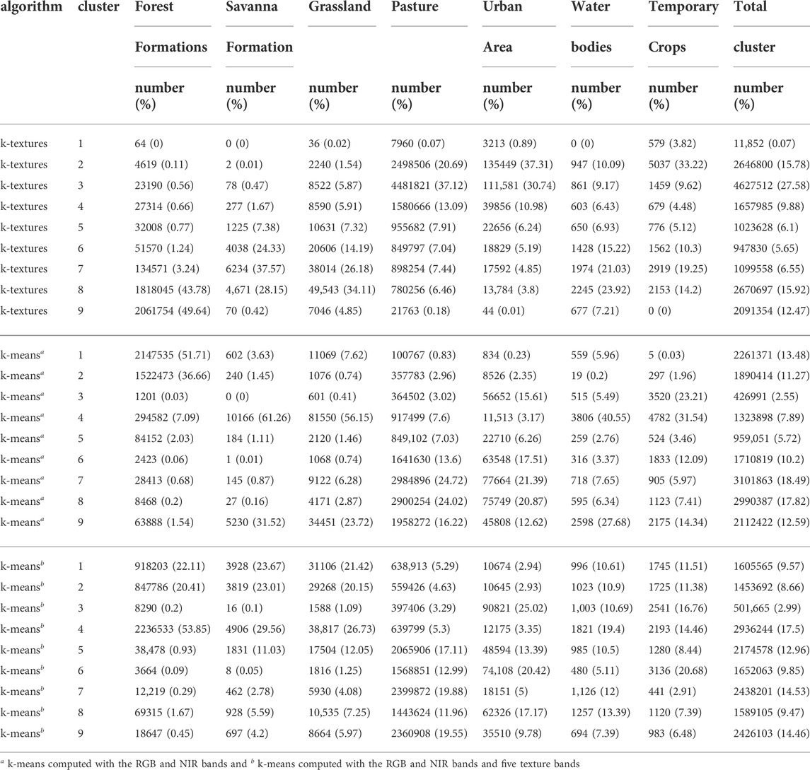
TABLE 3. Distribution of the clusters of k-textures and k-means by Mapbiomas landcover classes.

The segmentation accuracy of the forest classes is obtained by the k-textures (union of clusters 8 and 9), by the k-means (union of clusters 1 and 2), and by the k-means with the band images and the five texture indices (union of cluster 1, 2 and 4) are given in Table 4. The Mapbiomas forest mask is at 30 m spatial resolution, consequently, it is not expected that this mask contains small forests that can be segmented with the k-textures or k-means in the 5 m Planet spatial resolution, and the accuracy metrics results should be interpreted with caution. The k-means with RGB-NIR bands shown higher performance for the precision, accuracy, F1-score, and intersection over union metrics. The k-means with RGB-NIR bands and the five texture bands showed a higher performance for the recall. Finally, the k-textures model was in the second position for all performance metrics.

TABLE 4

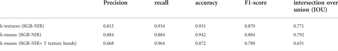
TABLE 4. Metrics of segmentation accuracy computed between the Mapbiomas forest class (reference) and the forest classes obtained with the k-textures and the k-means.

4.5 Example of tropical forest self-segmentation

In this section, the objective is to self-segment Planet satellite image with the k-textures model to produce a highly accurate training sample that could be used to train a supervised deep learning model for tropical forest mapping. Just like in k-means, the number of clusters in k-textures should be chosen manually. Finding indices to help determine the best number of k classes for the k-textures model will be addressed in future works. For instance, the user has to visually check the original versus predicted image and mask (for example Figure 9) or compare with other data sets to determine the k-number of classes that seems the best for the segmentation problem, such as the Mapbiomas land cover data. Specifically, for forests, we are searching for classification 1) with textures that reproduce the texture of the forest, 2) without much inclusion of other clusters, and 3) that does not have too many clusters on the pixel representing border or transition classes. With k = 4, Figure 9, the model included too many pixels in the cluster corresponding to forest texture. For k = 16, the segmentation does not seem to improve much when looking at the simulated image, in comparison to k = 9, and it seems there are too many clusters inside the forest. However, it can be also noted that the model finds a good texture for the forest and keep this solution with one texture while it had a lot of available classes. For forest segmentation, it can be observed that a k-textures model with k = 9 clusters already provides a good texture representation of the forest, Figure 9. Furthermore, a total of 93.42% of the pixels classified as forest by Mapbiomas are in the k-textures clusters 8 and 9, Table 3. Consequently, these two clusters, 8 and 9, were merged and used to make the forest mask, Figure 10B.

FIGURE 9

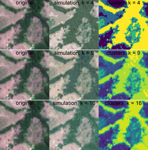
FIGURE 9. Example of the simulated image and clusters obtained with the k-textures algorithm for a number of classes k = 4, 9 and 16.

FIGURE 10

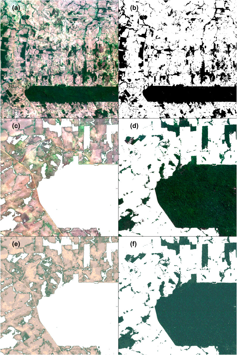
FIGURE 10. Example of self-segmentation of a Planet image using the k-textures model and k = 9 classes. Original Planet image (A), for visualization only RGB bands are used. Forest mask produced with k-textures self-segmentation (B) where clusters 8 and 9 have been interpreted by the user to be forest and other cluster to represent other land used. Planet image with colors channels set to [255,255,255] for the pixels in the forest mask (C). Planet image with colors channels set to [255,255,255] for the pixels outside the forest mask (D). Simulated Planet image from the k-textures model with colors channels set to [255,255,255] for the pixels in the forest mask (E) and Simulated Planet image from the k-textures model with colors channels set to [255,255,255] for the pixels outside the forest mask (F).

The forest mask resulting from the self-segmentation, Figure 10B, can be used directly to train a supervised model, such as a U-net model Ronneberger et al. (2015); Wagner et al. (2019). The first advantage is that it gives a class per pixel, consequently, it might be more accurate spatially than a manually drawn sample, which generally consists of manual-made polygons that are therefore rasterized which led to large inaccuracy on the pixels at the border of classes. The manual equivalent of our model would be to determine the belonging of a class for each pixel individually. It also has the advantages of the CNNs: the segmentations are fast and consistent (Kattenhorns; Kattenborn et al., 2021), and the pixel are classified using a large number of features, not only the values in the color channels. For example, the original and the simulated images are compared with the 131,072 features from the second to the last layer of the VGG16 model (block5_conv3 of size 16 × 16 × 512) and the 131,072 values of the central layer before the decoder of our custom VAE (size 16 × 16 × 512). These features are extracted at the end of the encoder for both VGG16 and the VAE model, and, consequently, they represent a high level of abstraction. To manually produce the mask given in Figure 10B would also be extremely time-consuming due to a large number of forest patches and likely not as accurate because of the large number of features used in the model which humans are unlikely to capture consistently. The main limitation of the k-textures is that it cannot consider variations that comes from atmospheric condition and shade and it can work properly only if there are little to no variation in illumination inside a class. The model does not account for the variation of texture between image patches, for example, the same texture of 128 × 128 is used for all the patches with forested pixels. To improve this in the future, the model could be adapted to account for the variability of the atmospheric condition or shade, for example, the simulated image could be the sum of the texture × classes added or multiplied to a layer of atmospheric/illumination.

Comparing the colors and textures of the original image, Figures 10C, D, and the simulated image, Figures 10E, F, it can be observed that the model enables to simulate colors and textures that appear visually, to some extent, close to the original image. Note that this is a sub-image and the texture of the simulated forest is the same used in the entire image. For the non-forest classes, the model tends to ignore the roads which are of higher hue in the original image. The colors and pattern of roads are smaller, only a few pixels, in relation to the size of the texture patch (128 × 128), so this could be why the model cannot reproduce this spatial pattern. For the forest, the simulated texture is comparable to the real forest textures, with shade and some brighter pixels that are the crowns of the trees. In the 10f, the pattern of the (128 × 128) texture patches can be seen. For the production of masks for segmentation, even the k-textures algorithm can produce extremely accurate segmentations, we recommend that the user check visually and correct the mask when necessary. For example, for forests, the model is not expected to account for large variations of features, for example, pink or yellow flowering, clouds, and dark shade.

5 Conclusion

In this work, we present the k-textures algorithm, a self-supervised algorithm that provides a per pixel self-segmentation of an image according to k number of classes. The model searches for binary masks using gradient descent, that is, the binary masks are generated and used as weights inside the algorithm. Note that some weight combinations in the encoder can result by chance in a non-binary value in the mask due to the update of weights, however in proportion below 0.0005%. The model remains continuous and fully differentiable by using methods involving the hard sigmoid function and Gaussian noise. To our knowledge, this is the first-time binary masks are produced and used as weights inside a classical CNN to produce the classes. In contrast to the current clustering method using deep learning that all belong to soft clustering, our model returns hard clusters: each pixel has only one class. These binary masks enable us to generate a texture per class inside the k-textures architecture. Our model is better than the k-means algorithm for self-segmentation because 1) it resolves the same problem, that is, hard clustering of an image in k classes but without assuming a particular distribution of the values inside the clusters and 2) it uses the capacity of the CNNs, mainly different level of abstraction and spatial context. The k-textures model generates complex textures for each class while the k-means relies on individual pixel values in the color’s channels, and/or more complex features that can contain spatial information, such as textural indices, but that has to be designed manually. The k-textures produce textures similar to the original image. Additionally, the k-textures model sorts the textures along one dimension based on their characteristics. This is likely because of the architecture of the σ_CNN model used to generate the binary masks and because it helps to decrease the loss. Finally, the hard clustering classes returned by our model can be used for self-segmentation in order to produce training sample of objects with particular texture, such as shown for dense tropical forest cover in a Planet image.

Data availability statement

Publicly available datasets were analyzed in this study. This data can be found here: https://doi.org/10.5281/zenodo.6359859.

Author contributions

Conceptualization, FW, RD, AS, and MH; methodology, FW, RD, AS, and MH; software, FW, RD, and AS; validation, FW; formal analysis, FW; investigation, FW; resources, FW; data curation, FW and RD; writing–original draft preparation, FW, RD, AS, and MH; writing–review and editing, SF, JL, SM, YY, and SS; visualization, FW; supervision, FW and SS; project administration FW and SS; funding acquisition, FW and SS.

Funding

The research leading to these results received funding from the project BIO-RED“Biomes of Brazil—Resilience, Recovery, and Diversity”, which is supported by the São Paulo Research Foundation (FAPESP, 2015/50484-0) and the United Kingdom. Natural Environment Research Council (NERC, NE/N012542/1). FW has been funded by FAPESP (grant 2016/17652-9). RD acknowledges the support of the FAPESP (grant 2015/22987-7). We also thank the Amazon Fund through the financial collaboration of the Brazilian Development Bank (BNDES) and the Foundation for Science, Technology and Space Applications (FUNCATE) no. 17.2.0536.1 (Environmental Monitoring of Brazilian Biomes). Part of this work was carried out at the Jet Propulsion Laboratory, California Institute of Technology, under a contract with the National Aeronautics and Space Administration (NASA).

Conflict of interest

The authors declare that the research was conducted in the absence of any commercial or financial relationships that could be construed as a potential conflict of interest.

Publisher’s note

All claims expressed in this article are solely those of the authors and do not necessarily represent those of their affiliated organizations, or those of the publisher, the editors, and the reviewers. Any product that may be evaluated in this article, or claim that may be made by its manufacturer, is not guaranteed, or endorsed by the publisher.

References

Abadi, M., Agarwal, A., Barham, P., Brevdo, E., Chen, Z., Citro, C., et al. (2016). Tensorflow: Large-scale machine learning on heterogeneous distributed systems. arXiv preprint arXiv:1603.04467.

Google Scholar

Allaire, J., and Chollet, F. (2016). keras: R Interface to ’Keras’. R package version 2.1.4

Google Scholar

Asner, G. P., Anderson, C. B., Martin, R. E., Tupayachi, R., Knapp, D. E., and Sinca, F. (2015). Landscape biogeochemistry reflected in shifting distributions of chemical traits in the Amazon forest canopy. Nat. Geosci. 8, 567–573. doi:10.1038/NGEO2443

CrossRef Full Text | Google Scholar

Bengio, Y., Lecun, Y., and Hinton, G. (2021). Deep learning for ai. Commun. ACM 64, 58–65. doi:10.1145/3448250

CrossRef Full Text | Google Scholar

Brodrick, P. G., Davies, A. B., and Asner, G. P. (2019). Uncovering ecological patterns with convolutional neural networks. Trends Ecol. Evol. 34, 734–745. doi:10.1016/j.tree.2019.03.006

PubMed Abstract | CrossRef Full Text | Google Scholar

Câmara, G., Vinhas, L., Ferreira, K. R., De Queiroz, G. R., De Souza, R. C. M., Monteiro, A. M. V., et al. (2008). “Terralib: An open source gis library for large-scale environmental and socio-economic applications,” in Open source approaches in spatial data handling (Springer), 247–270.

Google Scholar

Caron, M., Touvron, H., Misra, I., Jégou, H., Mairal, J., Bojanowski, P., et al. (2021). “Emerging properties in self-supervised vision transformers,” in Proceedings of the IEEE/CVF International Conference on Computer Vision, 9650–9660.

CrossRef Full Text | Google Scholar

Chen, M., Artières, T., and Denoyer, L. (2019). Unsupervised object segmentation by redrawing. Adv. neural Inf. Process. Syst. 32.

Google Scholar

Chollet, F., and Allaire, J. (2018). Deep learning with R. New York, NY: Manning Publications Co.

Google Scholar

Chollet, F., Ganger, M., Duryea, E., and Hu, W. (2015). Keras. GitHub.Available att: https://github.com/fchollet/keras.

Google Scholar

Courbariaux, M., Bengio, Y., and David, J.-P. (2015). Binaryconnect: Training deep neural networks with binary weights during propagations. Adv. neural Inf. Process. Syst. 28.

Google Scholar

Fard, M. M., Thonet, T., and Gaussier, E. (2020). Deep k-means: Jointly clustering with k-means and learning representations. Pattern Recognit. Lett. 138, 185–192. doi:10.1016/j.patrec.2020.07.028

CrossRef Full Text | Google Scholar

Ferreira, M. P., Zortea, M., Zanotta, D. C., Shimabukuro, Y. E., and de Souza Filho, C. R. (2016). Mapping tree species in tropical seasonal semi-deciduous forests with hyperspectral and multispectral data. Remote Sens. Environ. 179, 66–78. doi:10.1016/j.rse.2016.03.021

CrossRef Full Text | Google Scholar

GDAL/OGR contributors (2019). GDAL/OGR geospatial data abstraction software library. Beaverton, OR: Open Source Geospatial Foundation.

Google Scholar

Girard, N., Zhygallo, A., and Tarabalka, Y. (2019). Clusternet: Unsupervised generic feature learning for fast interactive satellite image segmentation, Image Signal Process. Remote Sens. XXV, 11155. International Society for Optics and Photonics), 111550R.

CrossRef Full Text | Google Scholar

Hansen, M. C., Potapov, P. V., Moore, R., Hancher, M., Turubanova, S. A., Tyukavina, A., et al. (2013). High-resolution global maps of 21st-century forest cover change. Science 342, 850–853. doi:10.1126/science.1244693

PubMed Abstract | CrossRef Full Text | Google Scholar

Karim, M. R., Beyan, O., Zappa, A., Costa, I. G., Rebholz-Schuhmann, D., Cochez, M., et al. (2021). Deep learning-based clustering approaches for bioinformatics. Briefings Bioinforma. 22, 393–415. doi:10.1093/bib/bbz170

CrossRef Full Text | Google Scholar

Kattenborn, T., Leitloff, J., Schiefer, F., and Hinz, S. (2021). Review on convolutional neural networks CNNn) in vegetation remote sensing. ISPRS J. Photogrammetry Remote Sens. 173, 24–49. doi:10.1016/j.isprsjprs.2020.12.010

CrossRef Full Text | Google Scholar

Kim, W., Kanezaki, A., and Tanaka, M. (2020). Unsupervised learning of image segmentation based on differentiable feature clustering. IEEE Trans. Image Process. 29, 8055–8068. doi:10.1109/tip.2020.3011269

CrossRef Full Text | Google Scholar

Kingma, D. P., and Ba, J. (2017). Adam: A method for stochastic optimization. arXiv preprint arXiv:1412.6980v9

Google Scholar

LeCun, Y., Bengio, Y., and Hinton, G. (2015). Deep learning. nature 521, 436–444. doi:10.1038/nature14539

PubMed Abstract | CrossRef Full Text | Google Scholar

LeCun, Y., Bottou, L., Bengio, Y., and Haffner, P. (1998). Gradient-based learning applied to document recognition. Proc. IEEE 86, 2278–2324. doi:10.1109/5.726791

CrossRef Full Text | Google Scholar

Lloyd, S. (1982). Least squares quantization in pcm. IEEE Trans. Inf. Theory 28, 129–137. doi:10.1109/tit.1982.1056489

CrossRef Full Text | Google Scholar

MacQueen, J. (1967). “Classification and analysis of multivariate observations,” in In 5th Berkeley Symp (Berkeley, CA: Math. Statist. Probability), 281–297.

Google Scholar

MapBiomas, (2018). Project MapBiomas, collection 2.3 of Brazilian land cover & use map series. Tech. Rep. accessed on 09-05-2018 through the link.

Google Scholar

Planet, (2021). Planet imagery product specifications. San Francisco, CA, USA: Planet Labs, 91.

Google Scholar

Planet Team (2017). Planet application program interface: In space for life on earth. San Francisco, CA, 40.

Google Scholar

Qin, H., Gong, R., Liu, X., Bai, X., Song, J., and Sebe, N. (2020). Binary neural networks: A survey. Pattern Recognit. 105, 107281. doi:10.1016/j.patcog.2020.107281

CrossRef Full Text | Google Scholar

R Core Team (2016). R: A language and environment for statistical computing. Vienna, Austria: R Foundation for Statistical Computing.

Google Scholar

Richards, J. A., and Richards, J. (1999). Remote sensing digital image analysis, 3. Springer.

Google Scholar

Ronneberger, O., Fischer, P., and Brox, T. (2015). U-net: Convolutional networks for biomedical image segmentation. CoRR abs/1505.04597

CrossRef Full Text | Google Scholar

Sakr, C., Choi, J., Wang, Z., Gopalakrishnan, K., and Shanbhag, N. (2018). “True gradient-based training of deep binary activated neural networks via continuous binarization,” in 2018 IEEE International Conference on Acoustics, Speech and Signal Processing (ICASSP) (IEEE), 2346–2350.

CrossRef Full Text | Google Scholar

Simonyan, K., and Zisserman, A. (2014). Very deep convolutional networks for large-scale image recognition. arXiv preprint arXiv:1409.1556.

Google Scholar

Souza, C. M., Z Shimbo, J., Rosa, M. R., Parente, L. L., A Alencar, A., Rudorff, B. F., et al. (2020). Reconstructing three decades of land use and land cover changes in brazilian biomes with landsat archive and Earth engine. Remote Sens. 12, 2735. doi:10.3390/rs12172735

CrossRef Full Text | Google Scholar

Van der Maaten, L., and Hinton, G. (2008). Visualizing data using t-sne. J. Mach. Learn. Res. 9.

Google Scholar

Wagner, F. H., Sanchez, A., Tarabalka, Y., Lotte, R. G., Ferreira, M. P., Aidar, M. P. M., et al. (2019). Using the u-net convolutional network to map forest types and disturbance in the atlantic rainforest with very high resolution images. Remote Sens. Ecol. Conserv. 5, 360–375. doi:10.1002/rse2.111

CrossRef Full Text | Google Scholar

Zvoleff, A. (2020). Calculate textures from grey-level co-occurrence matrices (glcms) in r. R Package Version R package version 1.6.5.

Google Scholar