Modifying the SWAT Model to Simulate Eco-Hydrological Processes in an Arid Grassland Dominated Watershed

Grasslands are the main land cover type and one of the most important ecosystems in arid and alpine endorheic basins. The vegetation coverage of grasslands is spatially heterogeneous in arid and alpine areas and it may lead to variations in water allocation. The Soil and Water Assessment Tool (SWAT) is one of the most widely used semi-distributed catchment-scale eco-hydrological models. The leaf area index (LAI) is one of the vegetation coverage indexes and is incorporated in the SWAT model. However, in SWAT, the LAI accumulation is controlled by heat, and neglects other relevant factors such as precipitation and terrain. To address the drawbacks of the SWAT in simulating vegetation coverage and plant patterns, several studies have focused on improving LAI estimation. However, they still have been limited to arid and alpine grasslands with different vegetation coverages. In this study, we modified the SWAT model using remotely sensed LAI data with high temporal and spatial resolution. We used this to better simulate eco-hydrological processes in grassland basins with different vegetation coverages in the upper reaches of the Bayin River Basin. Results showed that for the original SWAT model, the simulated LAI was homogeneous within each land use/cover type, whereas the remotely sensed LAI was spatially heterogeneous and better captured the vegetation coverage of the entire basin. The proper estimation of the LAI was reflected in the improved simulation of the monthly streamflow and sediment yield at the basin outlet and the monthly ET. These findings indicate that the modified SWAT could better simulate hydrological processes in arid and alpine grasslands with different vegetation coverages.

1 Introduction

Grasslands are the main land cover type and one of the most important ecosystems in arid and alpine endorheic basins (Gao et al., 2010; Zhang et al., 2020). The vegetation coverage of grasslands is spatially heterogeneous in arid and alpine areas due to the terrain and impacts of climate change and human activities (Fu et al., 2012; Sun et al., 2019). Different vegetation coverages have key impacts on eco-hydrological processes, as differences in canopy interception and transpiration ability may lead to variations in water allocation from precipitation—such as surface runoff, evaporation, and soil water storage (Yang et al., 2009; Guo et al., 2010; Feng et al., 2017). Thus, it is essential to consider vegetation coverage when simulating eco-hydrological processes in arid and alpine grassland ecosystems.

Distributed and mechanised hydrological models are effective tools for simulating and elucidating eco-hydrological processes at different spatiotemporal scales (Gassman et al., 2007; Karlsson et al., 2016; Huang et al., 2017). The Soil and Water Assessment Tools (SWAT) is a key component of the United States Department of Agriculture Conservation Effects Assessment Program and is one of the most widely used semi-distributed catchment-scale eco-hydrological models (Parajuli et al., 2010; Wang et al., 2019; Pang et al., 2020). However, it has the following limitations in modelling plant growth in grasslands with different vegetation coverages in arid and alpine areas: 1) Land use/cover types are important input parameters for SWAT to derive its basic calculation unit—HRUs, but are generally classified without consideration of the vegetation coverage (Jin et al., 2019). 2) In SWAT, the leaf area index (LAI) is the key parameter that connects vegetation dynamics with the water cycle (Arnold et al., 2012; Alemayehu et al., 2017). It can reflect the plant growth status, plant density, and vegetation coverage (Carlson and Ripley, 1997; Jiang et al., 2019). However, in SWAT, the LAI is calculated based on the average plant density in HRUs (Lai et al., 2020). Moreover, LAI accumulation is controlled by a uniform ideal leaf area development model based on heat, which neglects other relevant factors such as precipitation and terrain (Arnold et al., 2012; Ma et al., 2019).

To address these drawbacks, several studies have focused on improving LAI estimation. Strauch and Volk (2013) added a user-defined minimum LAI to the SWAT model to simulate perennial vegetation included patterns in the tropics. Alemayehu et al. (2017) incorporated a straightforward but robust soil moisture index to improve the vegetation growth module of SWAT for simulating LAI in tropical forests. Lai et al. (2020) also involved average forest density to the forest growth module of SWAT to estimate eco-hydrological processes of forests with different vegetation coverages in the Meijiang River Basin, China. These adjustments added more parameters to the plant growth module and thus improved the performance of the SWAT in modelling eco-hydrological processes under different plant densities and cover patterns. However, an increase in parameters makes the model more complex. At the regional scale, remotely sensed LAI has considerable advantages over LAI values measured in the field. Ma et al. (2019) proposed a method to enhance the modelling of vegetation dynamics in evergreen forests. This method used the Moderate Resolution Imaging Spectroradiometer (MODIS) LAI product, which increases the applicability of the SWAT in tropical or subtropical areas. Paul et al. (2021) integrated MODIS LAI data into the SWAT to improve crop yield predictions in homogenous row-crops. However, these researches has been limited to arid and alpine grasslands with different vegetation coverages.

During past decades, remote sensing techniques of different platforms are used to rapidly and efficiently retrieve LAI on the landscape scale, the sensors involves not only optical remote sensing, but also the active LiDAR system ranges from terrestrial, airborne, satellite based system (Zheng and Moskal, 2009; Zhao et al., 2013). Most of the researches focused on the estimation of spatial distribution of LAI in a given region with a single time based on different remote sensing techniques (Zheng and Moskal, 2009). Another important aspect of LAI estimation is the time series issue, which is important in land surface processes models (Xie et al., 2019). The passive satellite remote sensing based long time series LAI products are widely used because of the wide spatial-temporal coverage and easy to access (Fang et al., 2012; Xiao et al., 2016; Xie et al., 2019), such as MODIS (Moderate-resolution Imaging Spectroradiometer) LAI (Zhao et al., 2013), GLASS (Global LAnd Surface Satellite) LAI (Xiao et al., 2016), GLOBMAP (Long-term Global Mapping) LAI (Xie et al., 2019) etc. Among these LAI products, the GLASS LAI was proved having high accuracy in China (Xiao et al., 2016).

In this study, we aimed to improve the simulation of eco-hydrological processes in grassland basins with different vegetation coverages. We combined the GLASS based and Landsat-based LAI to obtain a LAI dataset with high spatiotemporal resolution that could fit the time step and spatial calculation units of the SWAT model. Next, we replaced the LAI calculation module and mapped the grid-based LAI to HRUs. The upper reaches of the Bayin River were selected as the study area. The catchment is a typical arid and alpine area located in the northeast of the Qaidam Basin in the Qinghai-Tibet Plateau (Jin and Jin, 2020). The majority of the catchment area is covered by grasslands with different vegetation coverages (Zhu et al., 2012). The site-based streamflow, sediment yield data and remotely sensed actual evapotranspiration (ET) data of the Bayin River were used to estimate the performance of the original and modified SWAT models.

2 Methods

2.1 Simulation of Vegetation Dynamics in SWAT

SWAT incorporates a simplified erosion productivity impact calculator model to estimate plant growth (Neitsch et al., 2011). The plant growth module contains two parts: biomass accumulation and LAI accumulation. LAI can reflect plant growth status and plant patterns (Neitsch et al., 2011; Lai et al., 2020), and its development model is described below.

Before the LAI reaches its maximum value, the new LAI on day $i$ is calculated as follows:

$\Delta LA{I}_i=\left(f{r}_{LA{I}_{max,i}}-f{r}_{LA{I}_{max,i-1}}\right)\times LA{I}_{max}\times \left\{1-e^{\left[5\times \left(LA{I}_{i-1}-LA{I}_{max}\right)\right]}\right\}(1)$

where $\Delta LA{I}_i$ is the new LAI on day $i$; $f{r}_{LA{I}_{max,i}}$ and $f{r}_{LA{I}_{max,i-1}}$ are the maximum LAI calculated based on heat on days $i$ and $i-1$, respectively; $LA{I}_{max}$ is the maximum LAI for a plant; and $LA{I}_{i-1}$ is the LAI on day $i-1$.

The LAI does not change after reaching its maximum value. However, after leaf senescence exceeds leaf growth, the LAI is calculated as follows:

$\begin{array}{cc}LAI=LA{I}_{max}\times \frac{1-f{r}_{PHU}}{1-f{r}_{PHU,sen}}& f{r}_{PHU}>f{r}_{PHU,sen}\end{array}(2)$

where $LAI$ is the LAI on a day; $LA{I}_{max}$ is the maximum LAI for a plant; $f{r}_{PHU}$ is the accumulated potential heat unit fraction on a day; and $f{r}_{PHU,sen}$ is the fraction of days where leaf senescence exceeds leaf growth in the entire plant growth season.

The actual LAI is affected by the stress factors. The plant growth factor—defined as the fraction of actual plant growth to potential plant growth—is used to adjust the LAI calculation on each day as follows:

${\gamma }_{reg}=1-max\left(wstrs,tstrs,nstrs,pstrs\right)(3)$

where ${\gamma }_{reg}$ is the plant growth factor (range, 0–1); $wstrs$ is the water stress on a day; $tstrs$ is the temperature stress on a day; $nstrs$ is the nitrogen stress on a day; and $pstrs$ is the phosphorus stress on a day. If one of the four stress factors exceeds 0, the LAI on day $i$ is adjusted as follows:

$\Delta LA{I}_{act,i}=\Delta LA{I}_i\times \sqrt{{\gamma }_{reg}}(4)$

where $\Delta LA{I}_{act,i}$ is the actual LAI on day $i$; ${\gamma }_{reg}$ is the plant growth factor; and $\Delta LA{I}_i$ is the potential LAI calculated by Eqs 1, 2. Neitsch et al. (2011) contains a detailed calculation of LAI in the SWAT model. The LAI is an important parameter and influences processes such as biomass, surface runoff, and ET (Neitsch et al., 2011; Ma et al., 2019). Figure 1 shows the plant growth module of the original SWAT model.

FIGURE 1

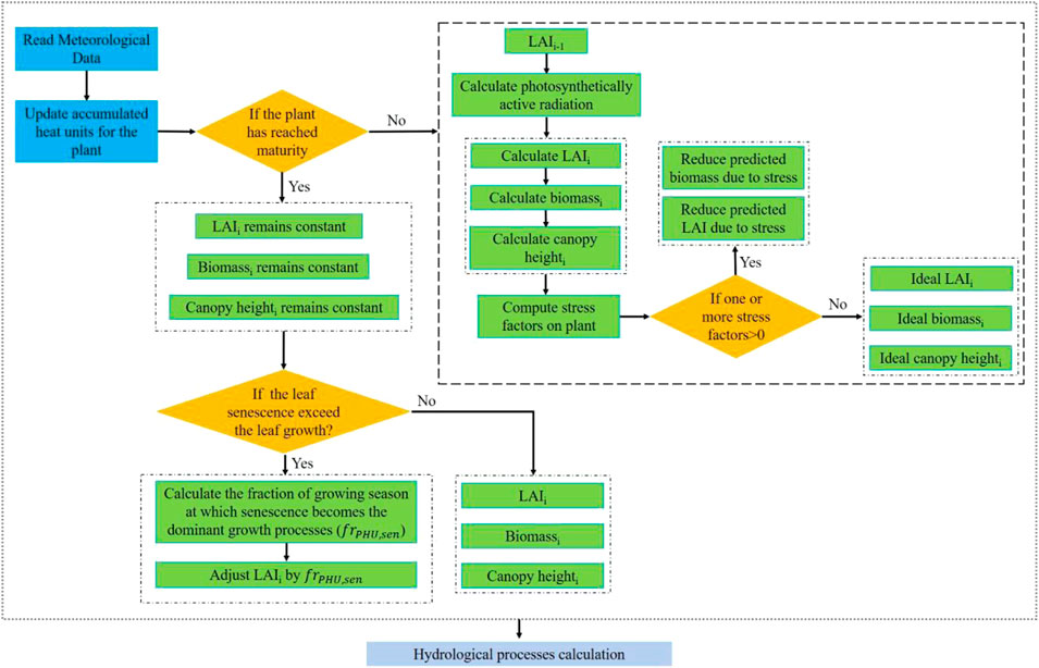
FIGURE 1. The plant growth module of the original Soil and Water Assessment Tool (SWAT) model.

2.2 Modifications to the Simulation of Vegetation Dynamics in SWAT

2.2.1 Derivation of the Land Use/Cover Classification

We derived land use/cover types using Landsat Operational Land Imager images of upper reaches of the Bayin River in 2018. Using a 1:50,000 topographic map as the datum and the Albers projection, images were geometrically corrected using a quadratic polynomial model. Interpretation keys of the images were established using land use maps and observed data for the same period, including 53 ground control points (to verify the accuracy). Next, we performed supervised human-machine classification and image interpretation using ArcGIS 10.7 (ESRI, Redlands, CA, United States) and the ENVI 5.6 image processing software (Harris Geospatial Solutions, Inc., Broomfield, CO, United States). Results were compared with land use maps of the study area for the corresponding period. On-site verification revealed that the qualitative accuracy of the data classification exceeded 93%. Compared with those of the existing land use maps of the study area, the kappa coefficients of the interpreted land use maps in this study exceeded 0.92. Main land cover types in the study area were grassland and barren land. We classified land use in this study as forest, grassland, water, residential, and barren land (Figure 2).

FIGURE 2

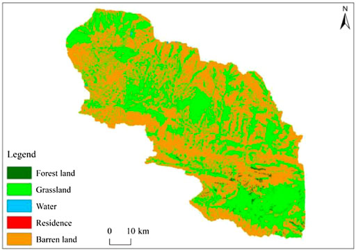
FIGURE 2. Land use/cover type in the study area.

2.2.2 Modifications to the Plant Growth Module

In the original SWAT model, plant growth module estimates plant growth and patterns based on the average vegetation density in each HRU, and LAI represents the growth status and coverage for one plant. Therefore, the LAI remains constant for one land cover type unless the hydrothermal and nutrient conditions differ between HRUs. To accurately derive the spatiotemporally heterogeneous LAI, we replaced the LAI calculation module and instead mapped the downscaled GLASS LAI to HRUs (Figure 3).

FIGURE 3

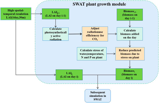
FIGURE 3. The modified plant growth module.

The spatial and temporal resolutions of the GLASS LAI product used in this study were 500 m and 8 days, respectively. However, the spatial resolution of land use/cover, soil, and the digital elevation model (DEM) used to derive HRUs was 30 m, and the time step of the SWAT model was 1 day. Therefore, the GLASS LAI product was downscaled to fit the SWAT model. The Enhanced Spatial and Temporal Adaptive Reflectance Fusion Model (ESTARFM) (Zhu et al., 2010) was used to produce fine-spatial-temporal-resolution LAI maps by fusing coarse-spatial-fine-temporal and fine-spatial-coarse-temporal remote sensing images. The ESTARFM contains two fusion methods: blend-then-index (BI) and index-then- blend (IB). BI inputs original images into the fusion model, blends them, and then calculates the index, whereas IB calculates the index based on original images, inputs the index maps to the fusion model, and then derives synthetic maps. Recently, IB has been shown to be generally more accurate than BI (Tian et al., 2013; Yan et al., 2018). Therefore, we used the IB approach to generate the synthetic LAI. The detailed fusion steps for the GLASS LAI and Landsat images were as follows:

(1) A regression model was established between the GLASS LAI and MOD13A1/MYD13A1 normalised difference vegetation index (NDVI).

(2) The Landsat-based NDVI was used with the regression model to obtain the Landsat-based LAI.

(3) The GLASS-based LAI was sampled to a 30 m resolution and the projection of the Landsat- and GLASS-based LAI data was uniformed.

(4) The Landsat- and GLASS-based LAI data were added to the ESTARFM model to obtain the 8-day LAI with a resolution of 30 m.

Spatially, one HRU may corresponding to mutiple LAI grids. Thus, to map the grid-based downscaled GLASS LAI to each HRU, we added the LAI of all the grids and calculated the average value for each corresponded HRU. The plant growth module was further modified to reflect the vegetation coverage for grassland. Moreover, we used the piecewise linear interpolation method to interpolate the 8-day GLASS LAI and derive the daily LAI to fit the time step of the SWAT model.

2.3 The Study Area

The Bayin River watershed is located between 96°30′ and 98°10′E and 37°02′ and 38°10′N in the northwest margin of the Qinghai-Tibetan Plateau, and is a typical inland river (or terminal lake) basin with a drainage area of approximately 10,000 km². The upper reach in Qilian Mountain has a drainage area of 6,499 km² and was selected as the study site (Figure 4). This area primarily generates the runoff for the entire basin (Jin and Jin, 2020). Its elevation ranges from 3,024 to 5,249 m, and the annual precipitation ranges from over 150 mm (in areas above 3,100 m) to 500 mm (at the summit). The dominant land cover types within the watershed is grassland with different vegetation covarage, and the main soil types are light frigid calcic soil and dark frigid calcic soil (Figure 4).

FIGURE 4

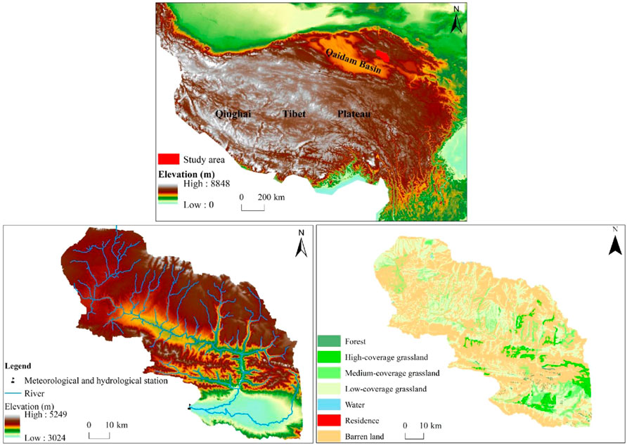
FIGURE 4. The study area.

2.4 The SWAT Model Setup

The following data sets for the study area were used to setup the SWAT model and evaluate its performance: 1) DEM with a spatial resolution of 30 m, 2) land use map with a spatial resolution of 30 m, 3) soil map with a spatial resolution of 30 m, 4) climatic data, including daily maximum and minimum air temperature and daily precipitation at Delingha Meteorological station (all climate data were obtained as daily averages), 5) the flow data at the outlet of the study watershed (Delingha Hydrological Station), 6) the sediment yield data at the outlet of the study watershed and 7) the Operational Simplified Surface Energy Balance model-simulated ET with a spatial resolution of 1 km (Lei et al., 2019). Apart from the ET data, all other datasets were provided by the National Tibetan Plateau/Third Pole Environment Data Centre of China (https://data.tpdc.ac.cn/en/).

The SWAT model was run at monthly intervals for various periods from 2013 to 2018: the warm-up period (2013), the calibration period (2014–2016), and the validation period (2017–2018). The model performance in fitting the observations was measured using three objective functions according to Moriasi et al. (2007): Nash–Sutcliffe efficiency (NSE) (Nash and Sutcliffe, 1970), percent bias (PBIAS), and coefficient of determination (R²). NSE measures the “goodness of fit” with a value ranging from 0 to 1 (indicating a perfect match). PBIAS measures the average tendency of the simulated values to be larger or smaller than the observed values, and is expressed as a percentage as follows: −10% to +10% represents a very good performance rating, and −25% to +25% represents a satisfactory performance rating. R² describes the proportion of variance in the measured data that is explained by the model. R² ranges from 0 to 1, with higher values indicating lower error variance. Values greater than 0.5 are typically considered acceptable (Nash and Sutcliffe, 1970; Moriasi et al., 2007; Jin et al., 2015). NSE, PBIAS, and R² were calculated as follows:

$NSE=1-\left[\frac{{{\displaystyle \sum }}_{i=1}^n{\left(V_i^{obs}-V_i^{sim}\right)}^2}{{{\displaystyle \sum }}_{i=1}^n{\left(V_i^{obs}-V^{mean}\right)}^2}\right](5)$

$PBIAS=\left[\frac{{{\displaystyle \sum }}_{i=1}^n\left(V_i^{obs}-V_i^{sim}\right)\times 100}{{{\displaystyle \sum }}_{i=1}^n{V}_i^{obs}}\right](6)$

$R^2=\frac{{\left[{{\displaystyle \sum }}_{i=1}^N\left(V_i^{sim}-{\overline{V}}^{sim}\right)\left(V_i^{obs}-{\overline{V}}_i^{obs}\right)\right]}^2}{{{\displaystyle \sum }}_{i=1}^N{\left(V_i^{sim}-{\overline{V}}^{sim}\right)}^2²{{\displaystyle \sum }}_{i=1}^N{\left(V_i^{obs}-{\overline{V}}^{obs}\right)}^2²}(7)$

3 Results

3.1 Sensitivity and Calibration of Parameters in SWAT

We built two SWAT models: the original SWAT model and the modified SWAT model based on the remotely sensed, spatiotemporally heterogenous and high-resolution LAI. Before calibrating and validating the models, we determined the most sensitive parameters—those were, key parameters and the degree of parameter precision required for calibration (Arnold et al., 2012; Jin et al., 2018). We used the monthly streamflow data from the Deingha Station (2014–2016) to conduct a sensitivity analysis of the original and modified SWAT models. Figure 5 shows results of the sensitivity analysis and lists the ten most sensitive parameters for streamflow simulation. The t-stat values (Figure 5) provide a measure of sensitivity (where larger absolute values indicate higher sensitivity) and the p-values indicate the significance of the sensitivity (where p-values close to zero indicate more significance). The first four parameters with highest sensitivity in the original (Figure 5A) and modified (Figure 5B) SWAT models were CN2 (initial SCS runoff curve number for moisture condition II), ALPHA_BF (base flow alpha factor), CH_K2 (effective hydraulic conductivity in the main channel alluvium), and SOL_BD (moist bulk density). The other sensitive parameters in the two models are listed Figure 5. See Arnold et al. (2011) for details regarding the parameters. These parameters were calibrated using the sequential uncertainty fitting version 2 algorithm in the SWAT-CUP software. After the calibration of streamflow-related parameters, four more sediment-related parameters were calibrated: LAT_SED (sediment concerntration in lateral and groundwater flow), USLE_P (USLE equation support practice factor), SPCON (Linear parameter for calculating the maximum amount of sediment that can be reentrained during chanel sediment routing) and SPEXP (exponent parameter for calculation sediment reentrained in channel sediment routing).

FIGURE 5

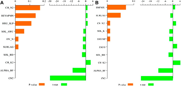
FIGURE 5. The sensitive parameters for the original (A) and modified (B) Soil and Water Assessment Tool (SWAT) models.

3.2 Remotely Sensed and SWAT-Simulated LAI

We downscaled the GLASS LAI to fit the basic calculation units of the SWAT model. Figures 6A,B shows a comparison of the downscaled and original GLASS LAI data. Pixels of the two LAI datasets had the same spatial distribution. Moreover, the downscaled LAI had a higher spatial resolution and provided more detailed spatial information. We calculated the monthly average LAI for the entire watershed based on the downscaled and original GLASS LAI datasets. The two datasets had the same patterns of seasonal variations, where the LAI was highest in July or August and lowest in January. While for the original SWAT model, the LAI reaches the peak value in June (Figure 6C). In almost every month, the remotely sensed LAI was noticeably higher than the original SWAT simulated value. The deviation of the downscaled and original GLASS LAI was −0.005 to 0.9 but 0.1–3.3 for the original SWAT simulated LAI and the two datasets; the lowest and the highest deviation were during the winter and during the summer months, respectively. The correlation of the monthly LAI derived from the two datasets was 0.9482 (Figure 6D). In summary, the downscaled remotely sensed LAI data were reliable. We mapped the grid-based downscaled GLASS (remotely sensed) LAI to each HRU. Figure 7 shows the remotely sensed and original SWAT-simulated long-term monthly average LAI mapped to the HRU level. For the entire watershed, the remotely sensed LAI was heterogeneous in each month. In contrast, in the original SWAT data, the simulated LAI was homogeneous in the same land use/cover types. In every month, the original SWAT simulated LAI was 0 for the barren land, slightly higher for the grassland, and highest for the sparsely distributed forest land (Figure 2).

FIGURE 6

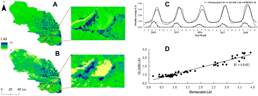
FIGURE 6. Comparisons of the downscaled leaf area index (LAI) and the original Global LAnd Surface Satellite (GLASS) LAI. (A) Spatial distribution of the downscaled LAI. (B) Spatial distribution of the original GLASS LAI. (C) Monthly variation of the downscaled LAI and GLASS LAI. (D) Correlation between the downscaled LAI and GLASS LAI.

FIGURE 7

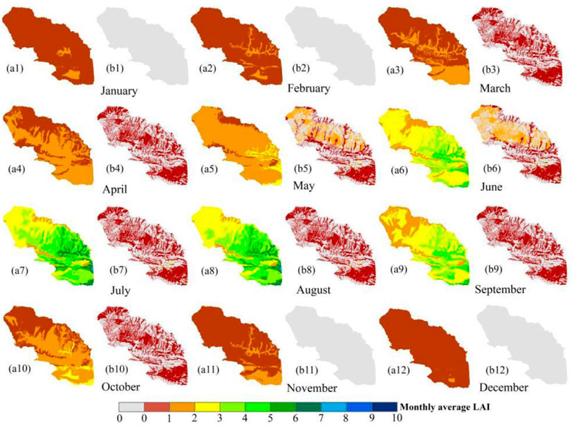
FIGURE 7. The remotely sensed (a1–a12) and Soil and Water Assessment Tool (SWAT)-simulated (b1–b12) long term (2014–2018) monthly average leaf area index (LAI) on hydrological response units (HRUs). The boundaries between the HRUs are not shown.

3.3 Simulations of the Streamflow

The performance of the original and modified SWAT models in simulating the monthly streamflow is shown in Figure 8 and Table 1. During the calibration and validation periods, the original SWAT model had the R² of over 0.87, the NSE over 0.85, and the PBIAS within 0–9%. For the modified SWAT, the R² was over 0.90, the NSE was over 0.89, and the PBIAS was within 0–4%. The performance of the modified SWAT to simulate the monthly streamflow was better than that of the original SWAT.

FIGURE 8

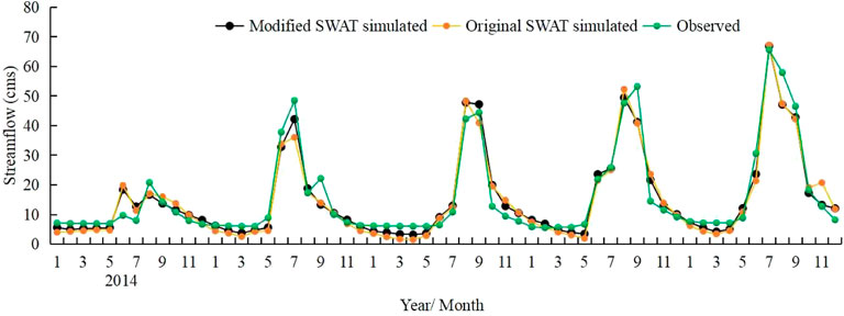
FIGURE 8. The monthly streamflow simulated by the original and modified Soil and Water Assessment Tool (SWAT) models compared to the that of observed streamflow.

TABLE 1

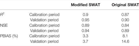
TABLE 1. The performance of the original and modified Soil and Water Assessment Tool (SWAT) models in simulating the monthly streamflow.

3.4 Simulations of the Sediment Yield

The performance of the original and modified SWAT models in simulating the monthly sediment yield is shown in Figure 9 and Table 2. During the calibration and validation periods, the original SWAT model had the R² of over 0.85, the NSE over 0.79, and the PBIAS within 15–28%. For the modified SWAT, the R² was over 0.87, the NSE was over 0.86, and the PBIAS was within −15 to 25%. The performance of the modified SWAT to simulate the monthly sediment yield was obviously better than that of the original SWAT.

FIGURE 9

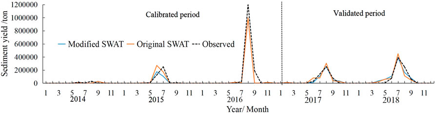
FIGURE 9. The monthly sediment yield simulated by the original and modified Soil and Water Assessment Tool (SWAT) models compared to the that of observed sediment yield.

TABLE 2

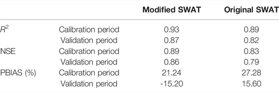
TABLE 2. The performance of the original and modified Soil and Water Assessment Tool (SWAT) models in simulating the monthly streamflow.

3.5 Simulations of the ET

The spatial resolution of the remotely sensed ET data was relatively high (1 km). Therefore, we analysed the performance of the original and modified SWAT models to simulate the monthly ET at subbasin level (Figure 10). The results demonstrated that in most subbasins, the R² and NSE values of the modified SWAT were higher than those of the original SWAT. Moreover, the absolute value of PBIAS was lower for the modified SWAT than for the original SWAT in most subbasins: During the calibration and validation periods, 82 and 83% of the subbasins for the modified SWAT had higher R² and NSE values than that for the original SWAT. For the modified and original SWAT, there were 62 and 55% of the subbasins had the PBIAS values in −25 to 25%, respectively, during both of the calibration and validation period. Therefore, the modified SWAT showed better performance than the original SWAT in simulating the monthly ET.

FIGURE 10

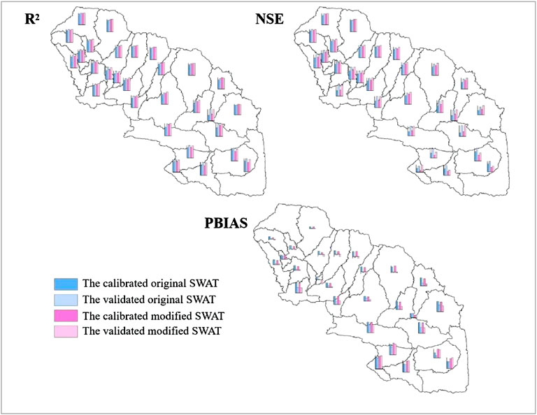
FIGURE 10. The performance of the original and modified Soil and Water Assessment Tool (SWAT) models in simulating the monthly evapotranspiration at the level of subbasins.

4 Discussion

The simulated LAI was homogeneous within a land use/cover type for the original SWAT, whereas the remotely sensed LAI was spatially heterogeneous and could better capture the vegetation coverage of the entire basin. The LAI calculated by the original SWAT was primarily affected by land use/cover types, water stress, temperature stress, nitrogen stress, and phosphorus stress (Arnold et al., 2012; Alemayehu et al., 2017). Only one meteorological station exist in the Bayin River Basin, and all of the vegetation is natural and without fertilisation. Therefore, in the original SWAT model, the spatial heterogeneity of LAI in Bayin River Basin was only determined by the land use/cover types (Figures 2, 7). The second-level classification of grassland (Figure 4) could reflect vegetation coverage (Jia et al., 2018). However, these land cover types are not included in the plant and land cover database of the SWAT (Arnold et al., 2012). Therefore, the original SWAT simulated LAI values were the same for one land cover type. This does not conform to the spatial heterogeneity of vegetation coverage especially within grassland (Figure 4) in Bayin River Basin (Wang et al., 2014; Yang et al., 2018). The downscaled remotely sensed LAI data in this study was reliable, because: 1) Most remotely sensed LAI products have gaps and missing values, and either underestimate or overestimate the LAI in many areas (Fensholt et al., 2004; Sun et al., 2014; Li et al., 2018), while the GLASS-based LAI used in this study was spatially and temporally continuous with no gaps and missing values and had high quality and accuracy in China (Zhao et al., 2013; Li et al., 2018; Xie et al., 2019). 2) The GLASS LAI was downscaled, and higher resolution LAI data would reduce the mismatch boundary of HRUs in SWAT models (Ma et al., 2019). The modified SWAT incorporated the downscaled remotely sensed LAI which could better reflect the spatiotemporal heterogeneity of the LAI and thus overcame the limitation of the original SWAT.

SWAT models are commonly calibrated and validated with streamflow and sediment yield data at the outlet of a watershed, which improves the reliability of the model simulations (Gassman et al., 2007; Jin et al., 2015; Yang et al., 2020). The improved LAI can improve the simulation results of the canopy interception loss, soil water content, runoff and further, the whole water budget in SWAT (Jaromir and Karsten, 2010; Zheng et al., 2018; Ma et al., 2019). Moreover, the erosion process would be improved because the SWAT model compute erosion caused by rainfall and runoff with the Modified Universal Soil Loss Equation (MULSE). In MUSLE, the average annual gross erosion is predicted as a function of runoff factor. Therefore, the modified SWAT that incorporated the high resolution LAI corresponded to a better estimation in streamflow and sediment yield. This study used high-resolution (1 km) remotely sensed ET data (SSEBop) to validate the original and modified SWAT models at the subbasin and HRU levels, because model performance should be analysed at a more detailed scale as well, especially when testing high-resolution input data (Alemayehu et al., 2017; Paul et al., 2020). SSEBop is also known to have a higher quality than several other datasets in grass covered surface (Herman et al., 2018; Dembélé et al., 2020). LAI is a key parameter that calculate the regional ET. Thus, the modified SWAT corresponded to a better estimation in ET. In summary, streamflow, sediment yield and ET which are the vegetation coverage-affected processes (Chen et al., 2006; Wang et al., 2021) were more accurate when using the remotely sensed high temporal and spatial resolution LAI. The spatial and temporal accuracy of the LAI was confirmed as being of crucial importance for SWAT predictions.

Coupling the SWAT model with the MODIS LAI product has been used for enhanced modelling of green vegetation dynamics (in tropical or subtropical areas) and crop patterns (in semi-arid areas), and may improve the applicability of SWAT in corresponding areas (Ma et al., 2019; Paul et al., 2020). The improvement of the SWAT in these studies was catalogued by the remotely sensed LAI, which could properly capture a more realistic plant phenology and patterns at a higher resolution. In this study, the remotely sensed LAI could capture the vegetation coverage of the grassland and barren land, which are the main land cover types for the whole study area. In addition, considerable areas of barren land have been converted to grassland under the impact of climate change and artificial vegetation restoration, and the vegetation coverage of grassland has increased in the Bayin River Basin (Jin et al., 2019). These changes can be elucidated in the LAI with high spatial and temporal resolution derived in this study.

The major limitations of this study are as follows: 1) There is only one meteorological station in the study area, which presented the only set of meteorological data. Although, two paraneters (PLAPS, precipiattion lapse rate; TLAPS, temperature lapse rate) were used to modify the precipitaion and temperature of the study area. This would still impose uncertainties in hydrological process modelling, especially in mountainous areas. 2) Piecewise linear interpolation was used to interpolate the 8 days and 30 m LAI data to the daily time interval. However, the LAI may not vary linearly, and this may cause some uncertainties.

5 Conclusion

Using remotely sensed LAI data with high spatiotemporal resolution, we modified the SWAT model to better simulate eco-hydrological processes in grassland basins with different vegetation coverages in the Bayin River Basin. Site-based streamflow, sediment yield data and remotely sensed ET data (at the subbasin and HRU levels) were used to estimate the performances of the original and modified SWAT models. We report two important findings. First, the simulated LAI was homogeneous within a land use/cover type for the original SWAT, whereas the remotely sensed LAI was spatially heterogeneous and could better capture the vegetation coverage of the entire basin. Second, the improved LAI may be used to simulate canopy interception loss, soil water content, and the water budget; therefore, the modified SWAT performed better than the original SWAT in simulating the hydrological processes.

Data Availability Statement

The original contributions presented in the study are included in the article/Supplementary Material, further inquiries can be directed to the corresponding author.

Author Contributions

Conceptualization, XJ; methodology, XJ; formal analysis, XJ; investigation, XJ; resources, YJ; data curation YJ and DF; writing—original draft preparation, XJ; writing—review and editing, YJ and XM; project administration, XJ; funding acquisition, XJ. All authors have read and agreed to the published version of the manuscript.

Funding

This research was supported by the National Natural Science Foundation of China, No. 42161020 and grants from the Natural Science Foundation of Qinghai Province, China, grant number 2021-ZJ-705.

Conflict of Interest

The authors declare that the research was conducted in the absence of any commercial or financial relationships that could be construed as a potential conflict of interest.

Publisher’s Note

All claims expressed in this article are solely those of the authors and do not necessarily represent those of their affiliated organizations, or those of the publisher, the editors and the reviewers. Any product that may be evaluated in this article, or claim that may be made by its manufacturer, is not guaranteed or endorsed by the publisher.

References

Alemayehu, T., van Griensven, A., Woldegiorgis, B. T., and Bauwens, W. (2017). An Improved SWAT Vegetation Growth Module and its Evaluation for Four Tropical Ecosystems. Hydrol. Earth Syst. Sci. 21 (9), 4449–4467. doi:10.5194/hess-21-4449-2017

CrossRef Full Text | Google Scholar

Arnold, J. G., Kiniry, J. R., Srinivasan, R., Williams, J. R., Haney, E. B., and Neitsch, S. L. (2011). Soil and Water Assessment Tool Input/Output File Documentation Version 2009. Texas Water Resources Institute.

Google Scholar

Arnold, J. G., Moriasi, D. N., Gassman, P. W., Abbaspour, K. C., White, M. J., Srinivasan, R., et al. (2012). SWAT: Model Use, Calibration, and Validation. Trans. ASABE 55 (4), 1491–1508. doi:10.13031/2013.42256

CrossRef Full Text | Google Scholar

Carlson, T. N., and Ripley, D. A. (1997). On the Relation between NDVI, Fractional Vegetation Cover, and Leaf Area Index. Remote Sens. Environ. 62 (3), 241–252. doi:10.1016/s0034-4257(97)00104-1

CrossRef Full Text | Google Scholar

Chen, S., Liu, Y., and Thomas, A. (2006). Climatic Change on the Tibetan Plateau: Potential Evapotranspiration Trends from 1961–2000. Clim. Change 76 (4), 291–319. doi:10.1007/s10584-006-9080-z

CrossRef Full Text | Google Scholar

Dembélé, M., Ceperley, N., Zwart, S. J., Salvadore, E., Mariethoz, G., and Schaefli, B. (2020). Potential of Satellite and Reanalysis Evaporation Datasets for Hydrological Modelling under Various Model Calibration Strategies. Adv. Water Resour. 143, 103667. doi:10.1016/j.advwatres.2020.103667

CrossRef Full Text | Google Scholar

Fang, H., Wei, S., and Liang, S. (2012). Validation of MODIS and CYCLOPES LAI Products Using Global Field Measurement Data. Remote Sens. Environ. 119, 43–54. doi:10.1016/j.rse.2011.12.006

CrossRef Full Text | Google Scholar

Feng, H., Zou, B., and Luo, J. (2017). Coverage-Dependent Amplifiers of Vegetation Change on Global Water Cycle Dynamics. J. Hydrol. 550, 220–229. doi:10.1016/j.jhydrol.2017.04.056

CrossRef Full Text | Google Scholar

Fensholt, R., Sandholt, I., and Rasmussen, M. S. (2004). Evaluation of MODIS LAI, fAPAR and the Relation between fAPAR and NDVI in a Semi-arid Environment Using In Situ Measurements. Remote Sens. Environ. 91 (3-4), 490–507. doi:10.1016/j.rse.2004.04.009

CrossRef Full Text | Google Scholar

Fu, L., Bo, T., Du, G., and Zheng, X. (2012). Modeling the Responses of Grassland Vegetation Coverage to Grazing Disturbance in an Alpine Meadow. Ecol. Model. 247, 221–232. doi:10.1016/j.ecolmodel.2012.08.027

CrossRef Full Text | Google Scholar

Gao, Q. Z., Li, Y., Wan, Y. F., Jiangcun, W-Z., Qin, X-B., and Wang, B-S. (2010). Significant Achievements in Protection and Restoration of Alpine Grassland Ecosystem in Northern Tibet, China. Restor. Ecol. 17 (3), 320–323. doi:10.1111/j.1526-100X.2009.00527.x

CrossRef Full Text | Google Scholar

Gassman, P. W., Reyes, M. R., Green, C. H., and Arnold, J. G. (2007). The Soil and Water Assessment Tool: Historical Development, Applications, and Future Research Directions. Trans. ASABE 50 (4), 1211–1250. doi:10.13031/2013.23637

CrossRef Full Text | Google Scholar

Guo, F., Nan, L., Chen, A. Q., and Gangcai, L. (2010). Influence of Vegetation Coverage on Surface Runoff and Soil Moisture in Rainy Season in Dry-Hot Valley. Agric. Sci. Technol.-Hunan 11 (4), 138–143. doi:10.16175/j.cnki.1009-4229.2010.04.003

CrossRef Full Text | Google Scholar

Herman, M. R., Nejadhashemi, A. P., Abouali, M., Hernandez-Suarez, J. S., Daneshvar, F., Zhang, Z., et al. (2018). Evaluating the Role of Evapotranspiration Remote Sensing Data in Improving Hydrological Modeling Predictability. J. Hydrol. 556, 39–49. doi:10.1016/j.jhydrol.2017.11.009

CrossRef Full Text | Google Scholar

Huang, S., Kumar, R., Flörke, M., Yang, T., Hundecha, Y., Kraft, P., et al. (2017). Evaluation of an Ensemble of Regional Hydrological Models in 12 Large-Scale River Basins Worldwide. Clim. Change 141 (3), 381–397. doi:10.1007/s10584-016-1841-8

CrossRef Full Text | Google Scholar

Jaromir, B., and Karsten, S. (2010). Retrieval of Leaf Area Index (LAI) and Soil Water Content (WC) Using Hyperspectral Remote Sensing under Controlled Glass House Conditions for Spring Barley and Sugar Beet. Remote Sens. 2 (7), 1702–1721. doi:10.3390/rs2071702

CrossRef Full Text | Google Scholar

Jia, N., Liu, J., Kuang, W., Xu, X., Zhang, S., Yan, C., et al. (2018). Spatiotemporal Patterns and Characteristics of Land-Use Change in China during 2010–2015. J. Geogr. Sci. 28 (5), 547–562. doi:10.1007/s11442-018-1490-0

CrossRef Full Text | Google Scholar

Jiang, H., Gong, J., Chen, X., and Liu, Y. (2019). Watershed-scale-based Forecast Method for Leaf Area Index Data Based on the Integration of Time Series MODIS Products and Meteorological Data. Environ. Earth Sci. 78 (15), 459. doi:10.1007/s12665-019-8477-8

CrossRef Full Text | Google Scholar

Jin, X., and Jin, Y. (2020). Calibration of a Distributed Hydrological Model in a Data-Scarce Basin Based on GLEAM Datasets. Water 12 (3), 897–910. doi:10.3390/w12030897

CrossRef Full Text | Google Scholar

Jin, X., Jin, Y., Yuan, D., and Mao, X. (2019). Effects of Land-Use Data Resolution on Hydrologic Modelling, a Case Study in the Upper Reach of the Heihe River, Northwest China. Ecol. Model. 404, 61–68. doi:10.1016/j.ecolmodel.2019.02.011

CrossRef Full Text | Google Scholar

Jin, X., He, C., Zhang, L., and Zhang, B. (2018). A Modified Groundwater Module in SWAT for Improved Streamflow Simulation in a Large, Arid Endorheic River Watershed in Northwest China. Chin. Geogr. Sci. 28 (1), 47–60. doi:10.1007/s11769-018-0931-0

CrossRef Full Text | Google Scholar

Jin, X., Zhang, L., Gu, J., Zhao, C., Tian, J., and He, C. (2015). Modelling the Impacts of Spatial Heterogeneity in Soil Hydraulic Properties on Hydrological Process in the Upper Reach of the Heihe River in the Qilian Mountains, Northwest China. Hydrol. Process. 29 (15), 3318–3327. doi:10.1002/hyp.10437

CrossRef Full Text | Google Scholar

Karlsson, I. B., Sonnenborg, T. O., Refsgaard, J. C., Trolle, D., Børgesen, C. D., Olesen, J. E., et al. (2016). Combined Effects of Climate Models, Hydrological Model Structures and Land Use Scenarios on Hydrological Impacts of Climate Change. J. Hydrol. 535, 301–317. doi:10.1016/j.jhydrol.2016.01.069

CrossRef Full Text | Google Scholar

Lai, G., Luo, J., Li, Q., Qiu, L., Pan, R., Zeng, X., et al. (2020). Modification and Validation of the SWAT Model Based on Multi-Plant Growth Mode, a Case Study of the Meijiang River Basin, China. J. Hydrol. 585, 124778. doi:10.1016/j.jhydrol.2020.124778

CrossRef Full Text | Google Scholar

Lei, J., Senay, G. B., Velpuri, N. M., and Stefanie, K. (2019). Evaluating the Temperature Difference Parameter in the SSEBop Model with Satellite-Observed Land Surface Temperature Data. Remote Sens. 11 (16), 1947–1962. doi:10.3390/rs11161947

CrossRef Full Text | Google Scholar

Li, X., Lu, H., Yu, L., and Yang, K. (2018). Comparison of the Spatial Characteristics of Four Remotely Sensed Leaf Area Index Products over China: Direct Validation and Relative Uncertainties. Remote Sens. 10 (2), 148–173. doi:10.3390/rs10010148

CrossRef Full Text | Google Scholar

Ma, T., Duan, Z., Li, R., and Song, X. (2019). Enhancing SWAT with Remotely Sensed LAI for Improved Modelling of Ecohydrological Process in Subtropics. J. Hydrol. 570, 802–815. doi:10.1016/j.jhydrol.2019.01.024

CrossRef Full Text | Google Scholar

Moriasi, D. N., Arnold, J. G., Liew, M., Bingner, R. L., Harmel, R. D., and Veith, T. L. (2007). Model Evaluation Guidelines for Systematic Quantification of Accuracy in Watershed Simulations. Trans. ASABE 50 (3), 885–900. doi:10.13031/2013.23153

CrossRef Full Text | Google Scholar

Nash, J. E., and Sutcliffe, J. V. (1970). River Flow Forecasting through Conceptual Models Part I - A Discussion of Principles. J. Hydrol. 10 (3), 282–290. doi:10.1016/0022-1694(70)90255-6

CrossRef Full Text | Google Scholar

Neitsch, S. L., Arnold, J. G., Kiniry, J. R., and Williams, J. R. (2011). Soil and Water Assessment Tool Theoretical Documentation Version 2009. Temple: Texas Water Resources Institute.

Google Scholar

Pang, S., Wang, X., Melching, C. S., and Feger, K.-H. (2020). Development and Testing of a Modified SWAT Model Based on Slope Condition and Precipitation Intensity. J. Hydrol. 588, 125098. doi:10.1016/j.jhydrol.2020.125098

CrossRef Full Text | Google Scholar

Parajuli, P. B., Nelson, N. O., Frees, L. D., and Mankin, K. R. (2010). Comparison of AnnAGNPS and SWAT Model Simulation Results in USDA-CEAP Agricultural Watersheds in South-Central Kansas. Hydrol. Process. 23 (5), 748–763. doi:10.1002/hyp.7174

CrossRef Full Text | Google Scholar

Paul, M., Rajib, A., Negahban-Azar, M., Shirmohammadi, A., and Srivastava, P. (2021). Improved Agricultural Water Management in Data-Scarce Semi-Arid Watersheds: Value of Integrating Remotely Sensed Leaf Area Index in Hydrological Modeling. Sci. Total Environ. 791, 148177. doi:10.1016/j.scitotenv.2021.148177

PubMed Abstract | CrossRef Full Text | Google Scholar

Strauch, M., and Volk, M. (2013). SWAT Plant Growth Modification for Improved Modeling of Perennial Vegetation in the Tropics. Ecol. Model. 269, 98–112. doi:10.1016/j.ecolmodel.2013.08.013

CrossRef Full Text | Google Scholar

Sun, C., Liu, L., Guan, L., Quanjun, J., and Dailiang, P. (2014). Validation and Error Analysis of the MODIS LAI Product in Xilinhot Grassland. J. Remote Sens. 18 (3), 518–536. doi:10.11834/jrs.20143097

CrossRef Full Text | Google Scholar

Sun, J., Hou, G., Liu, M., Fu, G., Zhan, T., Zhou, H., et al. (2019). Effects of Climatic and Grazing Changes on Desertification of Alpine Grasslands, Northern Tibet. Ecol. Indic. 107, 105647. doi:10.1016/j.ecolind.2019.105647

CrossRef Full Text | Google Scholar

Tian, F., Wang, Y., Fensholt, R., Wang, K., Zhang, L., and Huang, Y. (2013). Mapping and Evaluation of NDVI Trends from Synthetic Time Series Obtained by Blending Landsat and MODIS Data Around a Coalfield on the Loess Plateau. Remote Sens. 5 (9), 4255–4279. doi:10.3390/rs5094255

CrossRef Full Text | Google Scholar

Wang, Q., Liu, R., Men, C., Guo, L., and Miao, Y. (2019). Temporal-Spatial Analysis of Water Environmental Capacity Based on the Couple of SWAT Model and Differential Evolution Algorithm. J. Hydrol. 569, 155–166. doi:10.1016/j.jhydrol.2018.12.003

CrossRef Full Text | Google Scholar

Wang, X., Luo, Y., Sun, L., and Shafeeque, M. (2021). Different Climate Factors Contributing for Runoff Increases in the High Glacierized Tributaries of Tarim River Basin, China. J. Hydrol. Regional Stud. 36, 100845. doi:10.1016/j.ejrh.2021.100845

CrossRef Full Text | Google Scholar

Wang, X., Ma, M., Song, Y., Tan, J., and Wang, H. (2014). Coupling of a Biogeochemical Model with a Simultaneous Heat and Water Model and its Evaluation at an Alpine Meadow Site. Environ. Earth Sci. 72 (10), 4085–4096. doi:10.1007/s12665-014-3300-z

CrossRef Full Text | Google Scholar

Xiao, Z., Liang, S., Wang, J., Xiang, Y., Zhao, X., and Song, J. (2016). Long-Time-Series Global Land Surface Satellite Leaf Area Index Product Derived from MODIS and AVHRR Surface Reflectance. IEEE Trans. Geoscience Remote Sens. 54 (9), 5301–5318. doi:10.1109/tgrs.2016.2560522

CrossRef Full Text | Google Scholar

Xie, X., Li, A., Jin, H., Tan, J., Wang, C., Lei, G., et al. (2019). Assessment of Five Satellite-Derived LAI Datasets for GPP Estimations through Ecosystem Models. Sci. Total Environ. 690 (10), 1120–1130. doi:10.1016/j.scitotenv.2019.06.516

PubMed Abstract | CrossRef Full Text | Google Scholar

Yan, Y., Liu, X., Wang, F., Li, X., Ou, J., Wen, Y., et al. (2018). Assessing the Impacts of Urban Sprawl on Net Primary Productivity Using Fusion of Landsat and MODIS Data. Sci. Total Environ. 613-614, 1417–1429. doi:10.1016/j.scitotenv.2017.09.139

PubMed Abstract | CrossRef Full Text | Google Scholar

Yang, D., Shao, W., Yeh, J. F., Yang, H., Kanae, S., and Oki, T. (2009). Impact of Vegetation Coverage on Regional Water Balance in the Nonhumid Regions of China. Water Resour. Res. 45 (7), 507–519. doi:10.1029/2008wr006948

CrossRef Full Text | Google Scholar

Yang, K., Wang, C., and Li, S. (2018). Improved Simulation of Frozen‐thawing Process in Land Surface Model (CLM4. 5). J. Geophys. Res. Atmos. 123 (23), 13238–13258. doi:10.1029/2017jd028260

CrossRef Full Text | Google Scholar

Yang, L., Feng, Q., Yin, Z., Deo, R. C., Wen, X., Si, J., et al. (2020). Regional Hydrology Heterogeneity and the Response to Climate and Land Surface Changes in Arid Alpine Basin, Northwest China. Catena 187, 104345. doi:10.1016/j.catena.2019.104345

CrossRef Full Text | Google Scholar

Zhang, X., Du, X., and Zhu, Z. (2020). Effects of Precipitation and Temperature on Precipitation Use Efficiency of Alpine Grassland in Northern Tibet, China. Sci. Rep. 10 (1), 20309. doi:10.1038/s41598-020-77208-6

PubMed Abstract | CrossRef Full Text | Google Scholar

Zhao, X., Liang, S., Liu, S., Yuan, W., Xiao, Z., Liu, Q., et al. (2013). The Global Land Surface Satellite (GLASS) Remote Sensing Data Processing System and Products. Remote Sens. 5 (5), 2436–2450. doi:10.3390/rs5052436

CrossRef Full Text | Google Scholar

Zheng, G., and Moskal, L. M. (2009). Retrieving Leaf Area Index (LAI) Using Remote Sensing: Theories, Methods and Sensors. Sensors 9 (4), 2719–2745. doi:10.3390/s90402719

PubMed Abstract | CrossRef Full Text | Google Scholar

Zheng, J., Fan, J., Zhang, F., Yan, S., and Xiang, Y. (2018). Rainfall Partitioning into Throughfall, Stemflow and Interception Loss by Maize Canopy on the Semi-arid Loess Plateau of China. Agric. Water Manag. 195, 25–36. doi:10.1016/j.agwat.2017.09.013

CrossRef Full Text | Google Scholar

Zhu, W., Jia, S., Lü, A., and Yan, T. (2012). Analyzing and Modeling the Coverage of Vegetation in the Qaidam Basin of China: The Role of Spatial Autocorrelation. J. Geogr. Sci. 22 (2), 346–358. doi:10.1007/s11442-012-0931-4

CrossRef Full Text | Google Scholar

Zhu, X., Chen, J., Gao, F., Chen, X., and Masek, J. G. (2010). An Enhanced Spatial and Temporal Adaptive Reflectance Fusion Model for Complex Heterogeneous Regions. Remote Sens. Environ. 114 (11), 2610–2623. doi:10.1016/j.rse.2010.05.032

CrossRef Full Text | Google Scholar