Blue carbon ecosystem monitoring using remote sensing reveals wetland restoration pathways

Lanceman, Dana; Sadat-Noori, Mahmood; Gaston, Troy; Drummond, Christopher; Glamore, William

doi:10.3389/fenvs.2022.924221

ORIGINAL RESEARCH article

Front. Environ. Sci., 03 November 2022

Sec. Conservation and Restoration Ecology

Volume 10 - 2022 | https://doi.org/10.3389/fenvs.2022.924221

Blue carbon ecosystem monitoring using remote sensing reveals wetland restoration pathways

Dana Lanceman^1,2*

Mahmood Sadat-Noori¹

Troy Gaston³

Christopher Drummond¹

William Glamore¹

¹Water Research Laboratory, School of Civil & Environmental Engineering, UNSW Sydney, Kensington, NSW, Australia
²School of Biological, Earth and Environmental Sciences, UNSW Sydney, Kensington, NSW, Australia
³School of Environmental and Life Sciences, University of Newcastle, Ourimbah, NSW, Australia

In an era of climate and biodiversity crises, ecosystem rehabilitation is critical to the ongoing wellbeing of humans and the environment. Coastal ecosystem rehabilitation is particularly important, as these ecosystems sequester large quantities of carbon (known in marine ecosystems as “blue carbon”) thereby mitigating climate change effects while also providing ecosystem services and biodiversity benefits. The recent formal accreditation of blue carbon services is producing a proliferation of rehabilitation projects, which must be monitored and quantified over time and space to assess on-ground outcomes. Consequently, remote sensing techniques such as drone surveys, and machine learning techniques such as image classification, are increasingly being employed to monitor wetlands. However, few projects, if any, have tracked blue carbon restoration across temporal and spatial scales at an accuracy that could be used to adequately map species establishment with low-cost methods. This study presents an open-source, user-friendly workflow, using object-based image classification and a random forest classifier in Google Earth Engine, to accurately classify 4 years of multispectral and photogrammetrically derived digital elevation model drone data at a saltmarsh rehabilitation site on the east coast of Australia (Hunter River estuary, NSW). High classification accuracies were achieved, with >90% accuracy at 0.1 m resolution. At the study site, saltmarsh colonised most suitable areas, increasing by 142% and resulting in 56 tonnes of carbon sequestered, within a 4-year period, providing insight into blue carbon regeneration trajectories. Saltmarsh growth patterns were species-specific, influenced by species’ reproductive and dispersal strategies. Our findings suggested that biotic factors and interactions were important in influencing species’ distributions and succession trajectories. This work can help improve the efficiency and effectiveness of restoration planning and monitoring at coastal wetlands and similar ecosystems worldwide, with the potential to apply this approach to other types of remote sensing imagery and to calculate other rehabilitation co-benefits. Importantly, the method can be used to calculate blue carbon habitat creation following tidal restoration of coastal wetlands.

1 Introduction

Wetlands are ecosystems that are permanently, seasonally or intermittently inundated with water and exist in the transition zone between terrestrial and aquatic ecosystems (Junk et al., 2014). Wetlands support high levels of biodiversity, providing habitats, food and breeding grounds for many taxa, including fish and waterbirds (Saintilan and Rogers, 2013). Wetlands also provide many important services to humans, including flood mitigation (Narayan et al., 2017), water filtration (Aziz and Van Cappellen, 2021) and carbon sequestration (Burden et al., 2019). However, wetlands have been particularly negatively impacted by anthropogenic activities and are rapidly declining (Mckee et al., 2012; Saintilan and Rogers, 2013; Boon et al., 2015). Due to these declines, there is an urgent need to conserve and restore wetlands, and all ecosystems, as recognised by the United Nations, who declared 2021–2030 as the “Decade of Ecosystem Restoration” (Waltham et al., 2020).

“Blue carbon” is the term used to describe carbon sequestered and stored by coastal marine ecosystems, including coastal wetlands. Blue carbon ecosystem rehabilitation is an increasingly recognised approach towards mitigating climate change, while also providing other biodiversity and ecosystem service benefits (McLeod et al., 2011). This is because coastal wetlands, including mangroves, saltmarshes and seagrasses, sequester more carbon per area (McLeod et al., 2011) and can accumulate and store carbon in soils for longer periods (Howard et al., 2017) than terrestrial ecosystems. Rehabilitating coastal wetlands is an effective approach to increasing blue carbon sequestration, by restoring or creating new areas to accumulate and store carbon in vegetation and soils (Howard et al., 2017). On-ground rehabilitation of blue carbon habitats is becoming increasingly economically viable, with landowners able to secure accredited carbon credits by rehabilitating natural ecosystems in many countries (Warren-Rhodes et al., 2011; Um, 2021). Even at coastal rehabilitation sites not explicitly targeted for carbon sequestration, blue carbon is increasingly quantified as a rehabilitation co-benefit. Methods for verifying blue carbon habitats are currently in early stages of development and include Verra’s blue carbon conservation methodology (Verra, 2020) and the blue carbon method under Australia’s Emission Reduction Fund (Commonwealth of Australia, 2022). These methodologies require accurate input data on spatial and temporal changes in blue carbon ecosystem areas over time, which are also necessary for growing our understanding of restoration trajectories and informing developments in restoration approaches. As such, there is a growing need for robust and low-cost workflows to track blue carbon ecosystems over various spatial and temporal domains.

Remote sensing techniques are one potential option to quantify blue carbon ecosystem areas, which can then be converted to blue carbon volumes using known or measured carbon sequestration rates for each species/ecosystem (e.g., Lovelock et al., 2013). Remote sensing allows data to be collected objectively and on larger spatial and temporal scales than via ground-based surveys, especially across intertidal wetlands, which are often difficult to access (Pham et al., 2019). In particular, unmanned aerial vehicles (UAVs–henceforth referred to as drones) are relatively inexpensive, flexible and convenient platforms that are widely accessible and can collect optical, thermal, multispectral and/or elevation data. Drones have the capacity to collect very high resolution data (up to 0.55 cm; Dronova et al., 2021), potentially enabling high accuracy and precision in coastal wetland monitoring. While studies frequently monitor on unitemporal or bitemporal scales (e.g., Kelly et al., 2011; Meng et al., 2017), drones allow flexibility in monitoring frequency, and there is scope for exploring the benefits of multitemporal surveys for rehabilitation monitoring (Ridge and Johnston, 2020). The use of drone imagery to quantify blue carbon ecosystem rehabilitation is a good starting point to explore the applicability of aerial monitoring techniques and to understand how high-accuracy methods might be adapted for lower resolution satellite imagery.

For remote sensing data to be useful for blue carbon quantification and other purposes, images must be accurately classified, or used to build maps showing the distribution of different land cover types. In the blue carbon context, this classification should ideally be undertaken on a species level, to understand vegetative biodiversity and species-specific trends, and because different wetland vegetation species have different life histories and carbon sequestration capabilities (Lovelock et al., 2013) and can support different faunal species (Laegdsgaard, 2006). The two main approaches used to classify remote sensing data are pixel-based methods, which classify each pixel individually, and object-based methods, which classify clusters of adjacent pixels with similar characteristics (Chapple and Dronova, 2017; Pham et al., 2019; Proença et al., 2019). Object-based methods are considered more accurate for classifying very high resolution data (Pham et al., 2019; Tmušić et al., 2020). Object-based image analysis (OBIA) or geographic OBIA (GEOBIA) groups pixels into segments and then categorises these segments into classes, based on their characteristics (Dronova, 2015; Kucharczyk et al., 2020). OBIA uses spectral, contextual (position of objects relative to one another), textural (spectral range within objects) and geographic (shape and size of objects) “features” or attributes of segments for classification, with different studies using different combinations of these features for classification (Kucharczyk et al., 2020).

There are many software applications that support OBIA (Kucharczyk et al., 2020), with the most popular option being the dedicated software eCognition (Dronova, 2015; Ma et al., 2017). While eCognition has a user interface and is feature-rich, it is a commercial software and thereby less accessible. Open-source software options for OBIA have been developed, including GRASS GIS (Grippa et al., 2017), Orfeo Toolbox (Grizonnet et al., 2017), InterIMAGE (De Costa et al., 2010), RSGISLib (Shepherd et al., 2019), SPRING (Câmara et al., 1996) and Google Earth Engine (Tassi and Vizzari, 2020). However, while there have been numerous publications exploring different algorithms for classification, including for OBIA (e.g. Hossain and Chen, 2019; Pham et al., 2019; Wen and Hughes 2020), few papers have focused on developing workflows for these diverse software options. Some of these options, such as Orfeo Toolbox, also have limited support communities online, making classification difficult when unknown errors are encountered. Within the wetlands context, open-source options only account for a few previously published studies in the literature (Dronova, 2015), with even fewer open-source multitemporal (but see Myers et al., 2018) or restoration studies. Hence, to encourage accurate and accessible wetland monitoring in a time when wetland rehabilitation is rapidly increasing, there is a need for object-based wetland classification studies with clear open-source workflows.

This study aims to demonstrate an approach for accurately tracking blue carbon at a rehabilitation site over time, while addressing several methodological gaps in remote sensing and image classification approaches to coastal wetland monitoring. To this aim, first we demonstrate an effective, open-source and user-friendly method for remote sensing monitoring of blue carbon restoration sites. Second, we produce accurate classifications on a species-level. Third, as image resolution is known to be important for accurate detection of fine-scale details (Dronova et al., 2021), we investigate what resolution is necessary for accurate saltmarsh rehabilitation monitoring. Fourth, in assessing the trajectory of blue carbon growth at a rehabilitation site (as detailed in Sadat-Noori et al., 2021), we develop an understanding of temporal, spatial, environmental and biological aspects of blue carbon restoration. This involves generating and analysing a series of accurate classified maps and tracking saltmarsh recovery over a 4-year period (January 2017 to December 2020) at an intertidal site, including an assessment of:

1) Overall area of rehabilitated blue carbon habitat (i.e., saltmarsh).

2) Spatial patterns in saltmarsh growth (i.e., patch metrics).

3) Temporal trends in saltmarsh growth.

4) Differences in growth patterns/trends between saltmarsh species.

5) Influence of elevation on saltmarsh regrowth.

These findings will help inform future restoration planning, particularly in the southern hemisphere, where there is a lack of wetland remote sensing studies (Pham et al., 2019).

2 Methods

2.1 Study site

The present study focuses on Fish Fry Flat (∼20 ha), part of a Ramsar-listed coastal wetland on Kooragang Island, Hunter Wetlands National Park, NSW, Australia (Figure 1). Kooragang Island is located within the Hunter River estuary, has a temperate climate (Bureau of Meteorology, 2022a), with 1,100 mm average annual rainfall (Bureau of Meteorology, 2022b), and facilitates multiple mangrove and saltmarsh ecosystems. Since the 1970s, at least 67% of Kooragang Island’s saltmarsh has been lost, mainly due to anthropogenic hydrological changes allowing greater tidal flows to the region, sea level rise and subsequent mangrove encroachment (Rogers et al., 2013). In response to greater tidal flows since the 1990s, the saltmarsh and mudflat ecosystems of the study site (Fish Fry Flat) have been increasingly outcompeted by grey mangroves (Avicennia marina), causing a loss of important shorebird habitat (Williams et al., 2000). In 2016, a saltmarsh rehabilitation program was initiated, with the primary aim of restoring shorebird habitat. This involved using Smart (flood) Gate systems to reinstate a tidal flushing regime designed to encourage saltmarsh growth (see Sadat-Noori et al., 2021; Rankin et al., 2022). This rehabilitation process, starting with a bare site and facilitating natural saltmarsh recruitment and regeneration (i.e. no planting) over time, provided a useful opportunity to explore remote-sensing monitoring techniques for blue-carbon rehabilitation. In brief, the rehabilitation process involved applying a tidal replicate method to control tidal flows into the estuary, creating an inundation pattern that favours saltmarsh ecosystems (see Sadat-Noori et al., 2021). Changes in the mean ground surface elevations of saltmarsh were anticipated following these deliberate changes to the wetland’s tidal regime, and adaptive management strategies were undertaken to reduce saltmarsh loss at high elevations (Sadat-Noori et al., 2021).

FIGURE 1

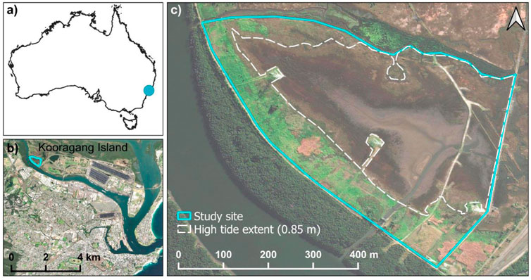
FIGURE 1. Study site extent with respect to: (A) Australia, (B) Kooragang Island and (C) Fish Fry Flat, also showing high tide extent. Imagery source: ESRI.

2.2 Data collection

2.2.1 Drone surveys

Since tidal restoration began at Fish Fry Flat, drone flights have been regularly conducted to monitor the site (Table 1). High density elevation data and high resolution RGB aerial imagery were collected using an eBee Real-Time Kinematic (RTK) fixed wing drone or a DJI Phantom four RTK multirotor, while high-resolution multispectral (green, red, red edge and near infrared) data were collected using an eBee Ag fixed wing drone equipped with a Parrot Sequoia multispectral sensor (Table 1). Drone flights were programmed to fly autonomously at a flight height of 120 m with 80% forward lap and sidelap. To improve geometric accuracy, a minimum of six Ground Control Points (GCPs) were evenly distributed around the study site for each survey flight. Flights were timed to maximise uniformity of cloud cover and minimise atmospheric effects on image quality. The adjustable floodgates were set to ensure minimum water levels onsite during the surveys. Ground sampling distances (GSDs–distances between pixels) were approximately 3 cm for RTK surveys and approximately 12 cm for multispectral surveys.

TABLE 1

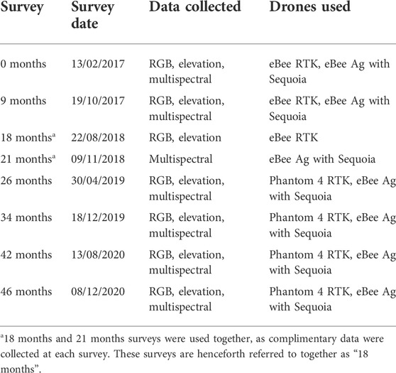
TABLE 1. Summary of data collected on drone flights at Fish Fry Flat rehabilitation site between 2017 and 2020. RTK = Real Time Kinematic and refers to the ability of the drone to collect location and elevation data.

2.2.2 On-ground vegetation survey

Vegetation surveys were conducted around the same date as each drone survey, sampling saltmarsh vegetation at varying ground surface elevations (see Rankin et al., 2022). These vegetation data were used to visualise major saltmarsh species in the drone imagery and guide the selection of training and validation points for classification. Vegetation sampling identified three major saltmarsh species in the study area; Sporobolus virginicus (sand couch), Sarcocornia quinqueflora (glasswort) and Suaeda australis (seablite), however, other saltmarsh and invasive weed species are known to exist on site (Rankin et al., 2022).

2.3 Pre-processing

Initial pre-processing of the RGB and multispectral aerial imagery was completed in Pix4D Mapper software package (Pix4D SA, 2021) to produce georeferenced orthomosaic images (stitched together spectral images) and 3D digital surface models (DSMs–elevation maps). Images were reprojected from WGS84 to a local projected coordinate system, GDA 1994 MGA Zone 56. Ground Control Point (GCP) locations were input into the software and the rayCloud editor used to match GCPs with at least 20–30 images per GCP. The XYZ georeferencing accuracy of each dataset was validated to a root mean square error (RMSE) of <0.02 m when compared to the GCP positions. Point clouds were generated at half image size with a minimum of three matching images per point and an “optimal” point density. For RGB/RTK data, orthomosaics were created and DSMs generated using noise filtering, surface smoothing and the Inverse Distance Weighting method. For multispectral drone imagery, radiometric processing and “Camera, Sun Irradiance and Sun Angle” calibrations were done using input reflectance panel photographs for each spectral band. Radiometric calibration images were corrupt for one survey date (9 months) and these data were processed using “no correction”. Reflectance panel photographs with moderate lighting were used where possible. Green, Red, Red Edge, Near Infrared and Normalised Difference Vegetation Index (NDVI) reflectance maps were generated.

To ensure consistent georeferencing among images, multispectral reflectance maps were georeferenced to their RGB counterparts in QGIS version 3.8.3 (QGIS Development Team, 2021) using four to five manually selected link points per image (Supplementary Table S1). Artificial structures (e.g. cement foundation blocks, pipelines) with distinct corners were used as reference points to increase precision. A first-order polynomial or affine transformation was applied. It was aimed to keep the RMSE under 0.1 m, however, this was not possible for one image, where obvious artificial structures were not well captured (Supplementary Table S1). Images were rectified using cubic convolution, which has been shown to produce the highest-quality results for aerial imagery (Rizeei and Pradhan, 2019). Subsequently, all images were clipped to the study area extent (Figure 1C). Multispectral images were then resampled to the higher resolution DSM cell size, to preserve elevation data detail. Band ranges for multispectral bands and the DSM were standardised to a range of 0–255 (8 bits), to ensure an equal weighting of all bands, as required for many classifiers, including random forest (Immitzer et al., 2016; De Luca et al., 2019). Finally, all multispectral rasters and the DSM were merged into multiband rasters for each survey date, to use as inputs for classification. An overview of pre-processing procedures is provided in Supplementary Figure S1.

2.4 Image classification

Image classification was performed on multiband rasters with five spectral bands (Green, Red, Red Edge, Near Infrared and NDVI) and one elevation band (DSM).

2.4.1 Object-based image analysis

Object-based image analysis (OBIA) was used for classification, as it is increasingly recognised to produce superior results to pixel-based techniques for classifying wetlands (Tmušić et al., 2020). OBIA involves first segmenting images, based on their spectral and/or elevation values, into “objects” of an appropriate size for the landscape element/s of interest (in our case, saltmarsh plants) (Hossain and Chen, 2019). Then, “features” or attributes (such as mean elevation) relating to these image objects are derived for each object (Kucharczyk et al., 2020). Training data are generated for the classes of interest, and are used with the segmented image and feature data to train a machine-learning classifier (Kucharczyk et al., 2020).

2.4.2 Google Earth Engine

Google Earth Engine was used for image classification because it is an open-source, cloud-based platform that uses a programming language (JavaScript) (Gorelick et al., 2017) and supports OBIA. Google Earth Engine is a computationally efficient platform for image classification, as data are stored as rasters for the entire classification process, greatly reducing computation times, compared with classification processes that polygonise images (Tassi and Vizzari, 2020). Google Earth Engine is usually used for analysing open-source remote sensing data that are available within its data inventory, such as Landsat and Sentinel-2 imagery (Gorelick et al., 2017), but can also be used for analysing user-specific data, such as the drone data used in this study.

2.4.3 Segmentation

The first step of object-based classification is segmentation, where the input multiband image is segmented into meaningfully sized image objects (Hossain and Chen, 2019). In Google Earth Engine, segmentation was performed using a Simple Non-Iterative Clustering (SNIC) function. In SNIC, objects were grown iteratively from “seeds” that were distributed evenly throughout the image. Neighbouring pixels around each seed with similar image attributes for each band were grouped together to form objects, so that each generated object represented a single land-cover type. The most accurate results were achieved with parameters seed = 5, compactness = 1, connectivity = 8 and neighbourhoodSize = 10. The seed parameter represents the number of pixels between objects’ starting locations; a small number was chosen so that object edges, and hence small saltmarsh clumps, could be accurately captured. Compactness refers to the squareness of objects; a small number was used so that objects were less square. Connectivity refers to directions of growth for objects (adjacent vs. adjacent and diagonal growth); we allowed both adjacent and diagonal growth. Neighbourhood size refers to the radius of pixels used when merging objects from adjacent tiles, which are used to increase computation speed; we used the default value of double the seed value.

2.4.4 Feature extraction

Object attributes, known as “features”, were then extracted. There are hundreds of possible features that can be derived in this process (e.g. Hladik and Alber, 2014; Wan et al., 2014; Dronova, 2015; Husson et al., 2016; Chapple and Dronova, 2017; Husson et al., 2017; Murfitt et al., 2017; Chabot et al., 2018; Kucharczyk et al., 2020). These features fall into several categories: elevation (relating to elevation data), spectral (relating to spectral bands), textural (relating to the range and distribution of pixels within an object), contextual (relating to the proximity of objects to important features in the landscape) and geometric (relating to the shape and size of objects) (Kucharczyk et al., 2020). For the present study, we synthesised the range of features employed in previous studies and considered the tools available for feature extraction in Google Earth Engine to derive the set of features listed in Table 2. Due to the functionality of Google Earth Engine’s tools, some of these features needed to be calculated in neighbourhoods across the entire image, and later averaged during segmentation. These included Grey-Level Co-occurrence Matrix features (correlation, inverse difference moment, contrast and angular second moment) and entropy, which are all measures of texture. Other features were calculated for each object after segmentation: mean, standard deviation, kurtosis (steepness of peak in frequency distribution curve), skewness (asymmetry of frequency distribution curve), area and perimeter.

TABLE 2

TABLE 2. Features used for classification and examples of their use in previous wetland classification studies.

2.4.5 Classes of interest

Three saltmarsh classes were selected for classification, representing the three most common native saltmarsh species at our study site: Sporobolus virginicus (co-dominant), Sarcocornia quinqueflora (co-dominant) and Suaeda australis (non-dominant). Five environmental classes were also selected: “grass”, which also included other non-saltmarsh vegetation (including weeds), “mud”, which included all bare soil/clay/mud, “dead vegetation”, “water” and “road”. For the first post-rehabilitation dataset (9 months), Sarcocornia quinqueflora was broken up into two classes, representing young and old saltmarsh clumps, as the original model had difficulty recognising small, young saltmarsh clumps. Suaeda australis was not classified in either of the first two datasets, as it was not present at 0 months (area = 0 ha) and made up a very small area, insufficient for classification, at 9 months. For the 42 months dataset, “algae” was included as an additional class, as it was prevalent during this time period and easily misclassified as saltmarsh.

2.4.6 Generation of training and validation datasets

Ground-truth data from field-based vegetation surveys (Sadat-Noori et al., 2021) were used to identify the appearance of saltmarsh species on the drone imagery. In QGIS (QGIS Development Team, 2021), 100 points were then digitally selected within each class in every orthomosaic, ensuring these points represented the full variability within the class, were evenly spaced throughout the image (i.e., there were no large areas without training points) and were independent of one another (i.e., not close together) (Dronova, 2015). An equal number of points was selected for each class to reduce underestimation and overestimation of small and large classes, respectively (Kucharczyk et al., 2020). High quality training/validation data were especially important for early datasets, where saltmarsh clumps were harder to distinguish, and in some cases training/validation data were iteratively revised to produce more accurate classifications. For each orthomosaic, 50% of the chosen points were randomly selected for training and 50% for validation, as recommended in a review of OBIA accuracy assessments (Ye et al., 2018), and as a balance between time efficiency and classification accuracy. While it has been suggested that larger training/validation datasets might improve classification accuracy (Kucharczyk et al., 2020), we found limited improvements in accuracy when testing with 100, 200 or 300 data points on a sample dataset.

2.4.7 Classification

A random forest classifier was used for image classification, as random forest has consistently produced highly accurate results in previous wetland classification studies (Pham et al., 2019). Random forest parameters were set at numberOfTrees = 500 and minLeafPopulation = 1, as these parameter values produced the most accurate results. The classification was run at several resolutions to evaluate the impact of resolution on classification accuracy: 0.1 m (equivalent to the lowest resolution of our input data), 0.5 m, 1 m and 2 m resolutions. The GINI importance (relative importance for classification; Pasquarella et al., 2018) of each feature (Table 2) in each classification was evaluated, and model training and validation accuracy calculated by comparing landcover classes in classified images to manually selected validation points (Section 2.4.6), as often done in image classification studies (e.g. Pande-Chhetri et al., 2017; Ventura et al., 2018), using confusion matrixes. Confusion matrixes estimate producer’s accuracy (percent of manually selected points in each class that were correctly classified), user’s accuracy (percent of classified points in each class that are truly that class) and overall accuracy (percent of correctly classified points across all classes). Then, each classification was iteratively run with the 1–56 most important feature/s to determine the smallest number of features that produced the most accurate (highest overall validation accuracy) classification for each dataset/resolution combination. The “seed” argument within the random forest classifier was varied to ensure reproducibility, and was found not to impact classification results. Classified maps were exported using the optimal number of features for each dataset at the 0.1 m resolution.

2.5 Data analysis

All data analysis was performed in RStudio Version 1.2.5 (patch metrics) and 1.4.1106 (all other analysis) (RStudio Team, 2021), using the 0.1 m resolution data.

To test for differences in the GINI importance of different features and bands for classification, a factorial ANOVA was computed using the importance values for each feature/band combination for each dataset (n = 7), after checking normality and equal variance assumptions. There was a significant interaction between feature and band, so a post hoc Tukey’s test was run to test for differences between feature/band combinations, and to determine which features/bands were most important for classification models.

To explore saltmarsh growth patterns, ecologically-relevant patch metrics (as identified by previous studies: Gonzalez et al., 2019; Kelly et al., 2011) were calculated for each classified image using the package landscapemetrics version 1.5.4 (Hesselbarth et al., 2019). Selected class-level patch metrics were patch area, class area, core area, number of patches, cohesion, Euclidean nearest-neighbour distance, clumpiness, contiguity and shape, while landscape-level metrics were contagion, Shannon’s diversity and Shannon’s evenness (Table 3). These metrics related to research questions (Table 3). Temporal trends in patch metrics were investigated with Kendall rank correlations, using the package Kendall version 2.2 (McLeod, 2011), and changes in area were quantified.

TABLE 3

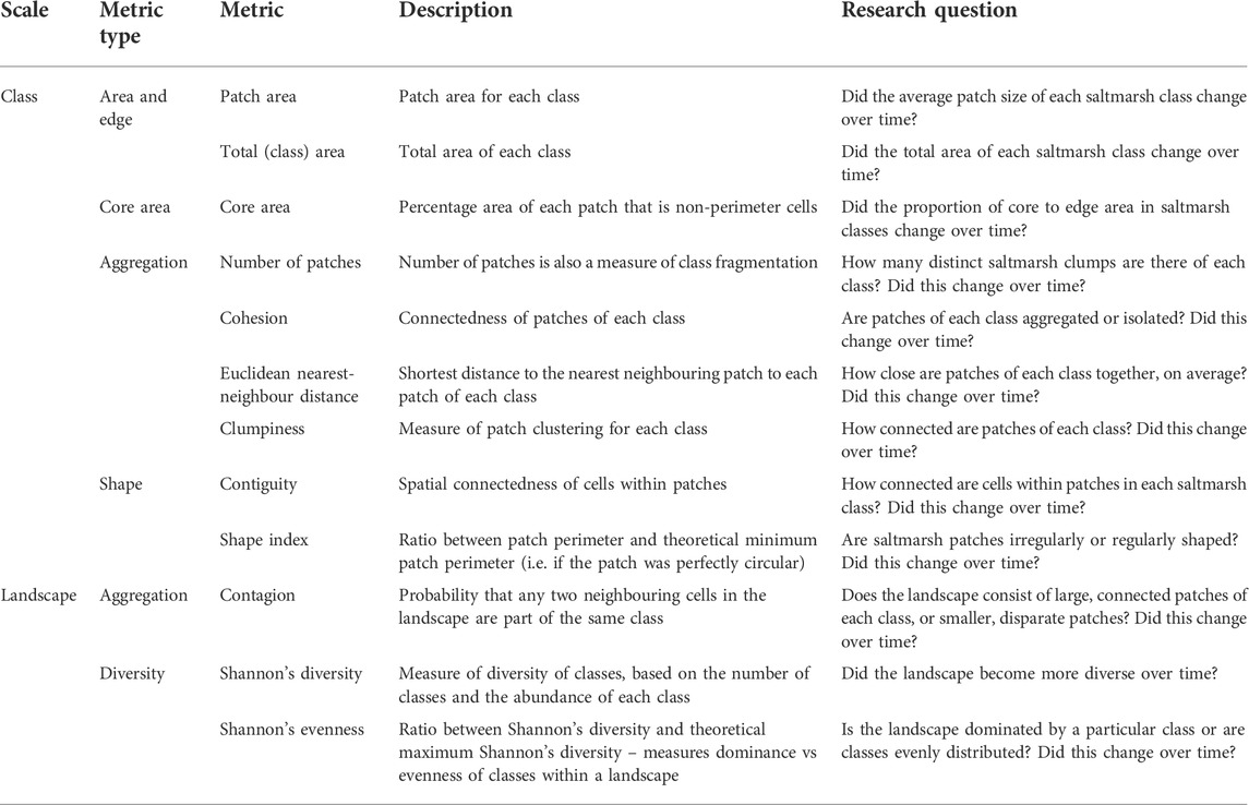
TABLE 3. Class- and landscape-level patch metrics calculated from classified images, and relevant research questions.

To understand how saltmarsh growth and loss have contributed to net area changes, spatial changes in Sporobolus virginicus and Sarcocornia quinqueflora between the 0 months and 46 months datasets, and between each pair of successive datasets, were explored in QGIS (QGIS Development Team, 2021). Areas of saltmarsh growth (non-saltmarsh to saltmarsh transition), loss (saltmarsh to non-saltmarsh transition) and species transition were calculated. Changes in Suaeda australis were not calculated because of issues with this species’ classification accuracy.

Changes in the mean ground surface elevation of saltmarsh species were also investigated. The initial DSM (bare ground—0 months) was intersected with the classified images to determine the mean ground surface elevation of each saltmarsh class in each dataset, and the mean elevation where saltmarsh growth, loss and transitions occurred over time. Then, temporal trends in mean elevation for each species were investigated using Kendall rank correlations (McLeod, 2011).

2.6 Blue carbon calculations

The BlueCAM method was recently developed by the Australian Government under the Emissions Reductions Fund as a method for calculating carbon sequestration by coastal ecosystems using input data related to climate, elevation, hydrology, wetland type, area and time (Australian Government Clean Energy Regulator, 2022; Commonwealth of Australia, 2022). This method was used to estimate blue carbon volumes sequestered by rehabilitated saltmarsh based on blue carbon ecosystem areas. The climate region was “tropical humid” and relevant parameters included a 25-year permanence period and a 1.6 m tidal regime, identified using water level monitoring data collected on site over the 4-year monitoring period (see Sadat-Noori et al., 2021). The average elevation of rehabilitated saltmarsh was calculated as an additional parameter. We only calculated carbon sequestered and did not account for carbon emissions, which would have been generated from vehicle travel, smart gate creation, etc., and would need to be considered for full carbon budgeting. The model was run for the study period to calculate carbon abated during this time. The model was also used to project carbon volumes after 10, 20, 30, 40 and 50 years post-rehabilitation, assuming saltmarsh areas remained stable over these timeframes.

The entire processing workflow, showing the major steps involved from aerial imagery capture to blue carbon calculations, is summarised in Supplementary Figure S2. All code used for classification and analysis is available in the Data Accessibility section (Lanceman, 2022).

3 Results

The image classification produced seven classified maps at 0.1 m resolution (Figure 2).

FIGURE 2

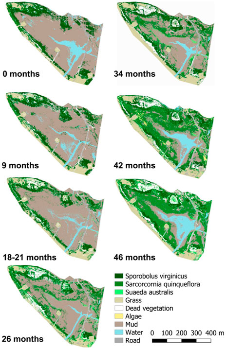
FIGURE 2. Classified drone images (0.1 m resolution) indicating land cover changes post rehabilitation. Note that water cover is variable between images because the wetland is a dynamic system that experiences natural and synthetically mimicked (via automated floodgates; Sadat-Noori et al., 2021) variations in tidal inundation over multiple timescales.

3.1 Classification success

The number of features required to produce the most accurate classification varied between datasets and resolutions (between 3 and 28; Supplementary Table S2). In all datasets, classification accuracy initially increased rapidly when including more features, reaching an approximate plateau with less than 10 features, and often decreasing slightly with additional features. In a factorial ANOVA modelling the importance of feature/band combinations, there was a significant interaction between feature and band (F = 6.3, SS = 81,605, MS = 2040, df = 40, p <0.001). A Tukey’s test revealed that the “mean” values of each band were significantly more important (all p <0.05) than all other features in the model (n = 50, Supplementary Figure S3). Mean elevation was the most important feature in the model, with significantly greater importance (all p < 0.001) than all other features (n = 55, Supplementary Figure S3).

For these most accurate classifications, training overall accuracy was consistently very high (0.997–1) across datasets for 0.1 m and 0.5 m resolutions and high (0.943–0.998) for 1 m and 2 m resolutions (Supplementary Table S3). Validation overall accuracy was very high (>∼0.9) for 0.1 m resolution, high (>0.8) for 0.5 m and 1 m resolutions, and moderate (0.685–0.786) for 2 m resolution (Supplementary Table S3). Validation producer’s accuracy and user’s accuracy similarly decreased with coarsening resolution, and were relatively consistent across datasets (Supplementary Figure S4, Supplementary Figure S5). For the 0.1 m resolution classified images, user’s and producer’s accuracies were always above 75%, and usually above 85%, for all saltmarsh species (Supplementary Figure S4, Supplementary Figure S5). Resolution had a greater impact on the producer’s and user’s accuracy of saltmarsh species than most other classes (Supplementary Figure S4, Supplementary Figure S5).

3.2 Growth patterns

Saltmarsh area significantly increased by 6.39 ha (142%) at the site over the 4-year period after rehabilitation (Kendall rank correlation, tau = 0.905, p = 0.007, Figure 3). The most substantial change in saltmarsh area occurred in Sarcocornia quinqueflora, which significantly increased by 5.75 ha (595%) over the 4-year monitoring period (tau = 0.905, p = 0.007, Figure 3). Suaeda australis also significantly increased by 1.60 ha (tau = 0.867, p = 0.02, Figure 3). Sporobolus virginicus experienced a net decline in area (0.96 ha or 27%) over time, however this change was non-significant (tau = -0.238, p = 0.55, Figure 3).

FIGURE 3

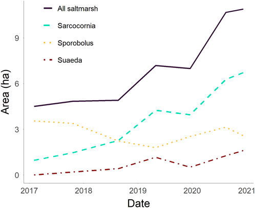
FIGURE 3. Change in saltmarsh area over time post rehabilitation at the study site. Areas were calculated using 0.1 m resolution classified images with > 75% user's and producer's accuracy for each species Supplementary Figure S4, Supplementary Figure S5).

Spatial analysis of saltmarsh trends revealed that over time, an area of 2.18 ha of Sporobolus virginicus was lost (including transitions to non-saltmarsh and to Sarcocornia quinqueflora), mainly around the outer parts of its distribution, while 1.28 ha grew elsewhere, mainly in inner areas (Figure 4; Table 4). Simultaneously, 0.85 ha of Sarcocornia quinqueflora was lost, mostly in outer areas, while 6.62 ha grew more centrally (Figure 4; Table 4).

FIGURE 4

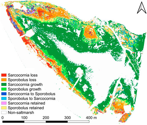
FIGURE 4. Spatial changes in Sporobolus virginicus and Sarcocornia quinqueflora over the study period (46 months): loss (saltmarsh to non-saltmarsh), growth (non-saltmarsh to saltmarsh), transitions between species and retention (saltmarsh retained over time).

TABLE 4

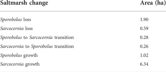
TABLE 4. Changes in Sporobolus virginicus and Sarcocornia quinqueflora over the study period (46 months). “Loss” refers to locations where saltmarsh was converted into a non-saltmarsh land cover, while “transition” refers to changes between saltmarsh species, and “growth” refers to where non-saltmarsh land cover was converted into saltmarsh.

Patch metrics analyses highlighted differences in growth patterns between species and over time (Figure 5). Sarcocornia quinqueflora experienced the most notable changes in patch metrics over time, significantly increasing in mean patch area (Kendall rank correlation, tau = 0.81, p = 0.02), mean core area index (Kendall rank correlation, tau = 0.71, p = 0.04), cohesion (Kendall rank correlation, tau = 0.91, p = 0.007) and mean contiguity (Kendall rank correlation, tau = 0.71, p = 0.04) over time (Figure 5). Sarcocornia quinqueflora also exhibited a (non-significant) hump-shaped time series for number of patches, and an inverse hump-shaped time series for clumpiness (Figure 5). There were no significant trends in any metric for either of the other species over time, and no notable trends in Euclidean nearest neighbour distance or shape index. Suaeda australis exhibited distinctive growth patterns, with much smaller patch sizes and lower values for cohesion and clumpiness (Figure 5) than the other species. Sporobolus virginicus had relatively consistent values for all patch metrics, notably having consistently very high values for cohesion and clumpiness (Figure 5). In terms of landscape-level patch metrics, there was a significant increasing trend in Shannon’s diversity over time (Kendall rank correlation, tau = 0.81, p = 0.02), while trends in contagion and Shannon’s evenness were non-significant (Supplementary Figure S6).

FIGURE 5

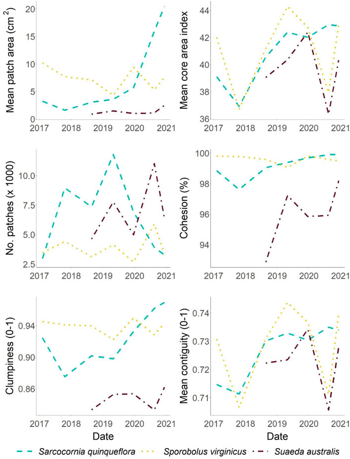
FIGURE 5. Class-level patch metrics: mean patch area, mean core area index (percentage of each patch that is non-edge cells), number of patches, cohesion (connectedness of patches of the same class), clumpiness (proportion of adjacent patches that are the same class) and mean contiguity (connectedness of cells within patches) for three saltmarsh classes (Sporobolus virginicus, Sarcocornia quinqueflora and Suaeda australis). There are missing data for Suaeda australis because it was not classified in the first two dataset.

There was a significant negative trend in the mean ground surface elevation that Sarcocornia quinqueflora grew at over time (Kendall rank correlation, tau = -1, p = 0.003), changing from 0.9 m pre-rehabilitation to 0.5 m after 46 months (Supplemementary Figure S7). There were no trends in elevation for either of the other species (Supplementary Figure S7). Sarcocornia quinqueflora growth mainly occurred at low elevations (∼0.5 m), while loss/transitions occurred at high elevations (∼0.9 m) (Supplementary Figure S8). Sporobolus virginicus growth occurred at middle elevations (∼0.7 m), while loss occurred at higher elevations (∼0.8 m) and transitions to Sarcocornia quinqueflora occurred at lower elevations (∼0.6 m) (Supplementary Figure S8).

3.3 Blue carbon quantification

When all input data were entered into BlueCAM (Section 2.6), the blue carbon accounting model estimated that the additional 6.39 ha of saltmarsh that grew during the study period resulted in 31.9 tonnes carbon being sequestered in above-ground biomass and 43 tonnes in soil. This makes a total of 56.2 tonnes of carbon abated, given a 25-year permanence period. Carbon abatement was projected to increase over time at a slower, linear rate, with ∼129 tonnes of carbon projected to be abated after 10 years and ∼464 tonnes after 50 years.

4 Discussion

This study developed a highly accurate image classification workflow for monitoring blue carbon restoration over time at a species level. By classifying a 4-year time series of drone images at a rehabilitation site, we identified spatial and temporal growth trends, and differences in growth patterns between saltmarsh species, which will be useful for informing future rehabilitation strategies. Our workflow was almost entirely open-source, and thereby very accessible. The workflow could be made entirely open-source by using freely available software for drone photogrammetry processing such as those recommended by Myburgh et al. (2021), although this may reduce accuracy.

4.1 Classification success

The classifications were highly accurate at 0.1 m (90–94%) and 0.5 m (85–94%) resolutions, greater than accuracy levels commonly reported in wetland classification studies (Dronova, 2015; Ye et al., 2018). In reviews of 209 and 61 OBIA studies, respectively, Ye et al. (2018) and Dronova (2015) both found an average overall accuracy level of 85%, lower than our accuracies. Given we maintained accuracies at > 80% at 1 m pixel resolution, and that there are now at least 15 satellite sensors that produce images at resolutions of 0.3–1 m (Satellite Imaging Corporation, 2022), there is substantial potential worldwide to undertake accurate high-resolution image classification using a workflow similar to ours with commercial satellite imagery. This would allow wetland monitoring on much larger scales than possible with drones or ground-based surveys. However, only two current satellite sensors (Satellogic and SkySat-C) provide multispectral imagery with ≤1 m resolution (Satellite Imaging Corporation, 2022), and imagery from all commercial satellites is expensive to acquire. There is currently no freely available satellite imagery at these ultra-high resolutions, posing a barrier for areas with limited funding. In addition, satellites do not generally capture elevation data, which we found to be the most important band for producing accurate classifications. Since we found that accuracies were strengthened with multiple image bands and decreased substantially at 2 m resolution, we caution undertaking species-level wetland classifications, particularly at rehabilitation sites with small vegetation clumps like saltmarsh, using satellite imagery with resolutions >1 m. Therefore, if funding allows, commercial satellites could permit large-scale, high-frequency monitoring with acceptable accuracies. If not, drones remain a good option for more accessible and affordable monitoring at smaller scales. More research is needed to better understand the differences in wetland restoration classification between drones and other high-resolution remote-sensing options, especially those that generate different types of spectral and elevation data.

Classification accuracy was dependent on which object features were used for classification. Band means were the most important features for classification, but it was almost always necessary to also include other types of features for optimal accuracy (Supplementary Table S2). There was no consistency in which additional features were needed to improve accuracy, and previous studies have also not agreed on to which features are most important for classification (Chapple and Dronova, 2017; Espriella et al., 2020). Therefore, for effective classification, we suggest calculating a range of feature types (as shown in this study), and then selecting the optimal set of features for each dataset. Computation of many features using a cloud-based approach like Google Earth Engine can be achieved in seconds, hence there are few disadvantages in starting with excessive features. Given that mean elevation was the most important feature for image classification, our study has provided evidence that using elevation and multispectral data together improves classification accuracy, as suggested by previous studies (e.g., Husson et al., 2017; Doughty and Cavanaugh, 2019; Digiacomo et al., 2020), especially for photogrammetrically-derived DSMs (Pinton et al., 2021). This makes sense, because boundaries between mudflats, saltmarsh species and terrestrial vegetation are strongly driven by tidal inundation depths (Clarke and Hannon, 1970). Therefore, it is suggested that future studies also consider these data types together.

We were able to accurately classify saltmarsh vegetation to a species level. Classifications were more effective, and training/validation data required less revisions, for species with larger clumps and for later datasets (i.e., after clumps had grown larger). Although our models produced high user’s and producer’s accuracy for all saltmarsh species, visual observation of classified images revealed that Suaeda australis had been consistently overestimated across datasets and resolutions, with these errors likely also explaining inconsistencies in elevation for this species (Supplementary Figure S7). This may reflect a potential minimum threshold in the area or density of classes needed for accurate classification. The inconsistency between reported and observed accuracy is likely due to the small size of Suaeda australis clumps, making them less likely to intersect with a validation point. More work should be done to improve classification accuracy of minor components of the landscape, such as using a hierarchical classification that first breaks the landscape into broader groups and then classifies within these groups (Husson et al., 2016). Such technique development may also allow classification of less common wetland species, which were not considered for classification in this study.

4.2 Spatial and temporal trends in saltmarsh growth

The use of multitemporal data allowed exploration of temporal trends in rehabilitation, revealing insights about natural saltmarsh colonisation patterns at a site with tidal conditions artificially optimised to promote saltmarsh growth and limited ongoing management (see Sadat-Noori et al., 2021; Rankin et al., 2022). Saltmarsh growth rates were relatively linear over time, but increased after 18 months (Figure 3). The initial lag in regeneration may reflect the time period required for saltmarsh establishment and existing organic matter decomposition (e.g., 15% degradation of fibrous mangrove roots over 9 months in south-east Australia; Van der Valk and Attiwill, 1984), as the major saltmarsh species, Sarcocornia quinqueflora, struggles to establish where there is existing above- or below-ground biomass (Genders, 1996). The time lag could also reflect seed availability (Erfanzadeh et al., 2009), initial lack of mutualistic fauna (Derksen-Hooijberg et al., 2017), time required for saltmarsh clumps to mutualistically support one another (Silliman et al., 2015), or climatic differences between years or seasons. For example, increased rainfall and/or inundation can promote saltmarsh growth by decreasing salinity stress (Breen et al., 1977; Laegdsgaard, 2006; Green et al., 2009), while high salinity levels inhibit Sarcocornia quinqueflora germination (Partridge and Wilson, 1987). Given southeast Australia experienced a severe drought during the first 3 years post-rehabilitation (Bureau of Meteorology, 2020), climatic stressors likely contributed to lagged growth rates and saltmarsh transitions to dead vegetation and weeds (Figure 2, Figure 3). At our site, and at other rehabilitation sites involving altered hydrology, the initial lag could also be related to simultaneous saltmarsh loss and growth (Figure 4) as species shift in elevation (Supplementary Figure S7) due to the deliberately altered tidal regime, also likely contributing to the net decline in Sporobolus virginicus over time (Figure 4; Table 4). Time lags in regeneration should be anticipated in other rehabilitation studies, and monitoring of relevant environmental, biological and climate factors would be useful to identify which factors are driving growth rates at each specific site.

Saltmarsh growth would be expected to plateau once all suitable bare areas have been colonised, with an upper growth limit controlled by elevation/inundation and pasture grass competition (Streever and Genders, 1997). In our study, most bare areas were colonised by saltmarsh after 4 years, with landscape diversity also increasing during this time (Supplementary Figure S6), aligning with timeframes of other nearby rehabilitation sites (e.g., ∼5 years; Glamore et al., 2021; Laegdsgaard, 2006). This indicates that saltmarsh rehabilitation via natural regeneration can occur relatively quickly, providing insight into trajectories of blue carbon restoration at saltmarsh rehabilitation sites in south-east Australia. While substantial growth in vegetation suggests a successful trajectory towards rehabilitation, it is likely the site will continue to evolve in both cover and biodiversity into the future, and continued monitoring, as well as comparison with control and reference sites, would allow for the calculation of rehabilitation timeframes and validation of carbon accumulation rates. Knowledge of blue carbon accumulation rates will help in predicting blue carbon volumes at sites over various timescales, with the next challenge in blue carbon accounting being predicting changes in the price of carbon into the future.

Classifying saltmarsh to the species level allowed identification of differences in growth patterns, which reflect species’ morphology and reproductive strategies. The three saltmarsh species classified in this study are competitors (Zedler et al., 1995) that occupy similar tidal heights (Hickey and Bruce, 2010), and their distribution at a rehabilitation site is largely dependent on the relative suitability of conditions and reproductive strategy of each species. The marsh ecotype of Sporobolus virginicus reproduces almost exclusively via rhizome production by extending underground stems (Blits and Gallagher, 1991), mainly expanding from existing vegetation (Figure 4), reflecting its consistently high patch metrics values for cohesion, clumpiness and patch area (Figure 5). Conversely, Sarcocornia quinqueflora and Suaeda australis regenerate via seeding (Green et al., 2009), and can create new saltmarsh clumps across the landscape (Figure 2). This patchiness is reflected in Suaeda australis’s consistently low values for cohesion, clumpiness and patch area, and Sarcocornia quinqueflora’s hump-shaped trends for number of patches and clumpiness, as it produced many new clumps that eventually merged into larger patches (Figure 5). Sarcocornia quinqueflora is known to reproduce and disperse rapidly in favourable conditions (Laegdsgaard, 2002) by producing large quantities of buoyant, tidally-dispersed, desiccation-resistant seeds (Nelson, 1994). Conversely, Sporobolus virginicus is known to expand more slowly (Laegdsgaard, 2002), reflecting our observed differences in growth rates between species (Figure 3; Table 4). Our study demonstrates that investigating multitemporal trends in patch metrics can provide useful insights into species’ growth patterns and reproductive strategies. The results also suggest that leaving a site to regenerate naturally, with appropriate tidal inundation patterns, will favour faster-growing species that are better dispersers.

In this study, Sarcocornia quinqueflora was the most dominant species, with increasing dominance over time, as its seeding dispersal and rapid reproduction allowed it to outcompete other species and limit their realised niches (biologically restricted distributions), similar to species interactions observed in previous saltmarsh rehabilitation studies (Erfanzadeh et al., 2009; Sullivan et al., 2018), including at sites in Australia with similar species assemblages (Green et al., 2009). Depending on co-benefits targeted at rehabilitation sites, single-species dominance may be acceptable, for example if saltmarsh area and growth speed are primary goals. However, for sites aiming for biodiversity, a more balanced distribution of saltmarsh species may be desirable, to support a greater range of faunal species (Laegdsgaard, 2006). To facilitate this, a mixed rehabilitation approach could be employed based on target species’ ecology. For example, growth of slower-growing species like Sporobolus virginicus could be encouraged via planting, while allowing natural regeneration of more competitive species (Green et al., 2009; Winning and MacFarlane, 2010). However, deliberate encouragement of slower-growing species may not be necessary, as it is possible that a more balanced distribution of species could naturally evolve over time. For example, studies have suggested that succession may occur in regenerating saltmarsh sites, where Sarcocornia quinqueflora is gradually outcompeted by Sporobolus virginicus (Adam, 1990; Zedler et al., 1995). Longer-term monitoring is required to assess the ongoing evolution of the site’s biodiversity.

4.3 Blue carbon and co-benefits

The 56.2 tonnes of carbon (Section 3.3) abated by rehabilitated saltmarsh during the study period are equivalent to the amount of carbon produced by 12 passenger vehicles over a year (United States Environmental Protection Agency, 2018). If the saltmarsh rehabilitation area remained stable at 6.4 ha, it is projected to abate ∼8.4 tonnes (1.3 tonnes per hectare) carbon per year, equivalent to emissions from two cars each year. This is similar to the trajectory and rate of carbon accumulation measured or modelled in previous saltmarsh rehabilitation studies (Burden et al., 2019; Santini et al., 2019). Over larger spatial scales of rehabilitation, much more substantial quantities of carbon could be abated, contributing to climate change mitigation strategies. In addition, as carbon accounting methods are further developed, species differences in carbon sequestration (Lovelock et al., 2013) may be able to be accounted for, leading to more accurate carbon calculations.

There is great potential for remote sensing technologies to monitor rehabilitation co-benefits beyond blue carbon. For example, remote sensing has also been used at coastal and wetland sites to quantify waterbird usage (Francis et al., 2020), count people (i.e., measure tourism) (Provost et al., 2019) and investigate hydrological dynamics (Wu et al., 2019), with potential implications for quantifying hydrological ecosystem services such as flood mitigation. A combined remote sensing approach that quantified a broader range of rehabilitation co-benefits would allow more aspects of blue carbon ecosystems to be valued, providing further economic incentives for their rehabilitation.

5 Conclusion

By developing a user-friendly workflow for classifying drone imagery, this study has provided insight into blue carbon restoration and monitoring procedures. We achieved very high classification accuracy using multispectral and photogrammetric elevation data, object-based methods and a random-forest classifier in the Google Earth Engine environment. This image classification workflow could be used for monitoring wetland rehabilitation sites around the world, improving the efficiency and effectiveness of monitoring regimes. The workflow could potentially be applied to very high-resolution commercial satellite or plane-based imagery to achieve similar accuracy levels on greater spatial and temporal scales, and could be adapted to also quantify rehabilitation co-benefits, such as waterbird usage and tourism.

Over a 46-month period, saltmarsh rehabilitation was shown to be successful at the study site. Within 4 years of instating a saltmarsh-favouring tidal regime, almost the entire wetland was covered by naturally dispersed saltmarsh, providing insight into trajectories of blue carbon restoration across time and space. However, rehabilitation is currently dominated by one species, Sarcocornia quinqueflora, which was most effective at rapidly dispersing and growing. Biodiversity outcomes should continue to be monitored onsite, with less competitive saltmarsh species targeted for enhancement. Careful consideration of both the environmental needs of and biotic interactions between target species for rehabilitation will produce rehabilitation site designs that maximise multiple outcomes, such as regeneration speed, blue carbon benefits and biodiversity.

Data availability statement

The Google Earth Engine code used for segmentation, feature extraction and classification is available, including data (multiband raster made up of a multispectral orthomosaic and DSM) for one dataset (42 months), here. The RStudio code used for post-classification analysis is available on GitHub, and relevant data are stored in this Mendeley Repository (Lanceman, 2022). All other raw data supporting the conclusions of this article will be made available by the authors, without undue reservation.

Author contributions

DL: Methodology, software, validation, formal analysis, investigation, writing—original draft, writing—review and editing. MS-N: Investigation, writing—review and editing, supervision. TG: Investigation, writing—review and editing. CD: Investigation, data curation, writing—review and editing. WG: Conceptualisation, writing—review and editing, supervision, project administration.

Funding

Newcastle Coal Infrastructure Group (NCIG) supported the drone data collection. This research did not receive any specific grant from funding agencies in the public, commercial, or not-for-profit sectors.

Acknowledgments

We thank Caleb Rankin, Anita Chalmers and Jason Morton for the use of the vegetation data they collected on site. We thank Sophie Yang for assistance with coding. We also thank Hayley Ardagh and Phil Reid from Newcastle Coal Infrastructure Group (NCIG) for supporting the drone data collection. We thank the editor, and the two anonymous reviewers for their constructive comments.

Conflict of interest

The authors declare that the research was conducted in the absence of any commercial or financial relationships that could be construed as a potential conflict of interest.

Publisher’s note

All claims expressed in this article are solely those of the authors and do not necessarily represent those of their affiliated organizations, or those of the publisher, the editors and the reviewers. Any product that may be evaluated in this article, or claim that may be made by its manufacturer, is not guaranteed or endorsed by the publisher.

Supplementary material

The Supplementary Material for this article can be found online at: https://www.frontiersin.org/articles/10.3389/fenvs.2022.924221/full#supplementary-material

References

Adam, P. (1990). Saltmarsh ecology. Cambridge: Cambridge University Press.

Google Scholar

Australian Government Clean Energy Regulator (2022). Blue carbon accounting model (BlueCAM) guidelines. Canberra, ACT: Australian Government Clean Energy Regulator

Google Scholar

Aziz, T., and Van Cappellen, P. (2021). Economic valuation of suspended sediment and phosphorus filtration services by four different wetland types: A preliminary assessment for southern Ontario, Canada. Hydrol. Process. 35, e14442. doi:10.1002/hyp.14442