Detection of permafrost in shallow bedrock areas with the opposing coils transient electromagnetic method

The transient electromagnetic method (TEM) is a geophysical method for detecting underground geological bodies by following the principle of electromagnetic induction, which has been widely used in permafrost exploration. In the practical applications of the TEM to investigate permafrost, it is found that in certain areas with shallow buried bedrock, the electrical resistivity near the surface cannot be obtained, and both frozen soil and underground bedrock exhibit a high electrical resistivity, so it is difficult to determine the distribution characteristics of the permafrost thickness. Based on this background, by analyzing measured data, it is considered that the reason for this situation is that the noise superposition effect generated by the receiving coil under the action of the primary field forms a shallow detection blind area. This study uses equivalent anti-flux opposing coils to eliminate the abovementioned blind area and realize measurement in the permafrost area of Mahan Mountain in Lanzhou. The results showed that the opposing coils transient electromagnetic method (OCTEM) can clearly detect low-resistivity anomalies near the boundary and permafrost base in the Mahan Mountain area, solve the problem of the shallow detection blind area of the conventional TEM, effectively eliminate the interference caused by the primary field, and greatly improve the horizontal and vertical resolutions.

Introduction

Geophysical methods have been widely used in the study of permafrost and cold area engineering in most cold areas worldwide. The transient electromagnetic method (TEM, also known as the time-domain electromagnetic method) is a geophysical method that uses grounded or ungrounded energized coils to launch a pulse field underground and observe the secondary field during the shutdown process of the primary field to detect the target (Nabighian and Macnae, 1991; Telford et al., 1991). Compared to other electrical measurement methods, such as resistivity sounding and electrical resistivity tomography (ERT), used in frozen soil exploration, the TEM provides many advantages, such as a large detection depth, noncontact and nonintrusive conditions, and less environmental interference (Nabighian, 1984; Szarka, 1988; Hauck and Mühll, 1999a; Danielsen et al., 2003; Christiansen et al., 2006; Barsukov and Fainberg, 2013). The TEM has also been widely used in permafrost exploration (Hoekstra, 1973; Harris, et al., 2001; Hauck, 2001). The basis of TEM application in permafrost detection is that water in permafrost exists in the form of solid ice, and the resistivity of ice is much higher than that of liquid water in non-permafrost areas (Henderson, 1980; King et al., 1987; Harada et al., 2000; Hauck et al., 2001). When other components of rock and soil remain unchanged, this difference in resistivity is enough to cause obvious distinctions in the secondary field to identify permafrost.

However, in permafrost areas with shallow bedrock distributions, because the resistivity value of bedrock components does not significantly differ from that of ice (the resistivity values of most types of rocks are close to or higher than those of ice), instruments must attain a higher accuracy to detect and identify ice containing permafrost. According to actual exploration campaigns (Harada et al., 2000; Harada et al., 2006; Wang et al., 2011a; Liu et al., 2015a; Yang et al., 2019) and this study, it is found that in certain areas with shallow buried bedrock, there are three problems in the detection process via the conventional TEM: first, a low resistivity value and no change along the transverse direction are observed within 15 m below the surface; second, there is little difference between the boundaries of permafrost and bedrock; third, there is no obvious deviation between the apparent resistivity at the permafrost base and that of the bedrock layer. Obviously, although the TEM achieves a satisfactory application effect in permafrost exploration (Hauck et al., 2001; Mühll et al., 2001; Mühll et al., 2002), there are still unsolved problems in distribution areas of shallow buried bedrock.

At present, the common receiving method of the TEM entails the use of an induction coil to measure the change rate of the magnetic field. Telford et al. (1991), Ji et al. (2006), Wang et al. (2011b), and Xue et al. (2007) proposed that when the transmitting current is turned off, the receiving coil itself generates an induced electromotive force and superimposes this force on the induced electromotive force generated by the underground eddy current field, resulting in distortion of the early signal of transient electromagnetic measurement and formation of a shallow detection blind area. To eliminate the induced electromotive force of the receiving coil itself, at present, most instruments adopt separation designs of the transceiver (McNeill, 1991), but the effect is not ideal. Smith and Balch (2000) and Walker and Rudd (2009) obtained the underground secondary field by observing the transient response and emission current waveform throughout the entire process and then eliminating the primary field from the measured total field through numerical calculation, but there was a notable difference between theoretical calculation and practical values. Kuzmin and Morrison (2014) proposed the use of a magnetic cancellation coil to reduce the influence of the primary field, which has been widely used in aviation transient electromagnetics. However, this technology requires that the transmitting coil, diamagnetic coil, and receiving coil be coplanar and coaxial, the coil radius difference be large, and these caused the spatial distribution of the shallow underground primary field be complex. As such, Xi et al. (2016a); Xi et al. (2016b) proposed the opposing coils transient electromagnetic method (OCTEM) involving the application of a reverse current to two parallel and vertically coaxial identical coils and indicated that there is a plane with a zero primary field magnetic flux between the two coils. Placing the receiving coil in the zero-magnetic flux plane to receive the secondary field can eliminate the primary field–induced interference to improve the detection accuracy and transverse resolution (Xi et al., 2016a; Xi et al., 2016b).

To solve the abovementioned difficulties of permafrost detection in shallow bedrock areas, the OCTEM is introduced in this study. Detection experiments are performed by using the traditional TEM and OCTEM, and the final detection results are compared and analyzed. The distribution of permafrost in this area is determined by combining the surface characteristics, borehole temperature measurement results, and stratum drilling results, and the thickness of permafrost in this area is determined through geophysical exploration for the first time. At the same time, it is considered that the OCTEM effectively solves the shallow detection blind area problem of the traditional TEM in permafrost exploration, improves the detection accuracy and horizontal resolution, and is suitable for multiyear geophysical exploration and investigation of permafrost in shallow bedrock areas.

Materials and methods

The basic working principle of the TEM is shown in Figure 1 (choosing the central loop device as an example). A pulse current I₁ of a certain frequency is applied to the transmitting coil TX arranged at the surface to transmit a primary pulse magnetic field H₁ underground. When H₁ encounters substances with good underground conductivity, eddy current I₂ is generated underground, and I₂ produces a changed secondary field H₂. H₂ induces a current in the receiving coil RX arranged at the surface to generate an induced electromotive force (Figure 1A). After recording these parameters, the distribution characteristics of the secondary field can be obtained through inversion calculation and finally converted into the resistivity property distribution of underground materials to achieve detection. In the use of the conventional TEM, it is believed that the receiving coil only receives information on the secondary field and the primary field during the shutdown period is regarded as zero. In fact, there is still a primary field in the space when the primary field is deactivated, so the receiving coil measures the superposition effect of the primary and secondary fields. This causes challenges in practical detection applications. In view of this situation, to eliminate the interference caused by the primary field, the OCTEM designed two coaxial transmitting coils with an equivalent reverse power supply (Xi et al., 2016a). Because the power supply current I is equal but reverse between these two coils (Figure 1B), their primary field is zero in a plane at the middle between them (Xi et al., 2016a), and only the half-space field generated by the lower part of the TX coil exists underground. When the receiving coil is arranged at the zero-flux surface, only the pure secondary field is received (Figure 1B). Based on this arrangement, the OCTEM is introduced in this study to solve the problem whereby the permafrost in the Mahan Mountain area with shallow bedrock has not been clearly detected by geophysical methods for a long time.

FIGURE 1

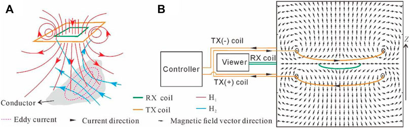
FIGURE 1. Schematic diagram of the TEM working principle. (A) Central loop device and the electromagnetic induction process of TEM coils. (B) OCTEM device diagram and magnetic field distribution in space after the reverse power supply. The receiving coil indicated by green is located at the zero-flux surface.

The nano-TEM involving a central loop device, as the conventional TEM adopted in this study, is a shallow detection method that is widely used. This device is a simplification of TEM devices without reducing measurement accuracy (Zonge International Inc., 2015). It is characterized by a high resolution, small volume effect, and suitable coupling with the target detector. The instrument used is the GDP-32II electrical method workstation produced by Zonge Engineering and Research Organization, Inc. (1992). The calculation equations for the apparent resistivity and apparent depth are as follows:

${\rho }_s=\frac{{\mu }_0}{4\pi }{\left(\frac{2{\mu }_{0}NSns}{5}\right)}^{2/3}\cdot t^{-\frac{5}{3}}{\left[\frac{I}{V\left(t\right)}\right]}^{2/3}(1)$

where ${\rho }_s$ is the apparent resistivity (Ω·m), ${\mu }_0=4\pi \times {10}^{-7}$ N/A² is the permeability of vacuum, N is the number of transmitting coil turns, S is the single-turn transmitting coil area (m²), n is the number of receiving coil turns, s is the single-turn receiving coil area (m²), t is the time (ms), I is the transmitting current (A), and V (t) is the induced electromotive force generated in the receiving coil $\left(\mu V\right)$.

$h_s={\left[\frac{3M_{s}q}{16\pi V,\left(t\right)S_{\tau }}\right]}^{\frac{1}{4}}-\frac{t}{{\mu }_{0S_{\tau }}}(2)$

where $h_s$ is the apparent depth (m), $M_s$ is the transmitting magnetic moment $\left(A\cdot m^2\right)$, $q$ is the effective area of the receiving coil (m²), $V,\left(t\right)$ is the induced voltage value observed at time t $\left(\mu V\right)$, and $S_{\tau }$ is the longitudinal conductance (S/m).

The instrument used in this OCTEM study is the HPTEM-18 device produced by Hunan 5D Geophyson Co., Ltd. (http://www.5dgeo.cn/). The calculation equation for the apparent resistivity used to process OCTEM data is as follows:

${\rho }_a={\left(\frac{I\cdot A_R\cdot A_T}{V}\right)}^{2/3}\cdot {\left(\frac{1}{t}\right)}^{5/3}\cdot 6.3219E-3(3)$

where I is the transmitting current (A), A_R is the receiving coil area (m²), A_T is the transmitting coil area (m²), t is the time (µs), and ${\rho }_a$ is the apparent resistivity (Ω·m). The algorithm can qualitatively analyze abnormal bodies at a horizontal position along the direction of the survey line.

Overview of permafrost in the study area

Permafrost in Mahan Mountain, Lanzhou, China, is the only preserved permafrost found on the Loess Plateau of China (Xie et al., 2013). It has the characteristics of small distribution area, high temperature, and small thickness (Qiu et al., 1994). Therefore, it is very sensitive to climate change and is known as a living fossil of permafrost research on the Loess Plateau (Xie et al., 2013). The peak of Mahan Mountain is 3,670.3 m above sea level, while permafrost is distributed within the range of 3,500–3,650 m above sea level (Figure 2). The annual average temperature is −2.3°C, the annual precipitation is 494 mm (Li, 1986), and the annual average surface temperature is approximate −0.23°C (Xie et al., 2013). In 1985, permafrost was discovered in Mahan Mountain for the first time, namely, a 12-m-thick permafrost layer in the exposed stratum of a shady slope artificial quarry at an altitude of 3,630 m. The thickness of the active layer ranges from 2.5 to 3.0 m, in which water exists in the form of bedrock fissure ice, and the thickness of the pure ice layer reaches up to 5–10 cm (Li, 1986), which is very rare in the high mountains of western China. In 1993, Li and Li (1993) arranged boreholes in Xiaohutan, Doulingou, Honghagou, and Tudixian for drilling investigation. According to survey data, the area of permafrost in Xiaohutan is approximately 0.15 km², which is roughly consistent with the distribution of well-developed hummocks on the surface. The permafrost thickness ranges from 5–30 m, the active layer thickness (ALT) is approximately 1.5 m, the ALT in the boundary area is only 1.2 m, and only more than 10 square meters and approximately 3-m-thick permafrost in Honghagou is retained. While there is a notable difference between Doulingou and Tudixian, certain areas contain permafrost, while others do not. They proposed that the distribution of permafrost in this area is very complex. From 2008 to 2009, Xie et al. (2010, 2013) conducted a new survey in the area where Li and Li (1993) had previously arranged boreholes. According to their results, permafrost was found only in Xiaohutan. It was speculated that the permafrost in other areas may have been completely degraded (Xie et al., 2013). According to the distribution of hummocks on the surface, it was considered that the area of permafrost was reduced from 0.15 to 0.13 km² (Xie et al., 2013). In recent years, researchers have applied the TEM, ground-penetrating radar (GPR), borehole temperature measurement, model analysis, and other methods to study permafrost in Mahan Mountain (Dong, 2013; Liu et al., 2015b; Yang et al., 2019). It is considered that the permafrost in Mahan Mountain is only distributed in Xiaohutan with a distribution area of approximately 0.11 km² and a thickness from 20–30 m, which is considered to occur in a state of rapid degradation.

FIGURE 2

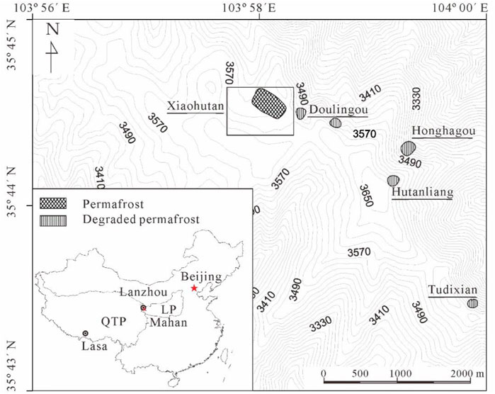
FIGURE 2. Location map of Mahan Mountain and the permafrost distribution. QTP indicates the Qinghai–Tibet Plateau; LP indicates the Loess Plateau.

According to the investigation of Li and Li (1993) and Xie et al. (2010, 2013), the minimum temperature of permafrost in Mahan Mountain reaches −0.2°C at depths from 10 to 16 m, and the upper and lower depths rise at a rate of 0.01°C/m, which is typical of high-temperature permafrost. At present, there are seven temperature measurement boreholes distributed in the study area (Figure 3), which are all distributed in and near Xiaohutan. Among them, boreholes 2, 3, 4, and 5 are located in the distribution range of permafrost, and boreholes 1, 6, and 7 are located in non-permafrost areas. We regularly monitored the ground temperature at different depths via a high-precision thermistor with an accuracy of 0.03°C. Figure 4 shows the temperature measurement curves for seven boreholes. According to the ground temperature monitoring results, the temperature of permafrost in the area is generally higher than −0.2°C, the thickness of permafrost generally approaches or exceeds 20 m, and the maximum thickness is approximately 30 m. The temperature measurement results for boreholes 2, 4, and 5 show a slight warming trend. The ground temperature in borehole 2 at the edge of permafrost is close to 0°C, and the ground temperature in borehole 4 at the center of permafrost in Xiaohutan is the lowest. The temperature changes slowly in permafrost and rapidly in bedrock.

FIGURE 3

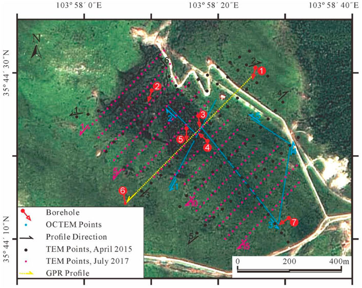
FIGURE 3. Satellite map of the Mahan Mountain permafrost region and geophysical exploration work location.

FIGURE 4

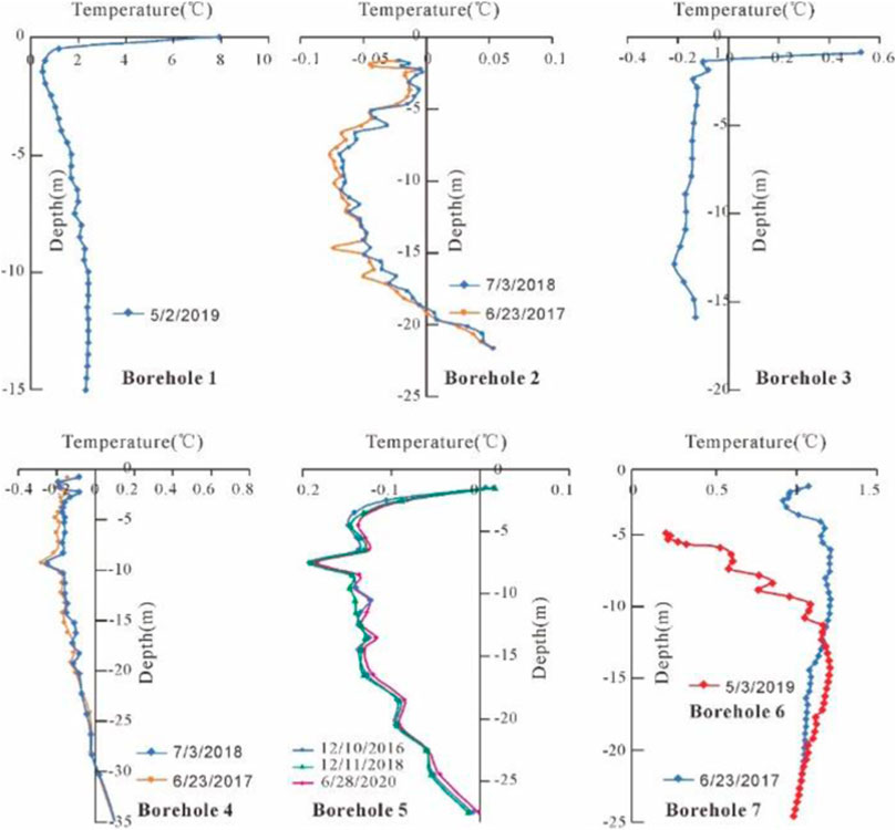
FIGURE 4. Mahan Mountain borehole temperature measurement curve.

The strata in this area mainly include the Presinian Mahan Group. The lithology is mainly composed of various migmatites, followed by gneiss, schist, and marble. The bedrock is generally buried shallowly. According to field outcrop and borehole data, the thickness of the unconsolidated sedimentary layer in Mahan Mountain generally ranges from 0.7 to 1.5 m, and the sedimentary layer gradually thickens with decreasing altitude. However, in the Xiaohutan depression, where developed permafrost, the unconsolidated sedimentary layer thickens from the smallest value of 1.2 m at the edge to the center and can reach 8 m at the thickest location at the center of the depression. The weathering degree of the upper part of the underlying bedrock is high, and permafrost is mainly developed in voids in this broken bedrock. With increasing depth, the weathering degree decreases, and the ice content in permafrost also decreases. Figure 5 shows the stratigraphic characteristics of this typical layer in the Xiaohutan depression for boreholes 3 and 5. Obviously, the difference between the permafrost in Mahan Mountain and that in most areas is the lower part of the permafrost is completely developed in bedrock and the fragmentation degree of bedrock controls the ice content in permafrost.

FIGURE 5

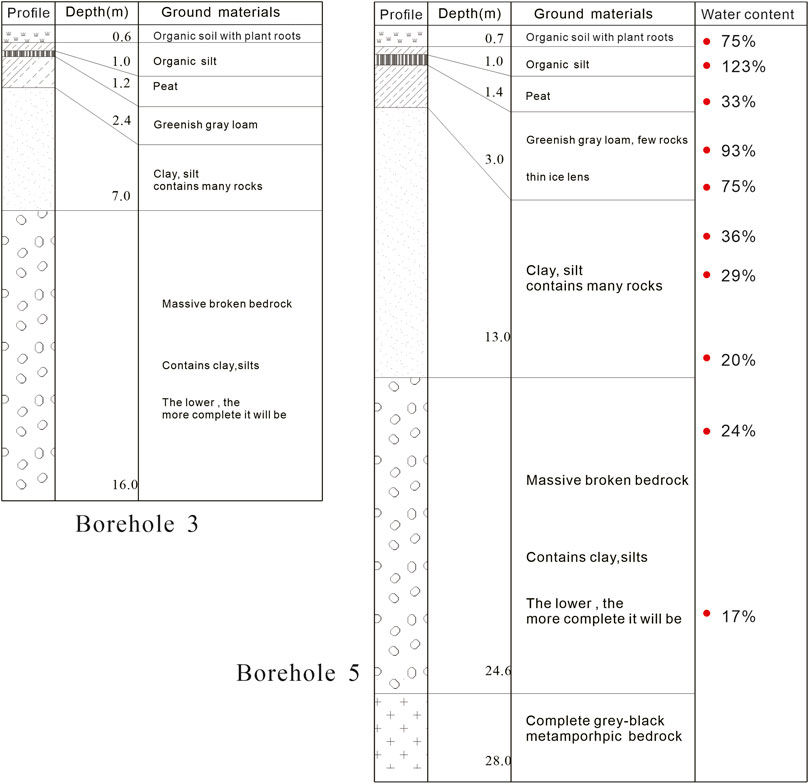
FIGURE 5. Observation map of the strata and water content in boreholes 3 and 5 in Mahan Mountain.

Obviously, the electrical changes in the strata in this area are mainly determined by the water conditions in the voids of the broken bedrock and the thickness of the loose sedimentary layer. The loose layer in the upper part of the formation contains more water storage structures and more suitable surface water conditions, so the surface obviously exhibits low resistivity. The lower permafrost is mainly distributed in the weathered broken layer of bedrock, so it exhibits a higher resistivity than that of the upper layer. In addition, the development of solid ice can theoretically produce a higher resistivity than that of the surrounding strata at the same depth. At the lower surface and boundary of permafrost, because the horizontal formation components change slightly, only the existing form of water changes. The area of the meltwater distribution differs from that of permafrost with solid ice. The formation is deeper, the bedrock tends to be complete, and the resistivity value tends to remain stable. Based on the abovementioned understanding, in this study, the formation resistivity change caused by other small changes is ignored, and it is considered that all resistivity differences are caused by water change.

Data acquisition

Nano-TEM detection at 94 measuring points (black dots in Figure 3) was conducted in Xiaohutan of Mahan Mountain in Lanzhou in April 2015, with a point spacing of 50 m, forming six detection profiles. In July 2017, 12 profiles with 273 measuring points (pink dots in Figure 3) were remeasured with the same detection parameters and 20 m as the point spacing. To ensure more accurate detection results, the total station was used to accurately locate the measurement points. The measurements were repeated three–five times at each point. In June 2018, single-point nano-TEM sounding was conducted in many areas in Mahan Mountain. In July 2020 and September 2020, an HPTEM-18 equivalent anti-magnetic flux transient electromagnetic system based on the OCTEM principle was used twice to complete five detection profiles in the permafrost area of Mahan Mountain, with a total of 294 measurement points (blue dots in Figure 3). The locations of these measurement profiles are also shown in Figure 3, and the spacing between the measurement points is 5 m. Among these profiles, profile 1 passes through the permafrost distribution area, profile 2 is in the permafrost area, half of profile 3 passes through the permafrost distribution area, and profiles 4 and 5 are located in the hummock degradation area at the permafrost boundary. Table 1 lists the actual detection parameters.

TABLE 1

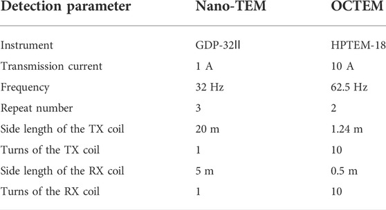
TABLE 1. Detection parameters used in the nano-TEM and OCTEM.

Data processing

During nano-TEM data processing, the three measured datasets with the most similar measurement results were selected to participate in the calculation to ensure that the results reduced the random interference as much as possible. STEMNV software was used for two-dimensional fitting with a layered stratum model. The OCTEM uses multiple stacking steps (more than 300 times) to improve the signal-to-noise ratio, and HPTEM-18 data processing software was used to process the measured data. In the process of data processing, unreasonable measured data could be corrected and eliminated at any time to ensure the reliability of the data processing results. After the data calculation step, all the data of this study were compiled into profiles in Surfer software (www.goldensoftware.com), and the agreed color scheme was used.

Detection results

Before the discovery of permafrost in Mahan Mountain, scholars conducted resistivity sounding exploration in the peak area of Mahan Mountain to determine whether permafrost had developed and remained. Due to the shallow distribution of bedrock in Mahan Mountain and the high resistivity of bedrock close to frozen soil, the detection results (Figure 6) did not identify the existence of frozen soil (Guo, 1982). When the semipolar distance AB/2 ranges from 1.5–6 m, the apparent resistivity value of the formation increases obviously, but the amplitude is small. Now, we know that the determined high-resistivity anomaly is permafrost. Therefore, it is speculated that there is little difference between the resistivity values of permafrost and underlying bedrock in this area. According to Hauck and Muhll (1999b), and Hauck et al. (2003), this occurs because DC detection is affected by the upper stratum, and the greater the detection depth is, the smaller the difference in resistivity will be. However, the difference is that TEM detection involves the induction of the primary field within a specific layer at a certain time, so the formation itself slightly impacts TEM detection, and the TEM can measure more obvious differences in formation resistivity. Figure 6 also shows that the resistivity of Mahan Mountain permafrost reaches as low as 200–300 Ω m. In fact, the resistivities of the weathered bedrock, surface melting layer, and surface freezing layer were also measured, reaching approximately 600, 25, and 80 Ω m, respectively, at −3°C and 4,800 Ω m at −13°C, which is consistent with the results measured under DC conditions (Yang et al., 2019). In this study, the reference resistivity of the surface melting layer was selected as 25 Ω m.

FIGURE 6

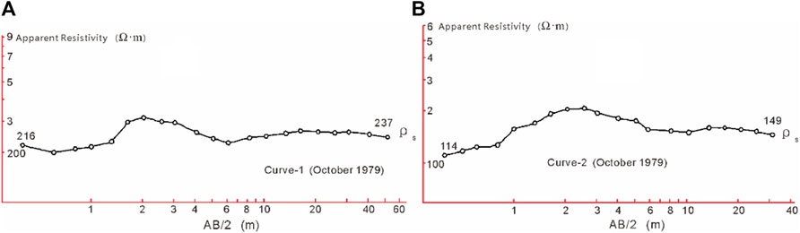
FIGURE 6. Two permafrost DC sounding curves of Mahan Mountain. (A) located on the top of the mountain with thin loose layer and higher apparent resistivity value; (B) located slightly lower with thick loose layer and lower apparent resistivity value.

Nano-TEM measurement

The final inversion results show low-resistivity anomalies in the profile; in combination with the satellite image depicted in Figure 3, it can be found that these anomalies are consistent with the distribution of surface wetlands (the dark area in Figure 3 is the Xiaohutan depression, and hummocks are more notably developed in the dark area), and there is no longitudinal change in the profile within 15 m. The measured permafrost depth in the four boreholes located in the permafrost range is no more than 30 m, while the inversion results cannot significantly detect the low-resistivity characteristics of the lower limit of permafrost within 40 m. Choosing profile 2 detected in April 2015 as an example (Figure 7), we can find low-resistivity anomalies at 100 and 500 m, while these two locations signify the boundary of the distribution of hummocks at the surface. If the hummocks on the surface are consistent with the distribution of permafrost, 100 and 500 m represent the boundaries of permafrost. Through comparison of Figures 3 and 7, it can be found that the 100–500 m section in the satellite map is a continuous hummock area and a continuous geological body with medium- and high-resistivity values in the TEM profile, which is consistent with the boundary characteristics of permafrost. Before this study, the distribution range of permafrost in Mahan Mountain was obtained according to drilling results and the development range of surface hummocks, but there are no continuous observation data to prove that this approach is correct. In addition, at a depth of approximately 15 m, there is an obvious shallow detection blind area, which shows low resistivity and is inconsistent with the high resistivity of permafrost. Borehole 2 is approximately 50 m away from the 300-m location (Figure 3). The temperature measurement results show that the temperature reaches 0°C at a depth of approximately 19 m, which suggests that the thickness of permafrost here is approximately 20 m (Figure 4), which is not found from the TEM results.

FIGURE 7

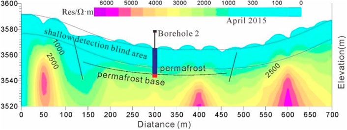
FIGURE 7. Nano-TEM sounding profile 2 of Mahan Mountain, April 2015.

Does the abovementioned occur because the spacing between the survey points is too large, resulting in the lack of profile continuity? The detection results obtained low-resistivity anomalies along the profile consistent with the boundary distribution of surface wetlands, but anomalies remain that are inconsistent with the continuity characteristics of frozen soil in the possible permafrost distribution area. Choosing profile 7 detected in July 2017 (Figure 8A) as another example, the spacing of the measuring points was 20 m. Through specific analysis of the profile, it can be observed that low-resistivity anomalies are obvious where the measuring points are missing. However, there is still an obvious shallow detection blind area after the spacing of the measuring points is improved, while there is still no change in the identification of the permafrost base. We speculate that anomalies may be caused by fractures in the bedrock and distribution of groundwater. However, in terms of lower limit identification of permafrost, reducing the distance between measurement points still fails to clearly detect the water characteristics at the lower boundary of permafrost. Theoretically, to eliminate this problem in the shallow layer, increasing the number of turns of the measuring coil can suppress random interference and improve the signal-to-noise ratio and fidelity. In June 2018, the other test parameters remained unchanged. We measured and compared the number of turns of the transmitting and receiving coils in this area. The results show that increasing the number of turns of the transmitting coil slightly affects the detection results, while reducing the coil size decreases the detection depth.

FIGURE 8

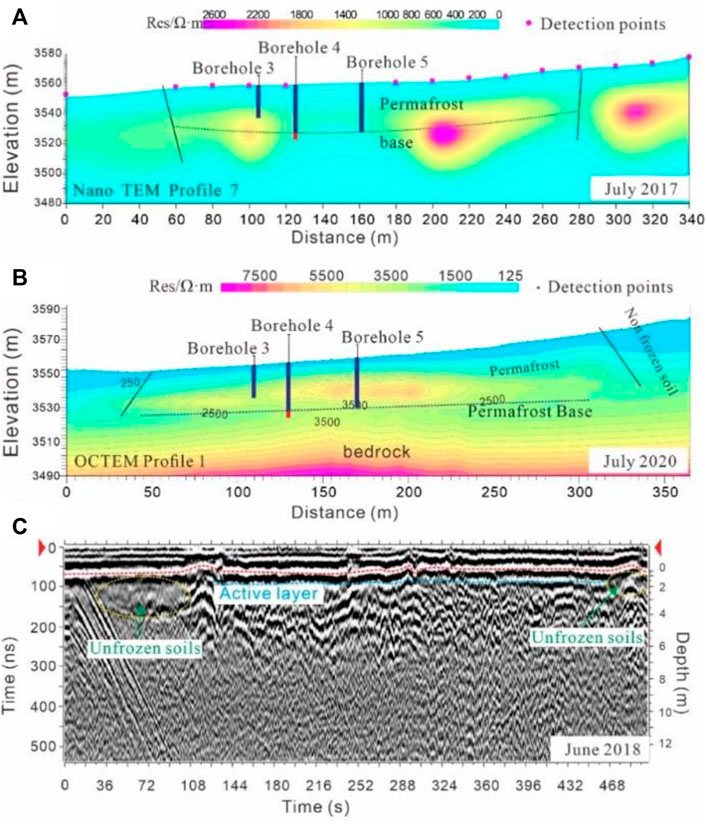
FIGURE 8. Comparison of the nano-TEM, OCTEM, and GPR methods in identifying permafrost in the shallow bedrock area of Mahan Mountain. (A) Nano-TEM profile with a 20-m point spacing. (B) OCTEM profile with a 5-m point spacing. (C) 50-MHz GPR detection profile.

Through the abovementioned experiments, it can be concluded that the nano-TEM shows an obvious shallow detection blind area in the exploration of permafrost in Mahan Mountain, Lanzhou, although this method achieves a certain identification ability regarding the boundary of permafrost but cannot effectively identify the permafrost base.

Opposing coils transient electromagnetic method measurement

OCTEM exploration profile 1 (Figure 8B) extends from northeast to southwest, with a total of 72 measuring points and a total length of 365 m (Figure 3). The surface enters the Xiaohutan depression with hummock distributions from 45 to 320 m, and hummocks then disappear, which is consistent with the high-resistivity distribution detected by the OCTEM. The hummocks within 100–245 m below the ground surface are well-developed and dark in color. The hummocks on both sides are degraded outward, which is also very obvious in the OCTEM profile. In the OCTEM profile, the resistivity value in this section is significantly higher than that on both sides. Under the condition that the lateral conditions of the formation are similar, the reason for this difference in lateral resistivity is the differential distribution of conductive substances in the formation. It is believed that the distribution difference of the water resistivity is small only when the bedrock remains relatively shallow buried in the permafrost area for many years. The profile shows that there is an obvious low-resistivity distribution layer at depths above 3,526 m above sea level, and the depth of this layer varies between 25 and 30 m, which coincides with the lower limit depth of permafrost obtained via borehole and ground temperature monitoring. Permafrost degradation dissolves solid ice in bedrock voids, and part of the meltwater flows away from the rock voids. At the same time, water is adsorbed by silt, clay, and other particles in the formation or accumulates in unconnected rock pores so that the resistivity at the lower limit and boundary of permafrost is lower than that of permafrost. At an elevation of 3,526 m in the figure, the resistivity is lower than that of the upper and lower strata, which is in line with the low-resistivity characteristics of meltwater at the permafrost boundary. By comparing the nano-TEM (Figure 8A) and GPR results (Figure 8C) at similar locations (Figure 3), it can be found that the OCTEM is the most intuitive and accurate method for identifying permafrost bases and boundaries.

OCTEM profile 2 (shown in Figure 9) is located in the central area of the Xiaohutan depression, with 31 measuring points from southeast to northwest, and the length of the profile is 150 m. The surface contains well-developed hummocks (Figure 10A), and the surface soil is saturated with water. It can be found that there is a high-resistivity layer with a thickness from 25 to 30 m above the bedrock from the beginning to the end. This layer slowly thins from the center of the depression (the starting point of profile 2, near borehole 4) to the edge, but the change range is small. The thickness of the high-resistivity layer at the end is reduced to 20 m. Borehole 4 at the starting point shows that the thickness of permafrost here is approximately 28 m, and the thickness of permafrost at the end is approximately 22 m, which agrees with the temperature measurement results in borehole 2 (the distance between borehole 2 and the end of profile 2 is approximately 65 m).

FIGURE 9

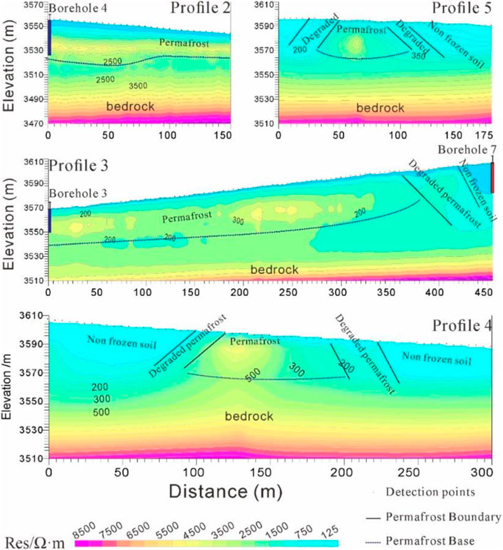
FIGURE 9. OCTEM sounding profiles in Mahan Mountain.

FIGURE 10

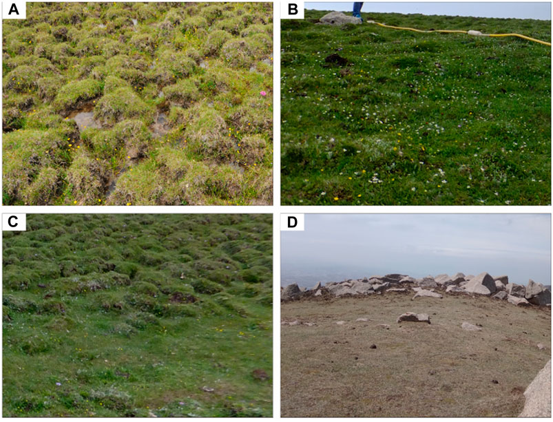
FIGURE 10. Photos of surface vegetation in the Mahan Mountain area. (A) In the permafrost region, shot at location a in Figure 11. (B) Non-permafrost region, shot at location b in Figure 11. (C) Degraded permafrost region, shot at location c in Figure 11. (D) Bedrock exposed area, shot at the top of the mountain.

OCTEM profiles 3, 4, and 5 (Figure 9) show permafrost boundary test results. Profile 3 starts from the central area of the permafrost distribution and passes through the permafrost area along the southeast direction. The hummocks on the surface degenerate from 380 m along profile 3 and disappear at 420 m (Figure 10B shows that the surface hummocks have been completely degraded), which is strictly consistent with the high-resistivity anomaly detected. The high-resistivity anomaly exhibits a clear low-resistivity lower interface, which shows obvious permafrost base characteristics. Profiles 4 and 5 both have sparse hummocks in the middle, and the hummocks on both sides are completely degraded (Figure 10C shows the obvious boundary of the surface meadow). All the high-resistivity layers in the OCTEM profiles are clear, and the location of the high-resistivity anomaly is consistent with the distribution of surface hummocks. Profile 3 has a relatively stable distribution of high resistivity values, with clear low resistivity values at the lower interface, and the depth varies between 23 and 29 m. From 380 to 420 m, the hummocks are sparsely distributed and seriously degraded and disappear completely at 420 m. The section shows that the resistivity is slightly higher than that in the melting area, and the boundary with the melting area is clear. It is speculated that the permafrost in this section occurs in the degraded state and contains more meltwater than does the non-degraded permafrost. However, because solid ice has not completely melted, the resistivity is higher than that in the melting area. The normal annual temperature measurement result for borehole 7 at the end of the survey line is positive (Figure 4), which is consistent with the detection result. Along the direction of Profile 3, at the top of the mountain about 180 m away from the end of Profile 3, the vegetation is almost completely degraded and massive bedrock is exposed (Figure 10D). Profile 4 (95–200 m) and profile 5 (15–95 m) show continuous high-resistivity anomalies with clear lower interfaces. It should be noted that obvious changes in hummocks appear on the surface at these two locations. The hummocks on the surface are only distributed from 90 to 205 m along profile 4 and are only distributed from 10 to 120 m along profile 5.

Through the aforementioned analysis, in the area measured by the OCTEM in this study, the thickness of permafrost generally varies between 20 and 30 m and has a clear boundary and base characteristics, which directly confirms the corresponding relationship between permafrost and hummock distribution. According to this correspondence, combined with satellite images and actual survey data, we mapped the distribution range of permafrost in Maxian Mountain (closed area of the yellow line in Figure 11). In contrast to previous work, this study identified a region where permafrost occurs in a degraded state but is not yet completely degraded (the area between the brown and yellow lines in Figure 11).

FIGURE 11

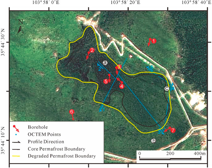
FIGURE 11. Distribution range of permafrost in Mahan Mountain based on geophysical exploration and surface vegetation characteristics.

Conclusion

By comparing the application of the nano-TEM and OCTEM, it can be found that there is an obvious detection blind area in the exploration of permafrost in Mahan Mountain with the conventional TEM, and it is difficult to distinguish permafrost vertically developed in bedrock. However, the OCTEM can effectively eliminate the primary field interference, so this method attains a higher detection accuracy and can observe small changes in the formation water content horizontally and vertically to identify the spatial distribution of permafrost. In addition, through this comparative experiment, new insights into the distribution of permafrost in Mahan Mountain are obtained. For the first time, the observation results confirm that the distribution of surface hummocks in this area is consistent with that of permafrost and degraded hummocks indicate permafrost degradation.

Previously, the distribution area of permafrost in Mahan Mountain was considered to be degraded to 0.13 km². However, now, the actual distribution area of permafrost has not reached this value, but the boundary area is obviously degrading. Meltwater has accumulated in the degraded area, showing the distribution characteristics of the core area–degraded area–completely degraded area from the center toward the outside. According to the distribution statistics of hummocks on the surface, at present, the distribution area of the permafrost core area in Mahan Mountain is only 0.11 km², with an outer circumference of approximately 0.04 km. The area with a sparse distribution of surface hummocks occurs in a state of rapid degradation, and obvious water characteristics can be detected in the strata.

Although the OCTEM eliminates the primary field interference, solves the problem of shallow detection blind areas, and detects the permafrost distribution in shallow bedrock in the Mahan Mountain area, this does not indicate that this method can effectively detect permafrost in all shallow bedrock areas. The OCTEM is particularly sensitive to water content. The permafrost in the Mahan Mountain area is typical high-temperature permafrost, and there is water accumulation in both the boundary area and permafrost base, so permafrost can be detected and identified. However, many permafrost zones in shallow bedrock areas do not exhibit similar conditions. Therefore, more research is needed on whether the OCTEM can identify low-temperature permafrost in shallow bedrock areas.

Data availability statement

The raw data supporting the conclusion of this article will be made available by the authors, without undue reservation.

Author contributions

TW, XW, and CX contributed to the conception of the study, supervision, and funding acquisition; GY: contributed to literature synthesis and wrote the manuscript; GL, WW, and YZ provide field actual measurement and helped perform the analysis with constructive discussions.

Funding

This work was supported by the Strategic Priority Research Program of Chinese Academy of Sciences (XDA23060703); the National Natural Science Foundation of China (41671068); and the State Key Laboratory of Cryospheric Science (SKLCS-ZZ-2022).

Acknowledgments

We thank Wei Xu from the 149 Team of Gansu Coalfields Geological Bureau for providing instruments and field guidance for this study, and collecting OCTEM data in person, as well as providing guidance for later data processing.

Conflict of interest

The authors declare that the research was conducted in the absence of any commercial or financial relationships that could be construed as a potential conflict of interest.

Publisher’s note

All claims expressed in this article are solely those of the authors and do not necessarily represent those of their affiliated organizations, or those of the publisher, the editors, and the reviewers. Any product that may be evaluated in this article, or claim that may be made by its manufacturer, is not guaranteed or endorsed by the publisher.

References

Barsukov, P. O., and Fainberg, E. B. (2013). Three-dimensional interpretation of TEM soundings. Izv. Phys. Solid Earth 49 (4), 517–525. doi:10.1134/S1069351313040022

CrossRef Full Text | Google Scholar

Christiansen, A. V., Auken, E., and Sørensen, K. (2006). “The transient electromagnetic method,” in Groundwater geophysics (Berlin, Heidelberg: Springer), 179–225. doi:10.1007/3-540-29387-6

CrossRef Full Text | Google Scholar

Danielsen, J. E., Auken, E., Jørgensen, F., Søndergaard, V., and Sørensen, K. I. (2003). The application of the transient electromagnetic method in hydrogeophysical surveys. J. Appl. Geophys. 53 (4), 181–198. doi:10.1016/j.jappgeo.2003.08.004

CrossRef Full Text | Google Scholar

Dong, X. C. (2013). Characteristics of surface energy budget components in permafrost region of the Mahan Mountain, Lanzhou. J. Glaciol. Geocryol. 35 (2), 320–326. doi:10.7522/j.issn.1000-0240.2013.0038

CrossRef Full Text | Google Scholar

Guo, D. X. (1982). Preliminary approach to the existence of permafrost in Mahan mountain area, Lanzhou. J. Glaciol. Geocryol. 4 (4), 63–66. (in Chinese)

Google Scholar

Harada, K., Wada, K., and Fukuda, M. (2000). Permafrost mapping by transient electromagnetic method. Permafr. Periglac. Process. 11 (1), 71–84. doi:10.1002/(SICI)1099-1530(200001/03)11:1<71::AID-PPP339>3.0.CO;2-#

CrossRef Full Text | Google Scholar

Harada, K., Wada, K., Sueyoshi, T., and Fukuda, M. (2006). Resistivity structures in alas areas in Central Yakutia, Siberia, and the interpretation of permafrost history. Permafr. Periglac. Process. 17 (2), 105–118. doi:10.1002/ppp.551

CrossRef Full Text | Google Scholar

Harris, C., Haeberli, W., Mühll, D. V., and King, L. (2001). Permafrost monitoring in the high mountains of europe: The PACE project in its global context. Permafr. Periglac. Process. 12 (1), 3–11. doi:10.1002/ppp.377

CrossRef Full Text | Google Scholar

Hauck, C. (2001). Geophysical methods for detecting permafrost in high mountains. PhD thesis ETH Zurich 171, 204.

Google Scholar

Hauck, C., Guglielmin, M., Isaksen, K., and Vonder Mühll, D. (2001). Applicability of frequency‐domain and time‐domain electromagnetic methods for mountain permafrost studies. Permafr. Periglac. Process. 12 (1), 39–52. doi:10.1002/ppp.383

CrossRef Full Text | Google Scholar

Hauck, C., Mühll, D. V., and Maurer, H. (2003). Using DC resistivity tomography to detect and characterize mountain permafrost. Geophys. Prospect. 51 (4), 273–284. doi:10.1046/j.1365-2478.2003.00375.x

CrossRef Full Text | Google Scholar

Hauck, C., and Mühll, D. V. (1999a). Detecting alpine permafrost using electro-magnetic methods. Adv. Cold-Region Therm. Eng. Sci. 533, 475–482. doi:10.1007/BFb0104205

CrossRef Full Text | Google Scholar

Hauck, C., and Mühll, D. V. (1999b). “Using DC resistivity tomography to detect and characterise mountain permafrost,” in Proceeding of the 61st EAGE Conference and Exhibition, June 1999 (Helsinki, Finland: European Association of Geoscientists and Engineers). doi:10.3997/2214-4609.201407626

CrossRef Full Text | Google Scholar

Henderson, J. D. (1980). “Permafrost mapping along transportation corridors,” in Proc. Symp. Permafrost geophysics (Techn. Memorandum), 128, 130–138. (No. 5).

Google Scholar

Hoekstra, P. (1973). “Electromagnetic probing of permafrost,” in Proceedings of 2nd International Conference on Permafrost (Yakutsk, USSR: North American Contribution), 517–526.

Google Scholar

Ji, Y. J., Lin, J., Yu, S. B., Wang, Z., and Wang, J. (2006). A study on solution of transient electromagnetic response during transmitting current turn‐off in the ATTEM system. Chin. J. Geophys. 49 (6), 1718–1725. doi:10.1002/cjg2.1000

CrossRef Full Text | Google Scholar

King, L., Fisch, W., Haeberli, W., and Wächter, H. P. (1987). A sensory-integrative approach to the education of the autistic child. Occup. Ther. Health Care 23 (2), 77–85. doi:10.1080/J003v04n02_08

PubMed Abstract | CrossRef Full Text | Google Scholar

Kuzmin, P. V., and Morrison, E. B. (2014). U.S. Patent No. 8,786,286. Washington, DC: U.S. Patent and Trademark Office.

Google Scholar

Li, S. D. (1986). Permafrost found on maxian mountains near Lanzhou. J. Glaciol. Geocryol. 8 (4), 409–410. (in Chinese)

Google Scholar

Li, Z. F., and Li, S. D. (1993). Regional features of permafrost in Mahan Mountain and their relationship to the environment. J. Glaciol. Geocryol. 15 (001), 83–89. (In Chiese).

Google Scholar

Liu, G. Y., Wang, W., Zhao, L., Chen, J., Pang, Q. Q., Wang, Z. W., et al. (2015a). Using transient electromagnetic method to sound permafrost depth in the West Kunlun Mountains. J. Glaciol. Geocryol. 37 (1), 38–48. doi:10.7522/j.issn.1000-0240.2015.0004

CrossRef Full Text | Google Scholar

Liu, W. H., Xie, C. W., Zhao, L., Wu, T. H., Li, R., Wang, W., et al. (2015b). Simulating the active layer depth and analyzing its influence factors in permafrost of the Mahan Mountain, Lanzhou. J. Glaciol. Geocryol. 37, 1443–1452. doi:10.7522/j.isnn.1000-0240.2015.0160

CrossRef Full Text | Google Scholar

McNeill, J. D. (1991). PROTEM-47 Transient electromagnetic system manual. www.geonics.com.

Google Scholar

Mühll, D. V., Hauck, C., Gubler, H., McDonald, R., and Russill, N. (2001). New geophysical methods of investigating the nature and distribution of mountain permafrost with special reference to radiometry techniques. Permafr. Periglac. Process. 12 (1), 27–38. doi:10.1002/ppp382

CrossRef Full Text | Google Scholar

Mühll, D. V., Hauck, C., and Gubler, H. (2002). Mapping of mountain permafrost using geophysical methods. Prog. Phys. Geogr. Earth Environ. 26 (4), 643–660. doi:10.1191/0309133302pp356ra

CrossRef Full Text | Google Scholar

Nabighian, M. N. (1984). Foreword and introduction. Geophysics 49 (7), 849–853. doi:10.1190/1.1441730

CrossRef Full Text | Google Scholar

Nabighian, M. N., and Macnae, J. C. (1991). Time domain electromagnetic prospecting methods. Electromagn. Methods Appl. Geophys. 2, 427–520. doi:10.1190/1.9781560802686

CrossRef Full Text | Google Scholar

Qiu, G. Q., Liu, J. S., and Liu, H. X. (1994). Geocryological glossary. Lanzhou: Gansu Science and Technology Press. (in Chinese).

Google Scholar

Smith, R. S., and Balch, S. J. (2000). Robust estimation of the band-limited inductive-limit response from impulse-response TEM measurements taken during the transmitter switch-off and the transmitter off-time: Theory and an example from Voisey’s Bay, Labrador, Canada. Geophysics 65 (2), 476–481. doi:10.1190/1.1444741

CrossRef Full Text | Google Scholar

Szarka, L. (1988). Geophysical aspects of man-made electromagnetic noise in the Earth — a review. Surv. Geophys. 9, 287–318. doi:10.1007/BF01901627

CrossRef Full Text | Google Scholar

Telford, W. M., Geldart, L. P., and Sheriff, R. E. (1991). Applied geophysics. Cambridge: Cambridge University Press.

Google Scholar

Walker, S., and Rudd, J. (2009). Extracting more information from on-time data. ASEG Ext. Abstr. 2009 (1), 1–8. doi:10.1071/ASEG2009ab053

CrossRef Full Text | Google Scholar

Wang, W., Liu, G. Y., Yu, Q. H., and Sheng, Y. (2011a). Geophysical mapping permafrost using TEM. J. Glaciol. Geocryol. 33 (1), 156–163. doi:10.1007/s12182-011-0118-0

CrossRef Full Text | Google Scholar

Wang, T., Yu, Q. H., You, Y. H., Wang, W., and Du, E. J. (2011b). The application of electromagnetic technology to permafrost exploration. Geophys. Geochem. Explor. 35 (5), 638–642. doi:10.1002/(SICI)1099-1530(200001/03)11:13.0.CO;2-#

CrossRef Full Text | Google Scholar

Xi, Z., Long, X., Huang, L., Zhou, S., Song, G., Hou, H., et al. (2016a). Opposing-coils transient electromagnetic method focused near-surface resolution. Geophysics 81 (5), E279–E285. doi:10.1190/Geo2014-0564.1

CrossRef Full Text | Google Scholar

Xi, Z., Long, X., Huang, L., Zhou, S., Gang, S., Hai-Tao, H., et al. (2016b). Opposing coils transient electromagnetic method for shallow subsurface detection. Chin. J. Geophys. 59 (9), 551–559. doi:10.1002/cjg2.30006

CrossRef Full Text | Google Scholar

Xie, C. W., Zhao, L., Wu, J. C., and Qiao, Y. P. (2010). Features and changing tendency of the permafrost in mahan mountain, Lanzhou. J. Glaciol. Geocryol. 32 (5), 893–890. doi:10.3724/SP.J.1231.2010.06586

CrossRef Full Text | Google Scholar

Xie, C., Gough, W. A., Tam, A., Zhao, L., and Wu, T. (2013). Characteristics and persistence of relict high‐altitude permafrost on Mahan Mountain, loess plateau, China. Permafr. Periglac. Process. 24 (3), 200–209. doi:10.1002/ppp.1776

CrossRef Full Text | Google Scholar

Xue, G. Q., Li, X., and Di, Q. Y. (2007). The progress of TEM in theory and application. Prog. Geophys. 22 (4), 1195–1200. doi:10.1016/S1872-5791(08)60015-9

CrossRef Full Text | Google Scholar

Yang, G. Q., Xie, C. W., Wang, W., Du, E., Liy, W., Zhang, Y., et al. (2019). Study on TEM sounding permafrost with shallow bedrock. J. Glaciol. Geocryol. 41 (5), 1067–1077. doi:10.7522/j.issn.1000-0240.2019.0328

CrossRef Full Text | Google Scholar

Zonge Engineering and Research Organization, Inc (1992). Introduction to TEM. Extracted from practical geophysics II: Northwest mining association.

Google Scholar

Zonge International Inc (2015). NanoTEM® near-surface method. Available from: http://zonge.com/geophysical-methods/electrical-em/nanotem/ (accessed June 14, 2015).

Google Scholar