An Integrated Approach to Characterize Temporal–Spatial Variations in PM2.5 Concentrations at the Ground Level and Its Implication on Health Impact Assessments

Although PM_2.5 concentrations measured by the governmental air quality monitoring station (AQMS) have been widely used for conducting exposure assessments, it might be not able to reflect the residents’ exposures, especially for those associated with ground emissions. The present study was conducted in a city area for 1 year. A mobile monitoring station (MMS) was established to measure the PM_2.5 concentrations at the ground level. A significant linear relationship (R² = 0.53) was found between the MMS-measured concentrations and the corresponding concentrations obtained from the AQMS (15 m above the ground level), and the former was ∼ 1.11 times (95% CI: 1.08-1.15) in magnitude higher than that of the latter. To characterize the spatial variation of the area, the MMS-measured values were further classified into three different regions. A consistent trend was found in the present study for all collected data as industry region≒urban region > harbor region. The aforementioned results clearly indicate that the residents’ ambient PM_2.5 exposures do have spatial differences. Seven-year AQMS-measured concentrations (i.e., AQMS_7-yr) were used to establish the long-term PM_2.5 concentrations at the ground level (i.e., MMS_7-yr) of the three different regions using the linear regression equations obtained from the MMS and AQMS. Health impact functions and local health data were used to quantify the PM_2.5-attributable health burden for both AQMS_7-yr and MMS_7-yr, respectively. Results show that the former is ∼ 10.4% lower in magnitude than the latter in the estimated lung cancer death attributed fraction (AF). In particular, the decrease of unit PM_2.5 (μg/m³) would lead to a 0.75 and 0.71% decrease in the estimated AF of lung cancer death for AQMS_7-yr and MMS_7-yr, respectively. As a result, directly using AQMS_7-yr would lead to an underestimation of ∼ 1,000 lung cancer deaths annually in Taiwan in comparison with those using MMS_7-yr. The aforementioned results clearly indicate the importance of characterizing ground-level exposures for assessing the health impact of residents, and the methodology developed by the present study would be helpful for solving the aforementioned problem.

Introduction

It has been reported that air pollution is responsible for ∼ 2.9 million deaths per year accounting for ∼ 35% of all environmental pollution-related deaths (Fuller et al., 2019). The International Agency for Research on Cancer (IARC) has classified outdoor air pollution as Group 1 carcinogen (i.e., carcinogenic to humans) (Straif et al., 2013). Among various particulate matters (PMs), many pieces of evidence have shown that PM_2.5 (i.e., PM with a particle size less than 2.5 μm) has a much stronger impact on human health than those with greater particle sizes (Environmental Protection Agency U.S, 2019). PM_2.5 is responsible for many adverse health effects, including lung cancer, chronic obstructive pulmonary disease (COPD), ischemic heart disease (IHD), strokes, and acute lower respiratory infections (ALRIs). (Mustafic et al., 2012; Forouzanfar et al., 2016; Monrad et al., 2017). Therefore, the control of atmospheric PM_2.5 concentrations has been considered as the primary concern in many countries. However, it should be noted that the initiation of appropriate abatement strategies for PM_2.5 should start with knowing the correct PM_2.5 exposure levels and health impact on the residents in the target area. Considering the existence of the intrinsic spatial and temporal variations in residents’ PM_2.5 exposure concentrations, developing suitable exposure assessment (EA) methodologies has become an important issue in the environmental health science field.

At present, the methodologies used for conducting PM_2.5 EA can be classified into two categories: the non-ground level (also called macroenvironment) and ground level (microenvironment) (Straif et al., 2013; Dias and Tchepel, 2018; Li et al., 2018; Caplin et al., 2019; Environmental Protection Agency U.S, 2019). For non-ground-level EA methods, exposure data can be obtained from governmental air quality monitoring stations (AQMS) (i.e., fixed monitoring stations), model estimation, satellite remote sensing, etc. (Ozkaynak et al., 2013; Environmental Protection Agency U.S, 2019). The aforementioned methodologies are widely used in conducting EA on a large scale (such as on the whole country level, or even across-country level) and assuming the uniformity of PM_2.5 concentrations in each divided subarea. For example, PM_2.5 AQMS data from many countries were collected by the World Health Organization (WHO) for assessing the global exposure and health burden assuming the uniformity of PM_2.5 concentrations at a city level (W.H.O., 2012). However, the aforementioned methods might not be feasible for conducting PM_2.5 EA in a small area (such as at a city level) because the spatial heterogeneity might have a significant impact on the residents’ PM_2.5 exposure concentrations (Fishbain et al., 2017; Malings et al., 2020).

It is known that urban traffic accounts for >50% of the total PM₁₀ emissions. In comparison with PM₁₀, urban traffic has an even greater contribution to PM_2.5 concentrations at the ground level (Han and Naeher, 2006). The main traffic emission sources include road traffic, airport, and port operations (Kingham et al., 2013; Mazaheri et al., 2018). Among them, urban ground PM_2.5 concentrations are mainly influenced by road traffic contributed by both traffic exhaust and non-traffic exhaust (e.g., brake wear and road dust) (Jeong et al., 2019). Considering the proximity of residents to ground PM_2.5 emission sources (such as traffic), higher exposure concentrations at the ground level are expected than those obtained from the non-ground level (e.g., AQMS). Therefore, many methodologies have been developed to measure ground-level PM_2.5 concentrations (such as the mobile monitoring station (MMS) (Hankey and Marshall, 2015; Okokon et al., 2017; Lin et al., 2018; Cheng et al., 2019; Shen and Gao, 2019), air box (Lee et al., 2019; Lin et al., 2020), and modeling estimation (Hu et al., 2016; Jung et al., 2018)) for better characterizing residents’ exposures in the small area of interest. Although the air box and modeling methods are less expensive and provide real-time information, many limitations are involved if they are used for conducting EA, including the accuracy and reliability of the collected data (Cabada et al., 2004; Snyder et al., 2013; Castell et al., 2017; Morawska et al., 2018; Williams et al., 2019; Li et al., 2020; Zamora et al., 2020; Environmental Protection Agency U.S, 2021). For the MMS, it has been found to be more accurate and reliable than the aforementioned two methodologies. On the condition of the existence of an AQMS in the target area, the use of the MMS method provides the possibility for better characterizing spatiotemporal personal exposures in a given microenvironment by combining with the AQMS data (Hankey and Marshall, 2015; Droge et al., 2018; Piotrowicz and Polednik, 2019).

In Taiwan, at least one AQMS is installed in every city or township for characterizing PM_2.5 concentrations in different areas. Although concentrations obtained from the AQMS provide longitudinal information of the area, however, they are inadequate to characterize the residents’ PM_2.5 exposures in different regions of the area because of their intrinsic spatial heterogeneity (Borge et al., 2016). Therefore, developing new monitoring strategies with the aid of long-term AQMS data to characterize the residents’ both temporal and spatial exposures has become an important issue for conducting PM_2.5 EAs. In principle, the development of predicting models between PM_2.5 concentrations of the AQMS and MMS would be helpful for establishing the residents’ long-term PM_2.5 exposure concentrations at the ground level in different regions. However, it should be noted that before the establishment of the aforementioned predicting models, possible interference factors should be considered, including meteorological factors (e.g., temperature, humidity, (RH), wind speed, etc.) (Ye et al., 2018; Zhang et al., 2018; Lee et al., 2020; Rittner et al., 2020; Yousefian et al., 2020; Yang et al., 2022) and other co-emission pollutants (e.g., primary pollutants of NO₂, SO₂ etc. and secondary pollutants of O₃) (Saraswat et al., 2013; Zhang et al., 2018; Guo et al., 2019).

Since PM_2.5 concentration plays a significant role in human health, conducting a health impact assessment (HIA) would provide better evidence to help decision-makers for developing proper control strategies (W.H.O., 2022). For any given air pollutant, the calculation of the burden of disease (BOD) is widely adopted for conducting the HIA (van der Kamp and Bachmann, 2015; W.H.O., 2016; Maji et al., 2017; Malmqvist et al., 2018; Wu et al., 2018). In principle, four components should be collected for conducting the HIA: the exposure and reference concentrations of the air pollutant of interest, the resultant health outcomes, associated concentration–response functions (CRFs) and attributed fractions (AFs), and incidence rate (IR) of the health effect. CRFs can be determined using the novel Global Exposure Mortality Model (GEMM). If the exposure and reference concentrations of the air pollutant of interest were measured, the CRF can be determined, and finally, the burden of disease associated with the given air pollutant can be estimated (Ostro and WHO, 2004). This process has been widely adopted by WHO and others for conducting HIAs associated with PM_2.5 exposures.

The present study is set out to establish an effective methodology for assessing PM_2.5 exposures at the ground level in an urban region. Considering the existence of an AQMS, an MMS was established to collect concentrations of PM_2.5 at the ground level of different regions of the study area to characterize its spatial variation. Since continuous longitudinal data were collected by the AQMS, the AQMS data were used to determine the temporal variation in PM_2.5 concentrations in the study area. By combining the obtained MMS data with AQMS results, both temporal and spatial variations in PM_2.5 concentrations were characterized. Finally, HIAs were conducted to quantify the PM_2.5-attributable health burden for those data simply considering the temporal variation (i.e., directly obtained from the AQMS) and those considering both temporal and spatial variations (i.e., by combining both those directly obtained from the AQMS and measured by the MMS) of different regions of the study area. The obtained PM_2.5-attributable health burdens were used for showing the importance of characterizing temporal and spatial variations in conducting PM_2.5 exposure and HIAs.

Materials and Methods

Study Area

The whole study was conducted in the Shalu area (including Shalu, Wugi, and Longjing districts with a total area of 95 km²), located in west Taichung City (the second largest city in Taiwan), with a population of 220,000 residents, 216,000 vehicles (locomotives accounting for ∼ 58%), and five industrial/science parks (∼ 1,300 manufacturing industries) in 2014. From 2014–2019, there were 5.1, 5.7, and 13.7% increases annually for the number of residents, vehicles, and manufacturing industries, respectively. The region is adjacent to three main traffic roads including one highway (Chen et al., 2015), comprising one coal-fired power plant, one big steel factory, and one harbor located on the west (Kuo et al., 2014) (Figure 1).

FIGURE 1

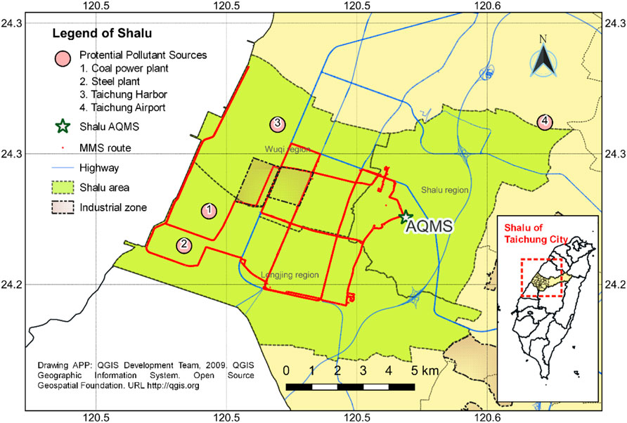
FIGURE 1. Location of Taichung City and the study area, Shalu.

PM_2.5 Monitoring Stations

On the north-western side of the Shalu area, one AQMS (latitude: 24.22563, longitude: 120.5688.) operated by the Taiwan EPA has been installed. In the present study, an MMS was established to collect concentrations of PM_2.5 at the ground level of different regions of the study area.

The Air Quality Monitoring Station

The AQMS is 15 m above the ground level with a sampling inlet at 19.5 m in height. The main monitoring items include fine suspended particulates (PM_2.5), coarse suspended particulates (PM₁₀), carbon monoxide (CO), sulfur dioxide (SO₂), ozone (O₃), nitrogen dioxide (NO₂), and meteorological data (UVB, rainfall, wind direction and wind speed, temperature, and humidity). The installed PM_2.5 monitoring instrument (model BAM-1020, Met One Instruments Inc., Grands Pass, OR) uses beta-rays for detecting the relative concentration of PM_2.5 (detection range: 0–10 mg/m³, resolution: 2 μg/m³, beta-ray source: C-14, filter paper: glass fiber, capture efficiency: 0.3 μm particulate matter> 99.999%, sampling flow rate: 16.7 LPM) once per hour automatically.

The Mobile Monitoring Station

An electric car (LUXGEN MPV EV+, battery module: lithium-ion) was chosen as a mobile platform for the MMS to avoid influences from vehicle self-emissions. The MMS is equipped with a DUSTTRAK II Aerosol Monitor (model 8,530, TSI Inc., St. Paul, MN, United States; detection range: 0.001–150 mg/m³, resolution: 1 μg/m³, sampling flow rate: 3 L/min, time resolution: one reading per second) to monitor PM_2.5 real-time concentrations and a GPS to record the latitude–longitude information. To prevent collected samples from being affected by road contaminants, the sampling inlet of the MMS is set at a height of 2.2 m and air samples are collected isokinetically. Table 1 shows the information on the station height, monitoring instrument, data collection frequency, and resolution for both the AQMS and MMS. Considering the intrinsic differences in the monitoring instruments of the AQMS and MMS, both the collected data (i.e., AQMS_m and MMS_m) were calibrated (i.e., AQMS_c and MMS_c) by reference to the Federal Reference Methods/Federal Equivalent Methods (FRM/FEM) (Environmental Protection Agency U.S, 2022).

TABLE 1

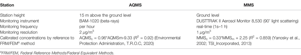
TABLE 1. Basic information for the AQMS and MMS used in the present study for measuring PM_2.5 concentrations.

Sampling Campaign

A sampling route ∼ 80 km in length was designed for the MMS to collect PM_2.5 concentrations in the study area. Samplings were conducted from September 2013 to August 2014 covering the four seasons. For each sampling day, samplings were conducted approximately from 6:00 to 17:00 and 18:00 to 23:00 during the daytime and nighttime, respectively. Details of the MMS and its QA/QC can be found in our previous work (Lin et al., 2018). To compare with AQMS-collected data (i.e., hourly data), all MMS-collected data were further processed as the hourly average values. All collected MMS data in the study area were classified into three regions as follows based on the obtained GPS records: the urban region, industrial region, and harbor region (Figure 2). Table 2 shows the details of the whole MMS sampling campaign. In the present study, the corresponding AQMS data were also recorded in accordance with the aforementioned MMS sampling campaign.

FIGURE 2

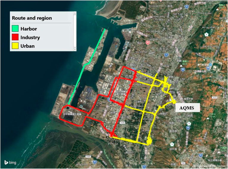
FIGURE 2. MMS sampling route in the three regions: urban (yellow), industrial (red), and harbor regions (green).

TABLE 2

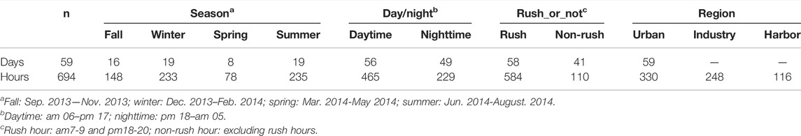
TABLE 2. Description of the whole MMS sampling campaign classified into the whole sampling days/hours by the season, day/night, rush/non-rush, and area.

Statistic Methods

Since the obtained PM_2.5 concentrations were lognormally distributed, logarithmic conversion was applied to both AQMS and MMS data. One-way ANOVA/paired t/t-tests were applied to examine the differences between the MMS and the AQMS in seasons, day/night, commute periods, and different areas.

To develop predicting models for establishing residents’ long-term PM_2.5 exposure concentrations at the ground level in different regions, MMS-measured data were compared with those obtained from the AQMS. Before the establishment of the aforementioned predicting models, possible interference factors were first identified, including three atmospheric variables [temperature (TEMP), relative humidity (RH), and wind speed (WS)], three primary pollutants (CO, NO_x, and SO₂), and one secondary pollutant (O₃) according to literature reviews (Cabada et al., 2004; Borge et al., 2016; Mazaheri et al., 2018; Adams et al., 2020; Liu et al., 2020). The hierarchical regression analysis was used to further confirm interference factors for the final predicting models. All data aggregation and statistics were performed using the Excel 365 software (Microsoft), R software (R x64 3.6.2) (R-Core-Team, 2019), and SPSS17 (IBM SPSS, 2008).

Conducting Health Impact Assessment

In the present study, ground-level PM_2.5 concentrations derived from predicting models were used for deriving the PM_2.5 mortality hazard ratio (HR) through the application of the GEMM as follows:

$\mathbf{HR}=\mathbf{GEMM}\left(\mathbf{z}\right)=\mathit{exp}\left[\mathbf{\theta }\text{∗}\mathbf{log}\left(\mathbf{z}/\mathbf{\alpha }+1\right)/\left(1+\mathit{exp}\left[-\left(\mathbf{z}-\mathbf{\mu }\right)/\mathbf{\nu }\right]\right)\right],(1)$

where z = max (0, C - C_rf), C = the exposed PM_2.5 concentration, and C_rf = the counterfactual PM_2.5 concentration (=2.4 μg/m³).

θ, SEθ, α, μ, and ν = parameters can be determined based on the cause of death (for the present study: lung cancer) by referring to Table 3.

TABLE 3

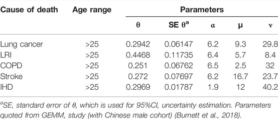
TABLE 3. Values for the parameter used in the GEMM.

Since the mortality probability of lung cancer is quite small, the resultant HR could serve as a surrogate for the relative risk (RR) (Burnett et al., 2018). The attributed fraction for the population (AF) of lung cancer can be calculated as follows (Ostro and WHO, 2004):

$\mathbf{AF}=\left(\mathbf{RR}-1\right)/\mathbf{RR}.(2)$

Results and Discussion

Comparisons of AQMS- and MMS-Measured PM_2.5 Concentrations

PM_2.5 concentrations of the whole sampling year, seasonal, diurnal, and rush/non-rush hour obtained from both the AQMS and MMS are compared and shown in Table 4. From the whole sampling year aspect, MMS results (GM = 25.9 μg/m³; 95% CI = 24.8–27.1 μg/m³) are significantly higher than those of the AQMS (GM = 23.3 μg/m³; 95% CI = 22.3–24.3 μg/m³) (t-test; p < 0.01). The former is 1.23 times (95% CI = 1.18-1.27) higher in magnitude than the latter. The aforementioned result is not so surprising since the MMS was much closer to PM_2.5 emission sources (such as traffic) than the AQMS (Wu et al., 2014). In addition, our results are also consistent with previous studies. For example, a study conducted in Boston’s Chinatown (near a highway) shows that the increase of building elevation from 0 to 35 m would result in a decrease of the PM_2.5 mass concentration by 5.1% (Wu et al., 2014). Another study conducted in Pittsburgh, Pennsylvania, shows that the annual MMS is higher than the annual average of the AQMS (14.6 and 10.2 μg/m³, respectively) (Li et al., 2016). Here, it should be noted that the latter study was simply conducted in the 2013 winter and 2014 summer (i.e., does not cover four seasons), and hence no statistical significance could be found.

TABLE 4

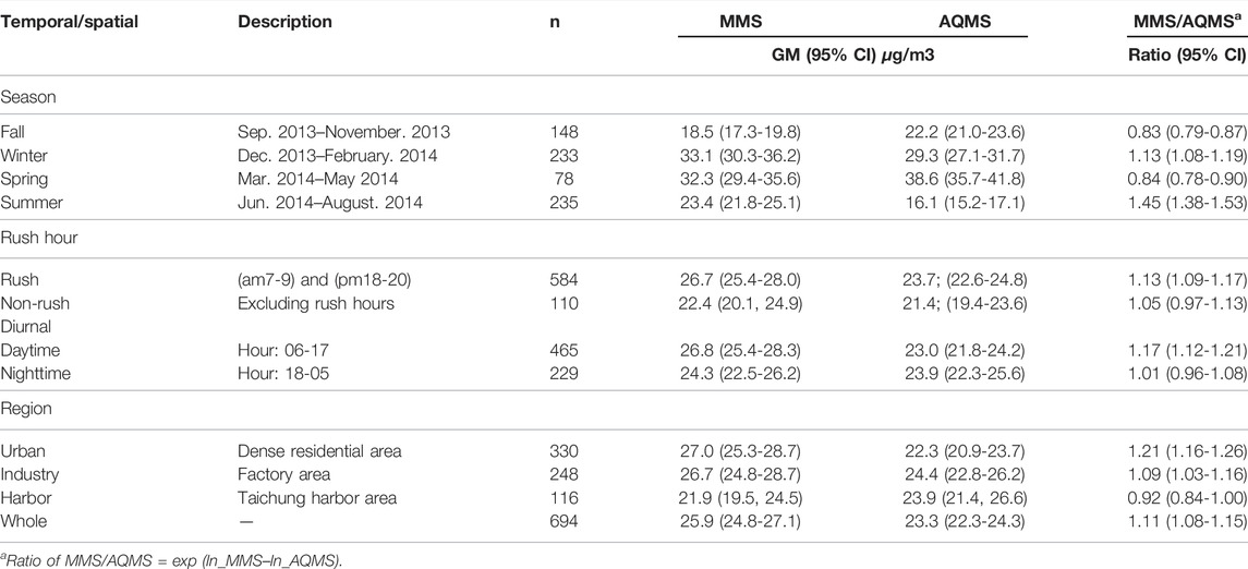
TABLE 4. Comparison of PM_2.5 concentrations of the whole sampling year, seasonal, diurnal, and rush/non-rush hour for data obtained from both the AQMS and MMS.

For seasonal PM_2.5 mass concentrations, MMS results are statistically significantly higher than those of the AQMS in both summer (GM = 23.4 and 16.1 μg/m³, 95% CI = 21.8–25.1 and 15.2–17.1 μg/m³, respectively; paired t-test; p < 0.001) and winter (GM = 33.1 and 29.3 μg/m³, 95% CI = 30.3–36.2 and 27.1–31.7 μg/m³, respectively; paired t-test; p < 0.001). However, an opposite trend is found in both spring (GM = 32.3 and 38.6 μg/m³, 95% CI = 29.4–35.6 and 35.7–41.8 μg/m³, respectively; paired t-test; p < 0.001) and fall (GM = 18.5 and 22.3 μg/m³, 95% CI = 17.3–19.8 and 21.0, 23.6 μg/m³, respectively; paired t-test; p < 0.001). The opposite trend found in spring and fall might be associated with the lower atmospheric boundary layer, and more significant temperature inversions were found in these two seasons (Ye et al., 2018; Yousefian et al., 2020).

Since the MMS was more proximal to traffic PM_2.5 emission sources than the AQMS, as expected, we found that the MMS rush hour results (GM = 26.7 μg/m³, 95% CI: 25.4–28.0 μg/m³) are significantly higher than those of the AQMS (GM = 23.7 μg/m³, 95% CI = 22.6–24.8 μg/m³) (paired sample t-test; p < 0.001). Although the same trend can also be found for data collected during non-rush hours, however, no statistical significance is found in the present study (GM = 22.4 and 21.4 μg/m³, 95% CI = 20.1–24.9 and 19.4–23.6 μg/m³ for the MMS and AQMS, respectively; paired t-test; p = 0.234). Obviously, the aforementioned result could be due to less traffic density during non-rush hours. The aforementioned reason can also be used to explain the diurnal sampling results. Here, the daytime sampling results show that those of the MMS are significantly higher than those of the AQMS (GM = 26.8 and 23.0 μg/m³, 95% CI = 25.4–28.3 and 21.8–24.2 μg/m³, respectively; paired t-test; p < 0.001)). Although nighttime sampling results for the MMS are higher than those of the AQMS, no statistical significance is found in the present study (GM = 24.3 and 23.9 μg/m³, 95% CI = 22.5–26.2 and 22.3–25.6 μg/m³, respectively; paired t-test; p = 0.635).

Comparisons of PM_2.5 Concentrations of the Urban, Industry, and Harbor Regions Obtained From the MMS and Those Simultaneously Obtained From the AQMS

Table 4 shows the PM_2.5 concentrations of the urban, industry, and harbor regions, and the whole Shalu area data obtained from the MMS. No significant difference (ANOVA post hoc test, p =0.978) could be found between PM_2.5 concentrations of the urban region (GM = 27.0 μg/m³, 95% CI = 25.3–28.7 μg/m³) and industry region (GM = 26.7 μg/m³, 95% CI = 24.8–28.7 μg/m³). Considering that the dimension of the whole Shalu area is less than 100 km², the geographical adjacency of both regions might lead to a similarity in their PM_2.5 concentrations. On the other hand, both PM_2.5 concentrations of the aforementioned two regions were significantly higher than those of the harbor region (GM = 21.9 μg/m³, 95% CI = 19.5–24.5 μg/m³) ug/m³ (ANOVA post hoc test; p < 0.01). It could be due to fewer ground-level pollution sources in the harbor region than that in others. In addition, its remote location from the other two regions and the effect of the monsoon wind direction could also be considered contributors (Cheng and Hsu, 2019).

For the comparison purpose, PM_2.5 concentrations of the urban, industry, and harbor regions obtained from the MMS were compared with those simultaneously obtained from the AQMS. For both urban and industrial regions, the MMS concentration (GM = 27.0 and 26.7 μg/m³, 95% CI = 25.3-28.7 and 24.8–28.7 μg/m³, respectively) is significantly higher than that of the AQMS (GM = 22.3 and 24.4 μg/m³, 95% CI = 20.9-23.7 and 22.8–26.2 μg/m³, respectively) (paired t-test; p < 0.001). For the harbor region, however, the MMS concentration (GM = 21.9 μg/m³, 95% CI = 19.5–24.5 μg/m³) is significantly less than that of the AQMS (GM = 23.9 μg/m³, 95% CI = 21.4–26.6 μg/m³) (paired t-test; p =0.046). The aforementioned results might be because of the existence of fewer ground-level pollution sources in the harbor region. For both urban and industrial regions, the PM_2.5 concentration of the MMS is respectively 1.21 and 1.09 times higher in magnitude than that of the AQMS. The aforementioned results might be because the urban region is proximal to traffic pollution sources, and the industrial region is mainly affected by pollution sources associated with manufacturing and heavy truck emission.

Establishing the Relationship Between PM_2.5 Concentrations of the AQMS and MMS

Multivariate linear regression (MLR) analyses (hierarchical regression) were conducted to identify variables used for establishing predicting models through examining the variability and collinearity of candidate interference factors. The statistical significance can be found for the four factors, CO, SO₂, WS, and AQMS PM_2.5 concentrations. The aforementioned four factors were first included for establishing predicting models (R² = 0.58). Considering that the total contribution of SO₂, CO, and WS to R² is less than 7%, they were removed from the prediction models pragmatically for practical reasons (see Supplementary Table S1). The ignorance of the aforementioned factors is consistent with previous studies conducted in Lubbock, Texas (Kelley et al., 2020), Tianjin, Beijing, and Hebei provinces in China (Zhang et al., 2018). Considering the intrinsic difference in PM_2.5 concentrations of the urban, industrial, and harbor regions, predicting models were established not only based on the data collected from the whole area but also each individual region. The resultant predicting models are shown as follows:

Whole area:

$\mathrm{ln\_MMS}=0.839\mathrm{+}0.768\ast \mathrm{ln\_AQMS,}\left(\mathrm{RMSE}=1.50\mathit{\mu g}/{\mathrm{m}}^{\mathrm{3}}\mathrm{,}{\mathrm{R}}^{\mathrm{2}}\mathrm{=}0.54\mathrm{; n}\mathrm{=694}\right).\left(3\right)$

Urban region:

$\mathrm{ln\_MMS}=0.691\mathrm{+}0.839\ast \mathrm{ln\_AQMS,}\left(\mathrm{RMSE}=1.42\mathit{\mu g}/{\mathrm{m}}^{\mathrm{3}}\mathrm{,}{\mathrm{R}}^{\mathrm{2}}\mathrm{=}0.65\mathrm{; n}\mathrm{=330}\right).\left(4\right)$

Industrial region:

$\mathrm{ln\_MMS}=1.037\mathrm{+}0.703\ast \mathrm{ln\_AQMS,}\left(\mathrm{RMSE}=1.55\mathit{\mu g}/{\mathrm{m}}^{\mathrm{3}}\mathrm{,}{\mathrm{R}}^{\mathrm{2}}\mathrm{=}0.45\mathrm{; n}\mathrm{=248}\right).\left(5\right)$

Harbor region:

$\mathrm{ln\_MMS}=0.714\mathrm{+}0.747\ast \mathrm{ln\_AQMS,}\left(\mathrm{RMSE}=1.55\mathit{\mu g}/{\mathrm{m}}^{\mathrm{3}}\mathrm{,}{\mathrm{R}}^{\mathrm{2}}\mathrm{=}0.51\mathrm{; n}\mathrm{=116}\right).\left(6\right)$

Figures 3A–D show the scatter plots of the MMS and AQMS for data collected from the whole study area, urban, industrial, and harbor regions, respectively. The R² obtained from the present study is comparable with another study for predicting outdoor personal exposures using nearby AQMS PM_2.5 concentrations (Miller et al., 2019). In the present study, the ANOVA (post hoc test) was performed to examine if there is a statistical significance among the four predicting models (See Supplementary Table S2). Results show that no significant difference can be found among the three predicting models for the whole area, urban region, and industrial region; however, the slope of the predicting model for the harbor region was significantly lower than that of others (all p < 0.05). The aforementioned results are consistent with a study conducted in Guangzhou, China, where the relationship between AQMS PM_2.5 concentrations and personal exposure varies greatly from district to district (Jahn et al., 2013). Here, it should be noted that it would be more reasonable to have one predicting model for both urban and industrial regions from a statistical point of view. However, considering the intrinsic difference in the emission sources of the aforementioned two regions, using two separate predicting models could be feasible to meet practical purposes. In the present study, the established four predicting models were adopted for predicting the residents’ exposures and further for conducting health impact analyses of each individual region and the whole area.

FIGURE 3

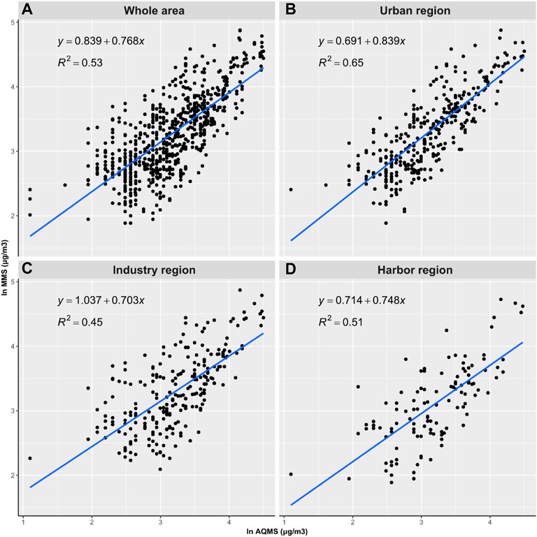
FIGURE 3. Scatter plots of the MMS and AQMS for the (A) whole area, (B) urban region, (C) industry region, and (D) harbor region.

Health Impact Assessment for Each Individual Region and the Whole Area

Seven-year (2013–2019) AQMS-measured concentrations (i.e., AQMS_7-yr) were used to establish the long-term PM_2.5 concentrations at the ground level (i.e., MMS_7-yr) of the whole area and the three different regions using Eqs 3–6, respectively (Table 5). Health impact functions and local health data were used to quantify the PM_2.5-attributable health burden for both AQMS_7-yr and MMS_7-yr, respectively. The above ground-level PM_2.5 concentrations together with the parameter values shown in Table 3 for lung cancer were applied to the GEMM (Eq. 1) for deriving the PM_2.5 mortality hazard ratio (HR). Since the mortality probability of lung cancer is small, the HR obtained from the present study was used as a surrogate for the relative risk (RR) (Burnett et al., 2018). Table 5 also shows the lung cancer-attributed fraction (AF) of the population using Eq. 2. Results show that both AQMS_7-yr and MMS_7-yr decreased from 2013–2019, and the former is lower than the latter. As a result, the same downward trend can also be seen in the estimated RR and AF over the years.

TABLE 5

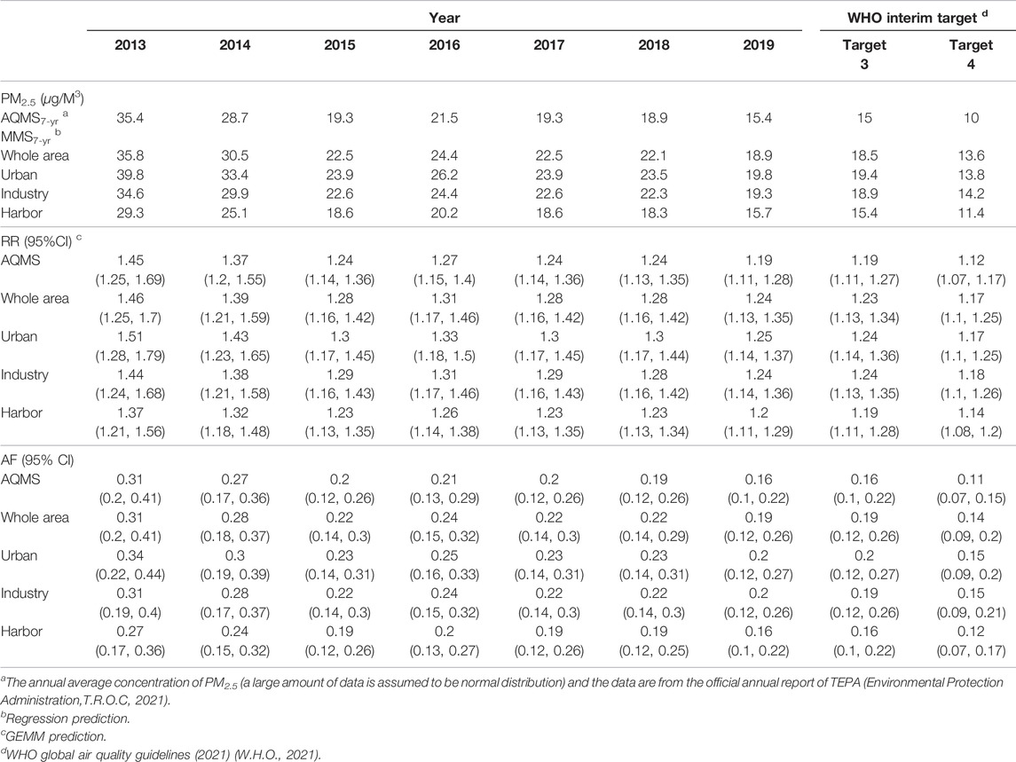
TABLE 5. Annual mean of PM_2.5 concentrations of AQMS_7-yr and the ground level (MMS7-yr) of the whole Shalu area and their derived relative risks (RRs) and the attributed fraction of the population (AF).

For the whole area, AQMS PM_2.5 concentrations from 2013–2019 are, in total, decreased by 56% (i.e., from 35.4 to 15.4 μg/m³), the resultant decrease for the RR was 20% (i.e., from 1.45 to 1.19) and AF was 48% (i.e., from 0.31 to 0.16). Therefore, reducing the AQMS PM_2.5 concentrations (i.e., AQMS_7-yr) has a high contribution to the lung cancer AF. Here, it should be noted that even if the yearly average AQMS PM_2.5 concentration meets the government and WHO PM_2.5 interim targets 3 and 4 (i.e., 15 and 10 μg/m3, respectively) (W.H.O., 2021), the resultant AFs still cannot be ignored (= 16 and 11%, respectively). Similar results can also be seen in MMS_7-yr [i.e., PM_2.5 concentrations decreased by 47% in total (i.e., from 35.8 to 18.9 μg/m³), RR by 15% (i.e., from 1.46 to 1.24), and AF by 39% (i.e., from 0.31 to 0.19)]. Even if the yearly average AQMS PM_2.5 concentration meets the government and WHO PM_2.5 interim targets 3 and 4, the estimated MMS_7-y (i.e., 18.5 and 13.6, respectively) would lead to even higher AFs (=19 and 14%, respectively) in comparison with the corresponding values (= 16 and 11%, respectively) associated with AQMS PM_2.5 concentrations.

Table 5 also shows the estimated annual mean of PM_2.5 concentrations at the ground level (MMS_7-yr) of the urban, industrial, and harbor regions, and the corresponding attributed fraction of the population (AF) for lung cancer. The trend in the decrease of PM_2.5 concentrations from 2013 to 2019 and the decrease in the resultant RR are similar to those found in the whole area. Moreover, it can also be seen that if AQMS_7-yr is used for estimating the AF for residents in the Shalu area, an average underestimation of 10.4% was yielded in comparison with those using MMS_7-yr. The decrease of unit PM_2.5 concentration would lead to the decrease in the AF of lung cancer by 0.75 and 0.71% in AQMS_7-yr and MMS_7-yr, respectively. By applying Eq. 3 to the whole Taiwan area, directly using AQMS_7-yr would lead to an underestimation of ∼ 1,000 lung cancer deaths annually in Taiwan during the period from 2013 to 2019 in comparison with those using MMS_7-yr (See Supplementary Figure S3). The aforementioned results further strengthen the importance of developing methodologies for predicting PM_2.5 concentrations at the ground level.

Limitations and Future Implications

Considering that there were annual increases in the number of residents, vehicles, and manufacturing industries from 2014 to 2019, it would be more reasonable to establish predicting models based on data collected from the same period of time. In the present study, although before the establishment of the predicting models, possible interference factors were identified (including atmospheric variables, primary pollutants, and secondary pollutants), which would lead to the developed predicting models becoming more suitable for complicated pollution scenarios. Nevertheless, the establishment of the prediction model in the present study is simply based on data collected from 2013 to 2014 for practical reasons. The aforementioned factor should be considered a limitation of the present study. Moreover, possible interference factors in the present study were considered as those affecting PM_2.5 concentrations. The selection of possible interference factors was based on the results of literature reviews and available information collected by the AQMS. Indeed, some VOCs are known to be associated with the formation of secondary aerosols, which will also affect the concentrations of PM_2.5. However, considering no VOC information could be obtained from the AQMS, only three atmospheric variables, three primary pollutants, and one secondary pollutant were selected. The aforementioned deficiency might explain the R² of the predicting models falling to the range 0.45–0.65. We believe that the addition of some VOCs might increase the magnitude of R² of the predicting models. The aforementioned factor can also be considered a limitation of the present study.

This study was set out to develop an integrated approach for effectively predicting PM_2.5 exposures for residents at the ground level via the combination of the concentrations measured across different seasons and regions using the MMS and those obtained from the nearby fixed-site AQMS. Our results strongly suggest that using the ground-level concentrations would be more accurate in assessing residents’ health impacts than those directly obtained from the AQMS. Since the AQMS has been intensively installed in many countries, AQMS data have been widely used for pollution alerts for residents, policy-making for pollution control strategies, and global disease burden assessment. Therefore, the methodology developed from the present study would provide us with a feasible approach for predicting the ground-level concentrations which will effectively enhance the value of the AQMS installed in many countries. Moreover, the approach developed from the present study will be also beneficial to the epidemiological research field for better assessing health outcomes associated with residents’ PM_2.5 exposures.

Conclusion

In this study, we presented a methodology for assessing the PM_2.5 exposures of residents and their health impacts at a city level. We found that there is a significant linear relationship between MMS-measured ground-level concentrations and the corresponding concentrations obtained from the AQMS of the area, and the former is higher than that of the latter. A consistent trend in PM_2.5 exposures associated with the spatial difference was found as industry region $\cong$ urban region > harbor region. Our results clearly indicate that residents’ ambient PM_2.5 exposures do exist with spatial differences in both vertical and horizontal spaces. The health impact assessment results show that the use of AQMS data would lead to an underestimation of ∼ 10.4% in magnitude in the estimated lung cancer death attributed fraction (AF) in comparison with those using ground-level exposure concentrations. Similarly, directly using the former would lead to an underestimation of ∼ 1,000 lung cancer deaths annually in Taiwan during the period from 2013 to 2019, in comparison with those using the latter. The present study clearly indicates the importance of developing methodologies for predicting residents’ ground-level PM_2.5 exposure concentrations in conducting exposure and health impact assessments.

Data Availability Statement

The raw data supporting the conclusions of this article will be made available by the authors, without undue reservation.

Author Contributions

Study design: P-JT and M-YL. Field data collection: M-SH, M-YL, L-HY, H-TH. Statistical analyses: M-SH, B-FH, and J-DW. Manuscript preparation: M-SH and P-JT.

Conflict of Interest

The authors declare that the research was conducted in the absence of any commercial or financial relationships that could be construed as a potential conflict of interest.

Publisher’s Note

All claims expressed in this article are solely those of the authors and do not necessarily represent those of their affiliated organizations, or those of the publisher, the editors, and the reviewers. Any product that may be evaluated in this article, or claim that may be made by its manufacturer, is not guaranteed or endorsed by the publisher.

Acknowledgments

The authors would like to thank the National Health Research Institute in Taiwan for funding this research project. The author M-YL has the same contribution to this research project as the corresponding author.

Supplementary Material

The Supplementary Material for this article can be found online at: https://www.frontiersin.org/articles/10.3389/fenvs.2022.901754/full#supplementary-material

References

Adams, M. D., Massey, F., Chastko, K., and Cupini, C. (2020). Spatial Modelling of Particulate Matter Air Pollution Sensor Measurements Collected by Community Scientists while Cycling, Land Use Regression with Spatial Cross-Validation, and Applications of Machine Learning for Data Correction. Atmos. Environ. 230, 10. doi:10.1016/j.atmosenv.2020.117479

CrossRef Full Text | Google Scholar

Borge, R., Narros, A., Artíñano, B., Yagüe, C., Gómez-Moreno, F. J., De La Paz, D., et al. (2016). Assessment of Microscale Spatio-Temporal Variation of Air Pollution at an Urban Hotspot in Madrid (Spain) through an Extensive Field Campaign. Atmos. Environ. 140, 432–445. doi:10.1016/j.atmosenv.2016.06.020

CrossRef Full Text | Google Scholar

Burnett, R., Chen, H., Szyszkowicz, M., Fann, N., Hubbell, B., Pope, C. A., et al. (2018). Global Estimates of Mortality Associated with Long-Term Exposure to Outdoor Fine Particulate Matter. Proc. Natl. Acad. Sci. U.S.A. 115, 9592–9597. doi:10.1073/pnas.1803222115

PubMed Abstract | CrossRef Full Text | Google Scholar

Cabada, J. C., Khlystov, A., Wittig, A. E., Pilinis, C., and Pandis, S. N. (2004). Light Scattering by Fine Particles during the Pittsburgh Air Quality Study: Measurements and Modeling. J. Geophys. Res.-Atmos. 109 (D16), 1–13. doi:10.1029/2003jd004155

CrossRef Full Text | Google Scholar

Caplin, A., Ghandehari, M., Lim, C., Glimcher, P., and Thurston, G. (2019). Advancing Environmental Exposure Assessment Science to Benefit Society. Nat. Commun. 10, 1236. doi:10.1038/s41467-019-09155-4

PubMed Abstract | CrossRef Full Text | Google Scholar

Castell, N., Dauge, F. R., Schneider, P., Vogt, M., Lerner, U., Fishbain, B., et al. (2017). Can Commercial Low-Cost Sensor Platforms Contribute to Air Quality Monitoring and Exposure Estimates? Environ. Int. 99, 293–302. doi:10.1016/j.envint.2016.12.007

PubMed Abstract | CrossRef Full Text | Google Scholar

Chen, P., Bi, X., Zhang, J., Wu, J., and Feng, Y. (2015). Assessment of Heavy Metal Pollution Characteristics and Human Health Risk of Exposure to Ambient PM2.5 in Tianjin, China. Particuology 20, 104–109. doi:10.1016/j.partic.2014.04.020

CrossRef Full Text | Google Scholar

Cheng, F.-Y., and Hsu, C.-H. (2019). Long-Term Variations in PM2.5 Concentrations under Changing Meteorological Conditions in Taiwan. Sci. Rep. 9, 6635. doi:10.1038/s41598-019-43104-x

PubMed Abstract | CrossRef Full Text | Google Scholar

Cheng, Y.-H., Ninh, X.-H., and Yeh, S.-L. (2019). Dominant Factors Influencing the Concentrations of Particulate Matters inside Train Carriages Traveling in Different Environments in the Taipei Mass Rapid Transit System. Aerosol Air Qual. Res. 19, 1579–1592. doi:10.4209/aaqr.2018.09.0335

CrossRef Full Text | Google Scholar

Dias, D., and Tchepel, O. (2018). Spatial and Temporal Dynamics in Air Pollution Exposure Assessment. Int. J. Environ. Res. Public Health 15, 558. doi:10.3390/ijerph15030558

PubMed Abstract | CrossRef Full Text | Google Scholar

Dröge, J., Müller, R., Scutaru, C., Braun, M., and Groneberg, D. (2018). Mobile Measurements of Particulate Matter in a Car Cabin: Local Variations, Contrasting Data from Mobile versus Stationary Measurements and the Effect of an Opened versus a Closed Window. Ijerph 15, 2642. doi:10.3390/ijerph15122642

CrossRef Full Text | Google Scholar

Environmental Protection Administration, T.R.O.C (2020). Manual Monitoring of Fine Fine Suspended Particles [Online]. Taipei Taiwan. Available at: https://airtw.epa.gov.tw/CHT/EnvMonitoring/Central/spm.aspx (Accessed May 5, 2019).

Google Scholar

Environmental Protection Administration, T.R.O.C (2021). Yearly Reports of Air Monitoring [Online]. Teipei, Taiwan: EPA. Available at: https://www.epa.gov.tw/Page/672FA2BDDEAA22C7/71fedbd8-9829-49e0-b02b-0addb5bd470a?msclkid=1aaa7477a97811ec8a50451d458a7bb7 (Accessed Mar 5, 2020).

Google Scholar

Environmental Protection Agency U.S. (2021). Air Sensor Toolbox [Online]. EPA. Available at: https://www.epa.gov/air-sensor-toolbox (Accessed Mar 2, 2021).

Google Scholar

Environmental Protection Agency U.S. (2022). EPA Scientists Develop and Evaluate Federal Reference & Equivalent Methods for Measuring Key Air Pollutants [Online]. EPA. Available at: https://www.epa.gov/air-research/epa-scientists-develop-and-evaluate-federal-reference-equivalent-methods-measuring-key (Accessed Sep 1, 2019).

Google Scholar

Environmental Protection Agency U.S. (2019). Integrated Science Assessment (ISA) for Particulate Matter. Washington, DC: U.S. Environmental Protection Agency. (Final Report, Dec 2019).

Google Scholar

Fishbain, B., Lerner, U., Castell, N., Cole-Hunter, T., Popoola, O., Broday, D. M., et al. (2017). An Evaluation Tool Kit of Air Quality Micro-sensing Units. Sci. Total Environ. 575, 639–648. doi:10.1016/j.scitotenv.2016.09.061

PubMed Abstract | CrossRef Full Text | Google Scholar

Forouzanfar, M. H., Afshin, A., Alexander, L. T., Anderson, H. R., Bhutta, Z. A., Biryukov, S., et al. (2016). Global, Regional, and National Comparative Risk Assessment of 79 Behavioural, Environmental and Occupational, and Metabolic Risks or Clusters of Risks, 1990-2015: a Systematic Analysis for the Global Burden of Disease Study 2015. Lancet 388, 1659–1724. doi:10.1016/S0140-6736(16)31679-8

PubMed Abstract | CrossRef Full Text | Google Scholar

Fuller, R., Sandilya, K., and Hanrahan, D. (2019). Pollution and Health Metrics: Global, Regional and Country Analysis. GAHP, Global Alliance on Health and Pollution.

Google Scholar

Guo, H., Gu, X., Ma, G., Shi, S., Wang, W., Zuo, X., et al. (2019). Spatial and Temporal Variations of Air Quality and Six Air Pollutants in China during 2015-2017. Sci. Rep. 9, 15201. doi:10.1038/s41598-019-50655-6

PubMed Abstract | CrossRef Full Text | Google Scholar

Han, X., and Naeher, L. P. (2006). A Review of Traffic-Related Air Pollution Exposure Assessment Studies in the Developing World. Environ. Int. 32, 106–120. doi:10.1016/j.envint.2005.05.020

PubMed Abstract | CrossRef Full Text | Google Scholar

Hankey, S., and Marshall, J. D. (2015). On-bicycle Exposure to Particulate Air Pollution: Particle Number, Black Carbon, PM 2.5 , and Particle Size. Atmos. Environ. 122, 65–73. doi:10.1016/j.atmosenv.2015.09.025

CrossRef Full Text | Google Scholar

Hu, L., Liu, J., and He, Z. (2016). Self-Adaptive Revised Land Use Regression Models for Estimating PM2.5 Concentrations in Beijing, China. Sustainability 8, 786. doi:10.3390/su8080786

CrossRef Full Text | Google Scholar

Jahn, H. J., Kraemer, A., Chen, X.-C., Chan, C.-Y., Engling, G., and Ward, T. J. (2013). Ambient and Personal PM2.5 Exposure Assessment in the Chinese Megacity of Guangzhou. Atmos. Environ. 74, 402–411. doi:10.1016/j.atmosenv.2013.04.011

CrossRef Full Text | Google Scholar

Jeong, C.-H., Wang, J. M., Hilker, N., Debosz, J., Sofowote, U., Su, Y., et al. (2019). Temporal and Spatial Variability of Traffic-Related PM2.5 Sources: Comparison of Exhaust and Non-exhaust Emissions. Atmos. Environ. 198, 55–69. doi:10.1016/j.atmosenv.2018.10.038

CrossRef Full Text | Google Scholar

Jung, C.-R., Hwang, B.-F., and Chen, W.-T. (2018). Incorporating Long-Term Satellite-Based Aerosol Optical Depth, Localized Land Use Data, and Meteorological Variables to Estimate Ground-Level PM2.5 Concentrations in Taiwan from 2005 to 2015. Environ. Pollut. 237, 1000–1010. doi:10.1016/j.envpol.2017.11.016

PubMed Abstract | CrossRef Full Text | Google Scholar

Kelley, M. C., Brown, M. M., Fedler, C. B., and Ardon-Dryer, K. (2020). Long-term Measurements of PM2.5 Concentrations in Lubbock, Texas. Aerosol Air Qual. Res. 20, 1306–1318. doi:10.4209/aaqr.2019.09.0469

CrossRef Full Text | Google Scholar

Kingham, S., Longley, I., Salmond, J., Pattinson, W., and Shrestha, K. (2013). Variations in Exposure to Traffic Pollution while Travelling by Different Modes in a Low Density, Less Congested City. Environ. Pollut. 181, 211–218. doi:10.1016/j.envpol.2013.06.030

PubMed Abstract | CrossRef Full Text | Google Scholar

Kuo, P.-H., Tsuang, B.-J., Chen, C.-J., Hu, S.-W., Chiang, C.-J., Tsai, J.-L., et al. (2014). Risk Assessment of Mortality for All-Cause, Ischemic Heart Disease, Cardiopulmonary Disease, and Lung Cancer Due to the Operation of the World's Largest Coal-Fired Power Plant. Atmos. Environ. 96, 117–124. doi:10.1016/j.atmosenv.2014.07.024

CrossRef Full Text | Google Scholar

Lee, C.-H., Wang, Y.-B., and Yu, H.-L. (2019). An Efficient Spatiotemporal Data Calibration Approach for the Low-Cost PM2.5 Sensing Network: A Case Study in Taiwan. Environ. Int. 130, 104838. doi:10.1016/j.envint.2019.05.032

PubMed Abstract | CrossRef Full Text | Google Scholar

Lee, M., Lin, L., Chen, C.-Y., Tsao, Y., Yao, T.-H., Fei, M.-H., et al. (2020). Forecasting Air Quality in Taiwan by Using Machine Learning. Sci. Rep. 10, 4153. doi:10.1038/s41598-020-61151-7

PubMed Abstract | CrossRef Full Text | Google Scholar

Li, H. Z., Dallmann, T. R., Gu, P., and Presto, A. A. (2016). Application of Mobile Sampling to Investigate Spatial Variation in Fine Particle Composition. Atmos. Environ. 142, 71–82. doi:10.1016/j.atmosenv.2016.07.042

CrossRef Full Text | Google Scholar

Li, J., Mattewal, S. K., Patel, S., and Biswas, P. (2020). Evaluation of Nine Low-Cost-Sensor-Based Particulate Matter Monitors. Aerosol Air Qual. Res. 20, 254–270. doi:10.4209/aaqr.2018.12.0485

CrossRef Full Text | Google Scholar

Li, Z., Fung, J. C. H., and Lau, A. K. H. (2018). High Spatiotemporal Characterization of On-Road PM2.5 Concentrations in High-Density Urban Areas Using Mobile Monitoring. Build. Environ. 143, 196–205. doi:10.1016/j.buildenv.2018.07.014

CrossRef Full Text | Google Scholar

Lin, M.-Y., Guo, Y.-X., Chen, Y.-C., Chen, W.-T., Young, L.-H., Lee, K.-J., et al. (2018). An Instantaneous Spatiotemporal Model for Predicting Traffic-Related Ultrafine Particle Concentration through Mobile Noise Measurements. Sci. Total Environ. 636, 1139–1148. doi:10.1016/j.scitotenv.2018.04.248

PubMed Abstract | CrossRef Full Text | Google Scholar

Lin, Y.-C., Chi, W.-J., and Lin, Y.-Q. (2020). The Improvement of Spatial-Temporal Resolution of PM2.5 Estimation Based on Micro-Air Quality Sensors by Using Data Fusion Technique. Environ. Int. 134, 105305. doi:10.1016/j.envint.2019.105305

PubMed Abstract | CrossRef Full Text | Google Scholar

Liu, X., Schnelle-Kreis, J., Zhang, X., Bendl, J., Khedr, M., Jakobi, G., et al. (2020). Integration of Air Pollution Data Collected by Mobile Measurement to Derive a Preliminary Spatiotemporal Air Pollution Profile from Two Neighboring German-Czech Border Villages. Sci. Total Environ. 722, 137632. doi:10.1016/j.scitotenv.2020.137632

PubMed Abstract | CrossRef Full Text | Google Scholar

Maji, K. J., Arora, M., and Dikshit, A. K. (2017). Burden of Disease Attributed to Ambient PM2.5 and PM10 Exposure in 190 Cities in China. Environ. Sci. Pollut. Res. 24, 11559–11572. doi:10.1007/s11356-017-8575-7

PubMed Abstract | CrossRef Full Text | Google Scholar

Malings, C., Tanzer, R., Hauryliuk, A., Saha, P. K., Robinson, A. L., Presto, A. A., et al. (2020). Fine Particle Mass Monitoring with Low-Cost Sensors: Corrections and Long-Term Performance Evaluation. Aerosol Sci. Technol. 54, 160–174. doi:10.1080/02786826.2019.1623863

CrossRef Full Text | Google Scholar

Malmqvist, E., Lisberg Jensen, E., Westerberg, K., Stroh, E., Rittner, R., Gustafsson, S., et al. (2018). Estimated Health Benefits of Exhaust Free Transport in the City of Malmö, Southern Sweden. Environ. Int. 118, 78–85. doi:10.1016/j.envint.2018.05.035

PubMed Abstract | CrossRef Full Text | Google Scholar

Mazaheri, M., Clifford, S., Yeganeh, B., Viana, M., Rizza, V., Flament, R., et al. (2018). Investigations into Factors Affecting Personal Exposure to Particles in Urban Microenvironments Using Low-Cost Sensors. Environ. Int. 120, 496–504. doi:10.1016/j.envint.2018.08.033

PubMed Abstract | CrossRef Full Text | Google Scholar

Miller, K. A., Spalt, E. W., Gassett, A. J., Curl, C. L., Larson, T. V., Avol, E., et al. (2019). Estimating Ambient-Origin PM2.5 Exposure for Epidemiology: Observations, Prediction, and Validation Using Personal Sampling in the Multi-Ethnic Study of Atherosclerosis. J. Expo. Sci. Environ. Epidemiol. 29, 227–237. doi:10.1038/s41370-018-0053-x

PubMed Abstract | CrossRef Full Text | Google Scholar

Monrad, M., Sajadieh, A., Christensen, J. S., Ketzel, M., Raaschou-Nielsen, O., Tjønneland, A., et al. (2017). Long-Term Exposure to Traffic-Related Air Pollution and Risk of Incident Atrial Fibrillation: A Cohort Study. Environ. Health Perspect. 125, 422–427. doi:10.1289/ehp392

PubMed Abstract | CrossRef Full Text | Google Scholar

Morawska, L., Thai, P. K., Liu, X., Asumadu-Sakyi, A., Ayoko, G., Bartonova, A., et al. (2018). Applications of Low-Cost Sensing Technologies for Air Quality Monitoring and Exposure Assessment: How Far Have They Gone? Environ. Int. 116, 286–299. doi:10.1016/j.envint.2018.04.018

PubMed Abstract | CrossRef Full Text | Google Scholar

Mustafic, H., Jabre, P., Caussin, C., Murad, M. H., Escolano, S., Tafflet, M., et al. (2012). Main Air Pollutants and Myocardial Infarction: a Systematic Review and Meta-Analysis. JAMA 307, 713–721. doi:10.1001/jama.2012.126

PubMed Abstract | CrossRef Full Text | Google Scholar

Okokon, E. O., Yli-Tuomi, T., Turunen, A. W., Taimisto, P., Pennanen, A., Vouitsis, I., et al. (2017). Particulates and Noise Exposure during Bicycle, Bus and Car Commuting: A Study in Three European Cities. Environ. Res. 154, 181–189. doi:10.1016/j.envres.2016.12.012

PubMed Abstract | CrossRef Full Text | Google Scholar

Ostro, B.WHO (2004). Outdoor Air Pollution: Assessing the Environmental Burden of Disease at National and Local Levels. Geneva: World Health Organization.

Google Scholar

Özkaynak, H., Baxter, L. K., Dionisio, K. L., and Burke, J. (2013). Air Pollution Exposure Prediction Approaches Used in Air Pollution Epidemiology Studies. J. Expo. Sci. Environ. Epidemiol. 23, 566–572. doi:10.1038/jes.2013.15

PubMed Abstract | CrossRef Full Text | Google Scholar

Piotrowicz, A., and Polednik, B. (2019). Exposure to Aerosols Particles on an Urban Road. J. Ecol. Eng. 20, 27–34. doi:10.12911/22998993/105329

CrossRef Full Text | Google Scholar

R-Core-Team (2019). R: A Language and Environment for Statistical Computing. 2 ed. Vienna: R Foundation for Statistical Computing. R x64 3.6.

Google Scholar

Rittner, R., Gustafsson, S., Spanne, M., and Malmqvist, E. (2020). Particle Concentrations, Dispersion Modelling and Evaluation in Southern Sweden. Sn Appl. Sci. 2, 15. doi:10.1007/s42452-020-2769-1

CrossRef Full Text | Google Scholar

Saraswat, A., Apte, J. S., Kandlikar, M., Brauer, M., Henderson, S. B., and Marshall, J. D. (2013). Spatiotemporal Land Use Regression Models of Fine, Ultrafine, and Black Carbon Particulate Matter in New Delhi, India. Environ. Sci. Technol. 47, 12903–12911. doi:10.1021/es401489h

PubMed Abstract | CrossRef Full Text | Google Scholar

Shen, J., and Gao, Z. (2019). Commuter Exposure to Particulate Matters in Four Common Transportation Modes in Nanjing. Build. Environ. 156, 156–170. doi:10.1016/j.buildenv.2019.04.018

CrossRef Full Text | Google Scholar

Snyder, E. G., Watkins, T. H., Solomon, P. A., Thoma, E. D., Williams, R. W., Hagler, G. S. W., et al. (2013). The Changing Paradigm of Air Pollution Monitoring. Environ. Sci. Technol. 47, 11369–11377. doi:10.1021/es4022602

PubMed Abstract | CrossRef Full Text | Google Scholar

IBM SPSS (2008). SPSS Statistics for Windows. version 17.0. Chicago: SPSS Inc.

Google Scholar

Straif, K., Cohen, A., and Samet, J. (2013). Air Pollution and Cancer. Lyon: International Agency for Research on Cancer, IARC.

Google Scholar

Tsi Incorporated (2013). Rationale for Programming a PCF of 0.38 for Ambient Monitoring (EXPMN-007) A4 [Online]. Minnesota USA: TSI Incorporated. Available at: https://www.tsi.com/products/aerosol-and-dust-monitors/dust-monitors/dusttrak-ii-aerosol-monitor-8530/ (Accessed May 18, 2020).

Google Scholar

Van Der Kamp, J., and Bachmann, T. M. (2015). Health-related External Cost Assessment in Europe: Methodological Developments from ExternE to the 2013 Clean Air Policy Package. Environ. Sci. Technol. 49, 2929–2938. doi:10.1021/es5054607

PubMed Abstract | CrossRef Full Text | Google Scholar

W.H.O. (2022). Health Impact Assessment [Online]. World Health Organization. Available at: https://www.who.int/health-topics/health-impact-assessment#tab=tab_1 (Accessed Sep 1, 2019).

Google Scholar

W.H.O. (2016). Health Risk Assessment of Air Pollution: General Principles. Geneva: World Health Organization.

Google Scholar

W.H.O. (2012). Sustainable Development Goals Target 11.6 [Online]. World Health Organization. Available at: https://indicators.report/targets/11-6/ (Accessed Sep 1, 2019).

Google Scholar

W.H.O. (2021). WHO Global Air Quality Guidelines: Particulate Matter (PM2.5 and PM10), Ozone, Nitrogen Dioxide, Sulfur Dioxide and Carbon Monoxide. Geneva: World Health Organization.

Google Scholar

Williams, R., Duvall, R., Kilaru, V., Hagler, G., Hassinger, L., Benedict, K., et al. (2019). Deliberating Performance Targets Workshop: Potential Paths for Emerging PM2.5 and O3 Air Sensor Progress. Atmos. Environ. X 2, 100031. doi:10.1016/j.aeaoa.2019.100031

PubMed Abstract | CrossRef Full Text | Google Scholar

Wu, C.-D., Macnaughton, P., Melly, S., Lane, K., Adamkiewicz, G., Durant, J. L., et al. (2014). Mapping the Vertical Distribution of Population and Particulate Air Pollution in a Near-Highway Urban Neighborhood: Implications for Exposure Assessment. J. Expo. Sci. Environ. Epidemiol. 24, 297–304. doi:10.1038/jes.2013.64

PubMed Abstract | CrossRef Full Text | Google Scholar

Wu, T.-Y., Chung, C.-H., Lin, C.-N., Hwang, J.-S., and Wang, J.-D. (2018). Lifetime Risks, Loss of Life Expectancy, and Health Care Expenditures for 19 Types of Cancer in Taiwan. Clep 10, 581–591. doi:10.2147/clep.s155601

CrossRef Full Text | Google Scholar

Yang, X., Xiao, D., Bai, H., Tang, J., and Wang, W. (2022). Spatiotemporal Distributions of PM2.5 Concentrations in the Beijing–Tianjin–Hebei Region from 2013 to 2020. Front. Environ. Sci. 10, 843862. doi:10.3389/fenvs.2022.842237

CrossRef Full Text | Google Scholar

Yanosky, J. D., Williams, P. L., and Macintosh, D. L. (2002). A Comparison of Two Direct-Reading Aerosol Monitors with the Federal Reference Method for PM2.5 in Indoor Air. Atmos. Environ. 36, 107–113. doi:10.1016/s1352-2310(01)00422-8

CrossRef Full Text | Google Scholar

Ye, W.-F., Ma, Z.-Y., and Ha, X.-Z. (2018). Spatial-temporal Patterns of PM2.5 Concentrations for 338 Chinese Cities. Sci. Total Environ. 631-632, 524–533. doi:10.1016/j.scitotenv.2018.03.057

PubMed Abstract | CrossRef Full Text | Google Scholar

Yousefian, F., Faridi, S., Azimi, F., Aghaei, M., Shamsipour, M., Yaghmaeian, K., et al. (2020). Temporal Variations of Ambient Air Pollutants and Meteorological Influences on Their Concentrations in Tehran during 2012-2017. Sci. Rep. 10, 292. doi:10.1038/s41598-019-56578-6

PubMed Abstract | CrossRef Full Text | Google Scholar

Zamora, M. L., Rice, J., and Koehler, K. (2020). One Year Evaluation of Three Low-Cost PM2.5 Monitors. Atmos. Environ. 235, 117615. doi:10.1016/j.atmosenv.2020.117615

PubMed Abstract | CrossRef Full Text | Google Scholar

Zhang, N., Huang, H., Duan, X., Zhao, J., and Su, B. (2018). Quantitative Association Analysis between PM2.5 Concentration and Factors on Industry, Energy, Agriculture, and Transportation. Sci. Rep. 8, 9461. doi:10.1038/s41598-018-27771-w

PubMed Abstract | CrossRef Full Text | Google Scholar