Numerical Investigation of Pollutant Transport in a Realistic Terrain with the SPH-SWE Method

A large amount of wastewater from industrial and urban residents enters rivers and lakes through the sewage outlet, causing a deterioration of water quality near the sewage outlet. The smoothed particle hydrodynamics (SPH) formulation based on the open-source Fortran code SPHysics is extended to solve the advective diffusion for the evolution of the pollution distribution with the shallow water equation (SWE). Several numerical cases, such as the uniform flow and dam-break flows in one and two dimensions, are studied to verify the accuracy of the present SPH-SWE diffusion model. The results are in good agreement with the analytical solutions. The concentration of the negative value and oscillation could be avoided. It demonstrates that the current SPH-SWE diffusion model has good stability and reliability for solving the pollutant transport equation. The actual terrain case is also simulated to predict the concentration distribution of the river. The concentration is distributed in the center of the Nanmenxia River, where the flow velocity is relatively high. The simulation results are reasonable, implying that it has a high potential in predicting the diffusion process of pollutants in the actual terrain.

1 Introduction

The numerical study of spread behavior and pollutant prediction has always been the focus and difficulty of the water environment. The water pollution problem is one of the base components of ecological water environmental protection. The governing equation of the pollution transport processing with water as the carrier is strongly non-linear and non-definite. Therefore, an analytical solution may be impossible to be obtained for the most complicated cases. However, numerical methods provide suitable tools for solving problems of pollutant transportation. In recent years, as a meshfree method, smoothed particle hydrodynamics (SPH) has been widely applied in the numerical simulation of fluids and solids due to the advantages of its Lagrangian properties. The SPH method was first proposed by Lucy (1977) and Gingold and Monaghan (1977) for astrophysics applications. Since then, Monaghan (1994) first extended the SPH method to the hydrodynamic simulation of free surface rolling and breaking. It serves as a pioneering application of the SPH method in hydrodynamics with free surfaces. The SPH method could track the movement of each particle, and these particles could move freely without being restricted by the traditional mesh-based method in the computational domain. With the rapid development of the SPH method, its advantages in computational fluid dynamics (CFD) have emerged, and its application fields have expanded to many aspects, e.g., free surface flow Colagrossi and Landrini (2003); Li et al. (2012); Zhang C. et al. (2017), fluid-structure coupling dynamics Long et al. (2017); Zhang A.-m. et al. (2017); Liang et al. (2017); Zhang et al. (2021a), multiphase flow Rezavand et al. (2020), and reaction–diffusion problem with Zhang et al. (2021c), Zhang et al. (2021b).

Concerning the application of the SPH method for solving the shallow-water equation, Ata and Soulaïmani (2005) introduced a new scheme based on the Riemann solver to improve the numerical stability. With an improved shock wave capturing accuracy, this scheme can produce better and more reliable results. To further improve the numerical accuracy, Rodriguez-Paz and Bonet (2005) proposed a shallow-water formulation with a variable smoothing length. This new system of equations is based on the variational SPH formulation presented by Bonet and Lok (1999), which contains new treatments for the terrain, as it allows more general terrains to be considered. It demonstrated the potential to simulate geophysical flows such as dam breaks, collapses, mudslides, avalanches, and tsunamis with robustness and stability. Vacondio (2010) applied the modified virtual particle method to improve the fixed-wall boundary conditions of the SPH method. The shock capture scheme is used to improve the resolution of the small water depth problem and treat the open boundary condition with the Riemann solver. Chang et al. (2011) presented a SPH methodology to investigate shallow-water dam breaks in one-dimensional open channels. They adopted the concept of sliced water particles (SWP) in the SPH-SWE formulation, which produces a suitable SWP value and variable smooth length in one-dimensional wet and dry river bed dam-break flows. This method can capture shock discontinuities, shock front motion, and other special phenomena, offering a powerful new tool for the numerical investigation of dam-break flows. Pu et al. (2012) proposed integrating the so-called surface gradient upwind method (SGUM) with the source term treatment in the inviscid discretization scheme to further improve the performance of the surface gradient method. Xia et al. (2013) discussed the balance problem caused by the slope source term when using the standard SPH method to solve the SWE and derived a new SPH algorithm, which could be used to investigate different types of actual shallow flow problems. Gu et al. (2017) developed a SPH-SWE model to simulate the problem of obstacles encountered for the two-dimensional dam-break flow and explored the dam-break simulation of the actual terrain. Capecelatro (2018) proposed the SPH-SWE model for simulating shallow water flow on the surface of a rotating sphere, which extends the most advanced method of classical SPH calculation. To improve the computational efficiency, Wu et al. (2020) modified the framework of the SPH-SWE open-source code with OpenMP parallel calculations.

Similarly, many scholars have expanded the SPH method to study the diffusion of pollutants in fluids. Cleary and Monaghan (1999) proposed an SPH conduction formulation and adopted the energy conservation equation to ensure the continuity of heat flux, especially between materials with different densities such as water and air. The calculation error of heat conduction will neither propagate nor increase and will be relatively attenuated. Then, Zhu and Fox (2001) investigated the transport of solutes in porous media and conducted further studies. It provides a reference for the calculation of non-dimensional diffusion coefficients for the simulation of solute transport in real porous media. Tartakovsky et al. (2007) proposed a reactive transport model based on the SPH method, which was successfully used to study some complex coupling phenomena, such as flow, reactive transport, and precipitation in porous and fractured media. Hirschler et al. (2016) used the open-source DualSPHysics code to simulate the spread and attenuation process of radio nuclear pollution. These numerical results are in good agreement with analytical solutions and other SPH results. Later, Chang and Chang (2017) established a SPH-SWE-ADE model, which could ensure the conservation of the pollutant concentration and mass in the simulation of the pure convection–diffusion process, and there is no physical oscillation and negative concentration value in the simulation of the rapid velocity gradient and concentration gradient. Bai et al. (2018) used the SPH-FDM method to study the thermal diffusion process of discontinuous interface media. Nguyen et al. (2018) established an ISPH model of natural convection heat conversion based on the analytical kernel renormalization factor. It is possible to simulate the motion of non-Darcy porous media in a square cavity under different thermal conduction boundary conditions without virtual particles, which is highly consistent with the comparison of the finite element results. Liu et al. (2020) applied the SPH method to solve the two-dimensional average convection–diffusion equation, introducing diffusion flux to reduce the second-order equation of the diffusion term into two first-order equations. The problem of grid anisotropy could be solved effectively without grid division. Even if the streamline is oblique and curved, its performance is good. Rao and Bai (2020) used the SPH method to simulate the three-dimensional soil column and then introduced curve fitting to obtain the diffusion tortuosity of the porous medium and determine the effective diffusion coefficient. Notwithstanding the fact that the SPH-based method has been widely applied in the numerical study of shallow-water flows and convection–diffusion phenomena, its applications in studying pollutant transport in a realistic terrain are still not fully addressed. On the other hand, pollutant transport has been the subject of tremendous studies in the community. However, its multi-physics coupling with hydrodynamics phenomena in the realistic terrain is still not fully addressed.

In this study, we present an SPH-SWE diffusion model to study pollutant transport in the realistic terrain by integrating an SWE formulation with an advection–diffusion model in the SPH framework. The present model is devoted to solving the advection–diffusion equation for the evolution of the concentration field coupled to the fluid dynamic with complex geometry in the realistic terrain. Applying an SPH-based method for studying pollutant transport takes advantage of multi-physics coupling with the hydrodynamics phenomenon. However, high accurate and complex boundary treatment is still in its infancy. Therefore, we applied the virtual particles to deal with boundary conditions. Also, the computational code for the present model is written in open-source SPHysics code and is available by request, allowing its further availability and possible modification. Finally, several numerical examples are investigated to verify the accuracy of the SPH-SWE diffusion model against analytical solutions. The present SPH-SWE formulation can be applied to simulate and predict the migration of conservation pollution in actual terrain. This study is organized as follows: Section 2 presents the latest numerical development progress of the SPH method in shallow water flow and pollutant diffusion simulation. Section 3 then employs several numerical cases to verify the accuracy of the SPH-SWE results of the pollutant transport equation against the analytical solutions. In section 4, the SPH-SWE diffusion model is applied to study the diffusion and distribution processes of pollutants on actual terrain. The last section draws the conclusions and suggests further studies.

2 SPH Methodology

The discrete process of the SPH method includes two steps: kernel function interpolation and particle approximation, which involves using a set of particles to represent the problem domain and then obtaining the field variable information of these particles. Considering that a computational domain is filled with a group of particles distributed randomly, these particles could be a concentrated particle group initially generated by an existing mesh generation tool or a central particle initially generated by using a certain spatial discretization model. Similarly, these particles could be used for integration, interpolation, difference, and representing materials.

Particles have mass m and density ρ, and the corresponding volume could also be replaced by the ratio of the mass to the density m/ρ. A given function f(x) is appropriated in terms of the value of the function at a number of the neighboring particles and a kernel function W as

$⟨f\left({\mathbf{x}}_i\right)⟩=\sum _{j=1}^N\frac{m_j}{{\rho }_j}W\left({\mathbf{x}}_{ij},h\right),(1)$

where $⟨\cdot ⟩$ represents particle approximation, x represents the position, i and j represent, respectively, the central particle and the neighboring particle, and N is the total number of neighboring particles, which are measured by the smooth length h. The kernel function approximation of the gradient of the function ∇ ⋅ f(x_i) could also be obtained by

$⟨\nabla \cdot f\left({\mathbf{x}}_i\right)⟩=\sum _{j=1}^N\frac{m_j}{{\rho }_j}f\left({\mathbf{x}}_i\right)·\nabla W\left({\mathbf{x}}_{ij},h\right),(2)$

where $\nabla W({\mathbf{x}}_{ij},h)=\frac{{\mathbf{x}}_{ij}}{\left|{\mathbf{x}}_{ij}\right|}\frac{\partial W}{\partial x}$, indicating the gradient value of f(x_i) could also be approximately discrete by summing the gradient values of the adjacent particles in the support domain. The B-spline kernel function is selected herein, and it shows better accuracy when the particles are disordered Liu and Liu (2003). The SPH method uses particle approximate integration, which is a simple key approximation that could avoid the use of grids for numerical integration and is also a key factor affecting its accuracy.

2.1 Continuity Equation

The area density of fluid particles in two-dimensional shallow water is redefined to connect the water depth and volume density. By introducing ρ to represent the area density and ρ_w1000 Kg ⋅m⁻³ to represent the density of water, we obtained

$\rho ={\rho }_{w}d,(3)$

where d is the water depth. Then, the continuity equation in shallow water is derived as

$\frac{\text{d}\rho }{\text{d}t}=-\rho \nabla \cdot \bar{\mathbf{v}},(4)$

where t is time, $\bar{\mathbf{v}}=\frac{1}{h}{\int }_0^d\mathbf{v}dz$ the velocity vector of the integrated depth average in the vertical direction, which has a horizontal component $\bar{u}$ and a longitude component$\bar{v}$, with z denoting the vertical direction.

The classic density dispersion formula and variable smoothing length calculation formula are calculated as

$\left\{\begin{array}{c}\rho ={\sum }_{j=1}^N\frac{m_j}{{\rho }_j}W\left({\mathbf{x}}_{ij},h\right)\hfill \\ h=h_0{\left(\frac{{\rho }_0}{\rho }\right)}^{1/d_m}\hfill \end{array}\right.,(5)$

where d_m is the number of dimension, ρ₀ and h₀ are the initial density and smooth length, respectively. The Newton–Raphson iteration method is used to solve the fluid particle density and smooth length as Eq. 5 has implicit function relations. Then, the water depth d of the fluid particles is calculated by Eq. 3.

2.2 Momentum Equation

The Lagrangian form of the momentum equation for the shallow-water reads

$\frac{\text{d}\bar{\mathbf{v}}}{\text{d}t}=-\frac{\mathbf{g}}{{\rho }_w}\nabla \rho +\mathbf{g}\left(-\nabla b+S_f\right),(6)$

where g = 9.81 m s⁻² is the acceleration gravity, ∇b is the gradient of riverbed elevation, $S_f=n^2\mathbf{g}\bar{\mathbf{v}}|\bar{\mathbf{v}}|/d$ is the source term of riverbed friction, n is the Manning coefficient, and $n_i={\sum }_j^{N_b}{n}_j^b{\nabla }_i{W}_{ij}{V}_j$ ,with N_b denoting the total number of bed particles in the adjacent search range.

The SPH formulation of the momentum equation is described as follows:

$\frac{\text{d}\bar{\mathbf{v}}}{\text{d}t}=-\frac{\mathbf{g}+{\bar{\mathbf{v}}}_i\cdot k_i{\bar{\mathbf{v}}}_i+t_i\cdot \nabla b_i}{1+\nabla b_i\cdot \nabla b_i}\nabla b_i-t_i,(7)$

where k_i = ∇(∇b_i) is the curvature tensor of the bottom elevation, t_i = T_i/m_i is the internal force which is obtained using the continuity equation and the internal energy expressed in terms of energy per unit mass, and T_i is defined as

$T_i=-\sum _j^N{m}_i{m}_j\frac{\mathbf{g}}{2{\rho }_w}\left(\frac{{\alpha }_i+{\alpha }_j}{{\alpha }_i{\alpha }_j}+{\mathrm{\Pi }}_{ij}\right){\nabla }_i{W}_{ij},(8)$

where

${\alpha }_i=-\frac{1}{{\rho }_i{m}_i{d}_m}\sum _j^N{m}_j\frac{x_{ij}^2}{x_{ij}}{\nabla }_i{W}_{ij}.(9)$

The additional numerical viscosity Π_ij is used to preserve the numerical stability.

${\mathrm{\Pi }}_{ij}=\left\{\begin{array}{cc}-\alpha {\bar{c}}_{ij}{\mu }_{ij}+\beta {\bar{c}}_{ij}{\mu }_{ij}^2\hfill & if{\bar{\mathbf{v}}}_{ij}\cdot {\mathbf{x}}_{ij}<0\hfill \\ 0\hfill & otherwise\hfill \end{array}\right.,(10)$

where $\alpha \in \left[0.01,0.1\right]$, β = 0, $c=\sqrt{gd}$ the speed of sound, ${\mu }_{ij}=\frac{{\bar{h}}_{ij}{\bar{\mathbf{v}}}_{ij}\cdot {\mathbf{v}}_{ij}}{|{\mathbf{x}}_{ij}{|}^2+0.01h^2}$, ${\bar{h}}_{ij}=\frac{h_i+h_j}{2}$, ${\bar{c}}_{ij}$ and ${\bar{\rho }}_{ij}$ are calculated in the same way.

To improve the accuracy of river elevation interpolation, the SPH formula of the river bed height and its gradient are modified by using the Shepard correction and kernel gradient correction Randles and Libersky (1996); Bonet and Lok (1999), respectively.

2.3 Transport Equation

Ignoring the source, sink terms, and biochemical reactions of pollutants in the water body, the Lagrangian form of the pollutant transport equation is described by Fickle’s law (Zhu and Fox (2001); Monaghan (2005)) as

$\frac{\mathrm{d}C}{\mathrm{d}t}=\frac{1}{\rho }\nabla \cdot \left(D\nabla C\right),(11)$

Combining the finite difference and SPH methods for the discrete solution, the corresponding discrete formula reads

$\frac{\mathrm{d}{C}_i}{\mathrm{d}t}=\sum _j^N\frac{m_i}{{\rho }_i{\rho }_j}\left(D_i+D_j\right)\frac{{\mathbf{x}}_{ij}\cdot {\nabla }_i{W}_{ij}}{{\mathbf{x}}_{ij}^2+{\eta }^2},(12)$

where C_i and D_i are, respectively, the pollutant concentration and the concentration diffusion coefficient. It assumes that the pollutant is a dilute solution in the water body so that the concentration field does not affect the hydrodynamic field. When the concentration of pollutants is discontinuous or the complex fluid that simulates the multiphase flow is encountered in the calculation, D_i + D_j could be replaced by $\frac{4D_i{D}_j}{D_i+D_j}$, and the diffusion coefficient D could also be partial derivatives D_xx, D_xy, D_yx, and D_yy. Zhu and Fox (2001) have successfully applied the SPH method to solve the second-order diffusion equation to the diffusion of pollutants in porous media. Their results provide a reference for the determination of the concentration diffusion coefficient in actual porous media.

2.4 Boundary Condition

The treatment of the solid wall boundary adopts the non-slip boundary condition. The smooth kernel function interpolation formula of the SPH method determines that the particle’s influence field is truncated at the boundary, leading to truncation errors. Therefore, virtual particles could be set at the boundary to prevent particle penetration. The velocity of the virtual particle is the same as the velocity of the central particle, and its direction is the opposite. The other physical values of the virtual particles are the same as the physical attributes of the central fluid particle, such as the concentration, density, mass, and water depth. In this study, the modified virtual particle method of Vacondio (2010) is used to treat the closed boundary. Note that the boundary treatment with a higher accuracy can be achieved by introducing moving-least-square interpolation, which induces excessive computational effort. The method is a modification of the virtual boundary particle method of Lastiwka et al. (2009). Since the concentration of pollutants on the solid wall in this study does not consider the absorption and adhesion of the boundary and since there is no pollution source term, it is a completely reflective boundary, so there is no flux through the closed wall. The treatment of open boundaries has experienced great developments in particle-based methods. The study of open boundary problems is a key element of any shallow water numerical model. In the traditional grid-based methods, the inlet and outlet boundaries are fixedly set at the boundary of a series of (usually straight or flat) grids, and a layer of virtual grids is arranged on the other side of the boundary to set the inflow or outflow velocity. It is relatively convenient and direct to impose boundary conditions on the inflow and outflow of information. In the SPH method, the particles move with time during the simulation process, and the position of the particles could not be restricted. Therefore, the particles could be inserted and removed. In addition, the approximate nature of SPH interpolation makes it more difficult to achieve this boundary condition. Lastiwka et al. (2009) introduced permeability and non-reflective boundary conditions in the gas-dynamic SPH model. Ramos-Becerra et al. (2009) applied the ISPH model to the inflow and outflow boundary conditions. For the open boundary condition, the inflow and outflow boundary implement the buffer zone. The inflow and outflow of particles are in the form of single particles moving in and out. The inflow and outflow particle parameter values are calculated by the critical conditions of the inflow and outflow, which are described in detail in the literature by Vacondio et al. (2012). The concentration value of the inflow particles is given a specific value and enters the flow field.

2.5 Time Integration

In this study, an explicit leapfrog time integration scheme (Vacondio et al. (2012); Hernquist and Katz (1989)) is applied for time integration. The velocity is updated every half step, and the position is updated every step. The pollutant concentration is updated accordingly. The integral time item is calculated by

$\left\{\begin{array}{c}{\mathbf{v}}_i^{n+1/2}={\mathbf{v}}_i^{n-1/2}+\mathrm{\Delta }t{\frac{\mathrm{d}{\mathbf{v}}_i}{\mathrm{d}t}}^n\hfill \\ {\mathbf{x}}_i^{n+1}={\mathbf{x}}_i^n+\mathrm{\Delta }t{\mathbf{v}}_i^{n+1/2}\hfill \\ {\mathbf{v}}_i^{n+1}={\mathbf{v}}_i^{n+1/2}+0.5\mathrm{\Delta }t{\frac{\mathrm{d}{\mathbf{v}}_i}{\mathrm{d}t}}^n\hfill \end{array}\right.,(13)$

where n is an instantaneous moment, n + 1/2 is half of a time step, n + 1 is the new time step, and the time step size is Δt. The calculation of the time step needs to consider the Courant condition and diffusion condition.

$\mathrm{\Delta }t=\min \left\{C_{CFL}\frac{h}{\max \left(c_i+|{\mathbf{v}}_i|\right)},0.125\frac{h^2}{D}\right\},(14)$

where C_CFL is the Courant number. The aforementioned equation is the SPH-SWE formula, the discrete formula of the pollutant transport equation, and the basic theoretical knowledge of boundary processing and time integration. The open-source code based on the SPH variational scheme to solve the shallow water wave equation is adopted in this study. This program is suitable for SPH-based simulation of deep average shallow water flow. It is a numerical method developed by the teamwork of Dr. Renato Vacondio, Professor P.K. Steinsby, and Dr. Ben Rogers. The main innovation of this algorithm is that it could simulate floods under actual water depth conditions, the boundary conditions of inflow and outflow, and particle splitting to increase the necessary resolution. Finally, the formula for the stability term has been improved. This study extends the source code and adds the pollutant concentration calculation code. The analytical solution is used to compare and verify the calculation results of the concentration solution code, and the SPH-SWE diffusion model is applied to the pollutant diffusion process on the actual terrain. The SPH-SWE diffusion model is obtained by solving the shallow water wave equation and the corresponding migration diffusion equation.

3 Numerical Results for Validation

In this part, uniform flow and dam break cases in 1-D or 2-D are simulated to verify the accuracy of the SPH-SWE formula for the migration and diffusion of pollutants. The results illustrate that the numerical solution of the present method is reasonable and reliable. It also simulates the migration and diffusion processes of pollutants in the current terrain and predicts the diffusion distribution of pollutant concentrations in the Nanmenxia Reservoir.

3.1 Uniform Flows in One Dimension

This section simulates the diffusion of finitely distributed and time-continuously distributed sources in one-dimensional uniform flow. Six numerical experiments are simulated to verify the accuracy of the results obtained with different pollution sources and diffusion coefficients. In this test, we considered a rectangular flat-bottomed tank of a length of 10,000 m with a water depth of 1 m discretized by 10,000 fluid particles and 10,000 bottom particles. The diffusion process of pollutants is simulated when D_x is 0, 5 and 50 m² s⁻¹. The inflow and outflow boundary conditions are used. The particle velocity and water depth of the inflow and outflow of the instantaneous finite distribution source and the time-continuous source are set to 1 m and 2 m s⁻¹, and the pollutant concentrations are set to 0 and 1 Kg m⁻³, respectively. The initial fluid fills the computational domain, and the initial velocity and depth of the flow field are the same as the outflow and inflow particles. The initial concentration distribution of the time-continuous source is that when time t = 0 s, the diffusible concentration everywhere along the X-axis is 0. When time t > 0 s, the point source is continuously released. The initial concentration distribution of a finitely distributed source is a function of C.

$C\left(x,0\right)=\left\{\begin{array}{c}1,2500<x<3500\hfill \\ 0,\mathrm{o}\mathrm{t}\mathrm{h}\mathrm{e}\mathrm{r}\mathrm{w}\mathrm{i}\mathrm{s}\mathrm{e}\hfill \end{array}\right..(15)$

The analytical solution of 1D finite distributed source reads

$C\left(x,t\right)=\frac{C_0}{2}\left[\mathrm{e}\mathrm{r}\mathrm{f}\left(\frac{x+x_1-ut}{\sqrt{4D_{x}t}}\right)-\mathrm{e}\mathrm{r}\mathrm{f}\left(\frac{x-x_1-ut}{\sqrt{4D_{x}t}}\right)\right],(16)$

and of 1D time-continuous source reads

$C\left(x,t\right)=\frac{C_0}{2}\left[1-\mathrm{e}\mathrm{r}\mathrm{f}\left(\frac{x-ut}{\sqrt{4D_{x}t}}\right)\right],(17)$

where C₀ is the initial concentration and x₁ is the range of concentration at the location.

The diffusion process of the 1-D instantaneous finite distributed source and the time-continuous source is simulated, respectively, to verify the reliability of the 1-D SPH-SWE diffusion model with different diffusion coefficients.

Figure 1 presents the three finite pollution source cases with D_x = 0, 5, and 50 m² s⁻¹ at time t = 2,600 s; the velocity and depth of the water flow in the entire calculation area are 1 m and 2 m s⁻¹, respectively (Figure 1A). When simulating different diffusion coefficients, the concentration calculation results of the SPH-SWE formula are highly consistent with the analytical solution, as shown in Figures 1B–D. For the same diffusion coefficient, the concentration results of the SPH-SWE formula are in good agreement with the analytical solutions at different times. For the time-continuous source case, as shown in Figure 2, when the time t = 1,300 s (Figure 2A) and 2, 600 s (Figure 2B), the SPH-SWE results of the pollutants are highly consistent with the analytical solution. The simulation results for different diffusions are also in good agreement with the analytical solutions. For the aforementioned six cases, the numerical results are consistent with the analytical ones. It is concluded that the SPH-SWE diffusion model simulates the pollutant diffusion process with reliable results, and the obtained diffusion coefficient does not affect the numerical results.

FIGURE 1

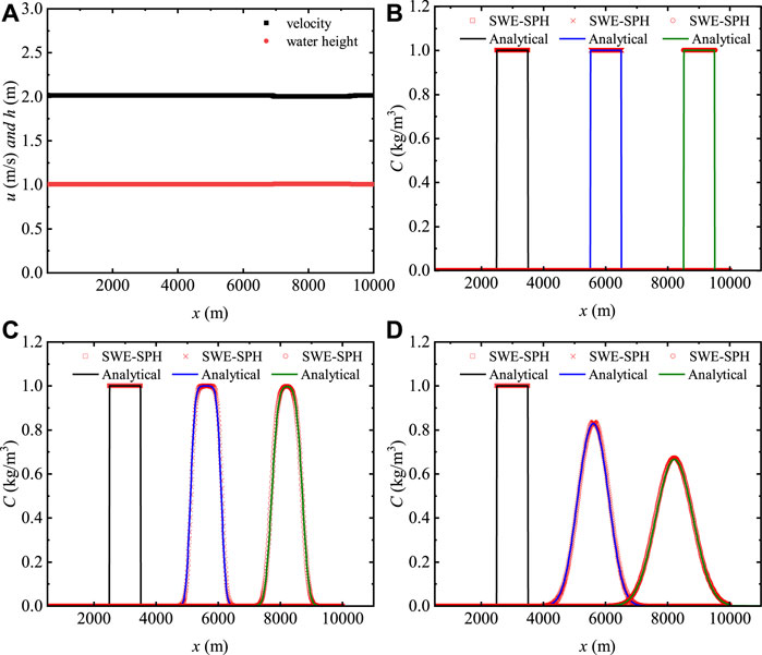
FIGURE 1. Comparison of analytical solutions and SPH-SWE simulation results of 1-D finitely distributed sources (A) Velocity and water height along the x-axis (t = 1,300 s), (B–D) Concentration distribution (t = 0 s, 1,300 s, and 2,600 s respectively).

FIGURE 2

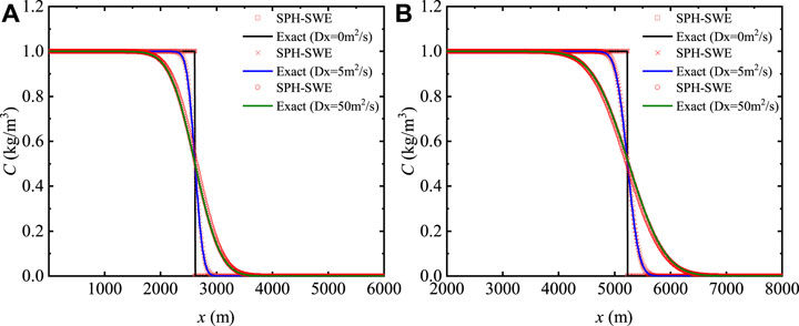
FIGURE 2. Comparison of analytical solutions and SPH-SWE simulation results of a 1-D time-continuum distribution source. (A,B) Concentration distribution (t = 1300 s and 2600 s respectively).

3.2 Dam-Break Flow

The case of pure convective diffusion ignoring gradient diffusion in dry and wet dam-break flows is simulated in this part with the diffusion coefficient of 0 m² s⁻¹. The computational domain is a rectangular flat-bottomed river bed with a length of 2000 m. The particle spacing of the dry river bed is taken as 10 m and that of the upper reaches of the wet river bed is 10 m, and the downstream is 20 m.

The upstream water depth and pollutant concentration of the wet river bed are 10 m and 0.7 Kg m⁻³, and the downstream water depth and pollutant concentration are 5 m and 0.5 Kg m⁻³, respectively. The water depth and pollutant concentration upstream of the dry riverbed are the same as the initial parameters of the wet riverbed, and there is no water downstream. The migration process of the pollutant concentration is simulated for dry and wet river bed dam breaks, and the results of the SPH-SWE formula are compared with the analytical solution (Stoker, 1948) for verification. The SPH-SWE result of the dam break on the dry river bed is shown in Figure 3. It could be seen from Figure 3A that when time t = 50 s, the upstream water depth is 10 m, and near 450 m, the water depth decreases with a small curvature. The result is continuous and smooth. The water depth gradient of the initial conditions at the intermediate position is relatively large, but there is no numerical oscillation, and the result is relatively stable. In Figure 3B, since the gradient diffusion effect is not considered, the pollutant concentration value is always 0.7 Kg m⁻³, and the calculation result is reasonable.

FIGURE 3

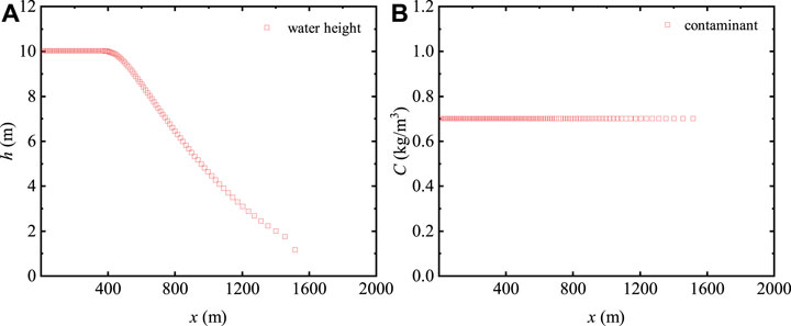
FIGURE 3. Calculation results of a dry bed t = 50 s: water depth (A) and concentration (B).

The simulation results of dam breaks with the wet bed are shown in Figure 4. Figures 4A, B, respectively, present the water depth and concentration distribution of the wet river bed dam break at time t = 50 s. In Figure 4A, it could be seen that the water depth at the upstream and downstream positions is 10 and 5 m, respectively. The result of the water depth is close to the analytical solution, and there is no numerical oscillation at the discontinuity. The simulation result of the SPH-SWE formula is smoother than the analytical solution. In Figure 4B, it could be seen that the concentration drops abruptly when the horizontal displacement is close to 1,200 m, from the upstream concentration value of 0.7 Kg m⁻³ to the downstream value of 0.5 Kg m⁻³. The numerical results are consistent with the analytical ones. It is further verified that the 1-D SPH-SWE diffusion model is reasonable and has good numerical stability.

FIGURE 4

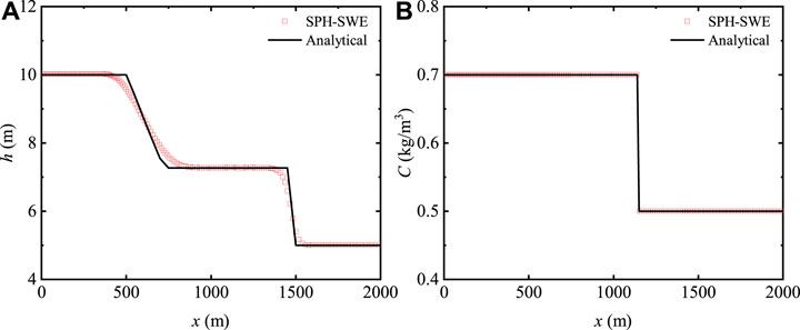
FIGURE 4. Calculation results of a wet bed t = 50 s: water depth (A) and concentration (B).

3.3 Uniform Flow in Two Dimensions

The computational domain of the two-dimensional uniform flow is a rectangular upside-slope channel with a size of 1,200 × 400 m and a slope value of 0.001m discretized by the fluid particle spacing of 1 m. Then, the initial velocity and water depth are set to 2.9 m s⁻¹ and 5 m, respectively. Open boundary and closed boundary conditions are encountered in the simulation, and no-slip boundary conditions are set for the closed boundary on the left and right banks. The fluid movement direction of the two-dimensional uniform flow sets the inflow and outflow boundaries. The particle velocity, water depth, and concentration of the inflow and outflow are 2.9 m s⁻¹, 5 m, and 0 Kg m⁻³ , respectively. The migration and diffusion law distribution of circular instantaneous pollution non-point sources with pollutant diffusion coefficients of 0 and 10,000 m² s⁻¹ are studied. Figure 5 shows the numerical results of the SPH-SWE formula for the circular instantaneous non-point source pollutant concentration at different time instants without considering the diffusion effect. The blue area in Figure 5 represents that the concentration of pollutants in the fluid is 0 Kg m⁻³. It could be seen that the pollutant is red in the movement of the fluid with time, and the concentration value is 1 Kg m⁻³. It shows that the diffusion effect is not involved in the process of pollutant dissemination, and the distance from the instantaneous surface source diffusion to the rightmost edge position (the red dotted line in the figure) is the product of the speed of the 2-D uniform flow and the time t, x = x₀ + ut, corresponding to the different positions. It could explain the rationality of the present numerical results.

FIGURE 5

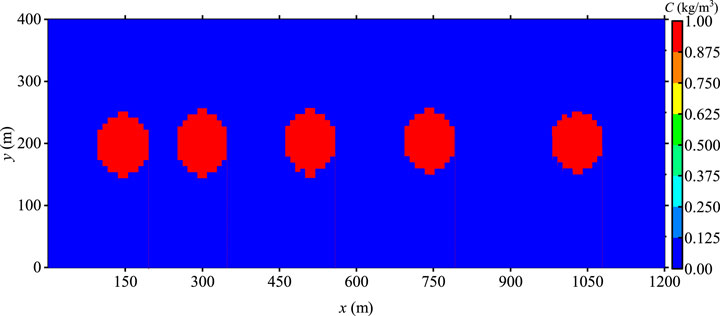
FIGURE 5. Calculation result of the two-dimensional uniform flow condition D = 0 m²s⁻¹.

With the diffusion coefficient D = 10,000 m² s⁻¹, Figure 6 shows the results of the circular instantaneous non-point source pollutant concentration at the different time instants. By comparing the results of Figures 5, 6, it could be seen that the center of the circular instantaneous non-point source pollutant in Figure 6 is at the same position as the center of the circle in Figure 5. Due to the gradient diffusion effect, at time t = 50, 120, 200, and 300 s, the distance from the center of the pollutant circle to the diffusion edge in Figure 6 is farther than that in Figure 5. The concentration value changes with time; the concentration value is less than 1 Kg m⁻³ and the edge positions (the red dotted line in the figure) are, respectively. The concentration value near the center of the pollution source is always at its peak state, and its concentration value decreases from the center of the circle to the edge position, satisfying the law of concentration diffusion. Reasonable results verify that the SPH-SWE diffusion model also has reasonable capturing of pollutants in the two-dimensional fluid movement. It proves that the SPH-SWE formula has advantages in simulating the migration and diffusion processes of conservative pollutants, and there is no need to consider the solution of the migration term in the transport equation. Only using the numerical discretization technique of the SPH method to approximate the diffusion term with the second-order derivative could simulate and predict the diffusion process of pollutants, showing that the SPH-SWE method has good advantages in simulating the diffusion of conservative pollutants.

FIGURE 6

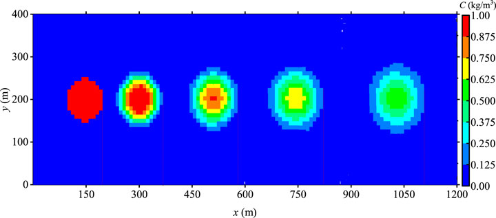
FIGURE 6. Calculation result of the two-dimensional uniform flow condition D = 10,000 m²s⁻¹.

4 Application

This part explains the Nanmenxia Reservoir in Huzhu County, Qinghai Province. The elevation of the reservoir’s total area is above 2, 700 m, and the area is about 218 Km². The maximum dam height is 27.50 m, the crest length is 467 m, and the crest elevation is 2, 772.5 m. The topographic map is shown in Figure 7. Here, X, Y, and Z are the three-dimensional coordinates of the topographic data of the Nanmenxia Reservoir.

FIGURE 7

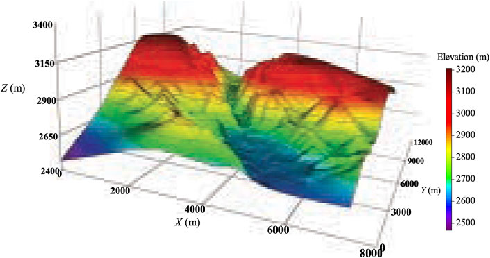
FIGURE 7. Topographic map of the Nanmenxia Reservoir.

Zheng (2017) has carried out a numerical study of the dam-break flow in the Nanmenxia Reservoir area, simulating the full-break (breaking width of 467 m) and partial-break (breaking width of 117 m) conditions. The fluid-particle spacing is 10, 15, and 20 m, respectively. The water levels and velocities at different locations are discussed, and a convergence analysis is conducted. Through the analysis of the numerical data, it is concluded that the SPH-SWE model is convergent and reasonable. The present study mainly conducts an extended study of this case. When the simulated diffusion coefficient is taken as 0 m² s⁻¹, the variable diffusion coefficient and the migration and diffusion process of pollutants in the watershed are calculated after the Nanmenxia Reservoir breaks instantaneously. The rest of the initial conditions of water movement and parameter settings are the aforementioned parameters. The simulation area of the Nanmenxia Reservoir shows that the riverbed gradient is 0.012, and the roughness is 0.024. The initial fluid area is arranged between the x coordinate of 1800 m–2,500 m and the y coordinate of 8,200 m–9,000 m. The fluid-particle spacing is 20 m, with a total of 2,664 fluid particles. The initial water depth and velocity are 0.15 m and 0 m s⁻¹, respectively, and the particle spacing of the river bed is also taken as 30 m, with a total of 89,167 river bed particles. The initial position of the contaminants is a circular area source with x and y coordinates of 2, 450 m and 9, 255 m and a radius of 100 m. The concentration is 1 Kg m⁻³, and the initial concentration in the remaining areas is 0 Kg m⁻³. The total simulation time is taken as 600 s. A detailed discussion on the water flow movement process of the Nanmenxia Reservoir dam break has been made, and it was verified that the particle spacing of 20 m is feasible. This study focuses on the study of the distribution of pollutant concentration fields in the calculation area of the Nanmenxia Reservoir during the instantaneous total collapse. The simulation results of the pollutant concentration of the Nanmenxia Reservoir with D = 0 m² s⁻¹ and variable diffusion coefficients are discussed as follows. The variable diffusion coefficient formula is as follows:

$\left\{\begin{array}{c}{D}_L=6.09\times u^{\ast }\times d\hfill \\ D_T=0.6\times u^{\ast }\times d\hfill \end{array}\right.,(18)$

and the second-order tensors D_xx, D_xy, D_yx, and D_yy corresponding to the diffusion coefficient are

$\left\{\begin{array}{c}{D}_{xx}=D_T+\left(D_L-D_T\right)\frac{{\bar{u}}^2}{V^2}\hfill \\ D_{xy}=D_{yx}=\left(D_L-D_T\right)\frac{\bar{u}\bar{v}}{V^2}\hfill \\ D_{yy}=D_T+\left(D_L-D_T\right)\frac{{\bar{u}}^2}{V^2}\hfill \end{array}\right..(19)$

where D_L and D_T are the lateral and longitudinal diffusion coefficients, respectively, and u* is the frictional velocity of the river bed, which could be calculated according to the river bed gradient and water depth; $V=\sqrt{{\bar{u}}^2+{\bar{v}}^2}$ is the square root of the velocity.

Figure 8 shows the migration and diffusion results of the concentration of pollutants in the dam break of the Nanmenxia Reservoir when the diffusion coefficient is set to 0 m² s⁻¹ at time t = 600 s. It shows that when the simulation time reaches 600 s, the fluid has entered the wide plain area downstream. The pollutants are located in the middle of the river, against the direction of the water flow, such as the red area with the larger velocity. The red area of the concentration distribution already occupies about 1/3 of the fluid area at time t = 600 s, and its shape is roughly the same as the curved shape of the river, indicating that the uneven terrain will also affect the spread of pollutants. It could be found that the pollutants in the research basin are mainly related to the velocity of the water flow. The premise of this case assumes that the diffusion coefficient is 0 m² s⁻¹, implying that the pollutant is only related to the trajectory of the fluid particles in the transportation process, that is to say, only the migration process of the pollutant is considered. As it is assumed that water in the dam of Nanmenxia Reservoir collapses instantly, and with the ups and downs of the topography, the concentration of pollutants will be discontinuous. Because the diffusion coefficient is assumed to be zero, the concentration is not continuous. In actual situations, the spreading and diffusion process of pollutants in water bodies will be related to factors such as the concentration diffusion coefficient and attenuation coefficient of the river and such discontinuities will not occur in the concentration of pollutants.

FIGURE 8

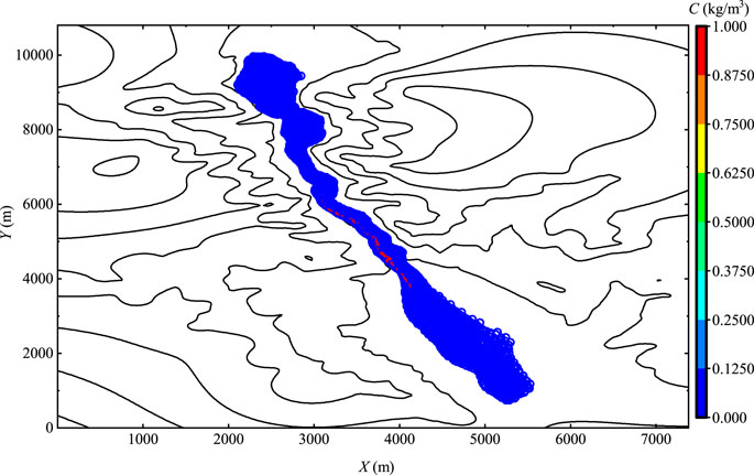
FIGURE 8. Pollutant concentration distribution map after the Nanmenxia dam break (D = 0 m² s⁻¹).

It could be found from Eqs. 18, 19 that the variable diffusion coefficient is calculated based on the river bed gradient, fluid velocity, and water depth. Therefore, each fluid particle in the study area has its own diffusion coefficient. The diffusion process of pollutants is researched and analyzed by solving the variable diffusion coefficient. Figure 9 and Figure 10 show the numerical results of the pollutant concentration with the variable diffusion coefficient at time t = 600 s. It could be noted that there is a large red area in the middle of the river channel with a peak concentration of 0.076 Kg m⁻³, and a small red area in the middle of the downstream river channel with a peak concentration of 0.068 Kg m⁻³. It could be seen that regardless of whether the larger red area or the smaller red area, the concentration value is continuous, the concentration value decreases sequentially from large to small, and there is no jump-type discontinuous distribution of the pollutant concentration. The density values on the left and right sides of the density value of each color gradation are the density values of the adjacent color gradations. Generally divided into four situations, in the downstream plain area, the left is high and the right is low; in the upstream reservoir area, the left is low and the right is high; in the middle area of the river channel, the left and the right are low; and in the yellow area surrounded by two red areas, the left and the right are high and the middle is low. Second, there is no numerical singularity of the pollutant concentration in the whole calculation process, which ensures the non-negativity of the concentration value. The calculation result is stable, and the simulation result conforms to the migration and diffusion laws of pollutants in the actual river.

FIGURE 9

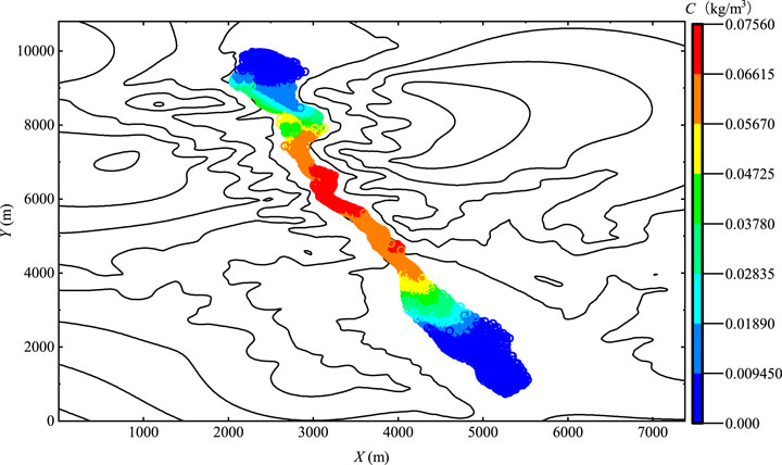
FIGURE 9. Pollutant concentration distribution map after the Nanmenxia dam break under variable diffusion coefficients.

FIGURE 10

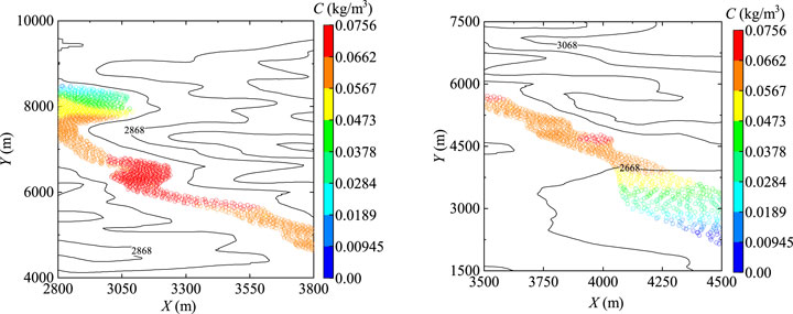
FIGURE 10. Peak contaminant concentration area.

Since the variable diffusion coefficient is related to topography, water flow velocity, and water depth, it more truly describes the migration and diffusion process of soluble conservative pollutants in the actual wide and shallow water flow, verifying that the SPH-SWE diffusion model simulates the pollutants in the actual terrain. Concentration diffusion has good stability, and the SPH-SWE method has a high research value in the prediction of the pollutant transportation process.

5 Conclusion

Cleary and Monaghan (1999) proposed a SPH heat conduction model, which provides a mature numerical format for the discrete solution of the second-order diffusion term in the heat conduction formula. Based on the previous work, this article further expands the application of the SPH-SWE formula. The simulation of the migration and diffusion of pollutants in shallow water is realized, and the diffusion process of soluble inert pollutants in the river is simulated and predicted. The research results of this article are summarized as follows:

• Adding the transport equation for conservative pollutants in the open-source program, uniform flow and classic dam-break flows are simulated in 1 D and 2 D. The numerical results are highly consistent with the analytical solutions, which prove the accuracy of the SPH-SWE model in predicting the propagation process of pollutants in rivers with actual terrain.

• The SPH-SWE formula is used to study the migration laws of soluble and insoluble pollutants in rivers. In the simulation process, negative concentration values could be avoided, which verifies the stability of the model and the rationality of the pollutant numerical results. It proves that the SPH-SWE method has great potential in simulating the spread of pollutants.

The open-source code is used to study the migration and diffusion of soluble conservative pollutants in shallow water, which expands the application fields of the SPH-SWE method. However, the problems of boundary and calculation efficiency are not considered in detail. In the boundary treatment, the concentration diffusion effect near the solid wall boundary is not fully considered. Second, Wu et al. (2020) performed parallel processing on the open-source shallow water code, but we have not added parallel computing. The next step is to add parallel computing to further improve its efficiency. The content of this research has some shortcomings, but we hope to provide some experience for the future related research study. It should be noted that the initial pollutants in the present simulation are simple, and they are much more complex in real life. Complex and realistic pollution sources will be taken into consideration in future research.

Data Availability Statement

The original contributions presented in the study are included in the article/Supplementary Material, further inquiries can be directed to the corresponding authors.

Author Contributions

LT: methodology, visualization, validation, formal analysis, investigation, writing—original draft, and writing—review and editing; SG: supervision, investigation, and writing—review and editing; YW: investigation; HW: investigation; CZ investigation and writing—review and editing.

Funding

This research work was supported by the National Natural Science Foundation of China (No. 51869025) and the Open Research Fund Program of the State Key Laboratory of Hydroscience and Engineering, Tsinghua University (No. SKLHSE-2021-B-04).

Conflict of Interest

The authors declare that the research was conducted in the absence of any commercial or financial relationships that could be construed as a potential conflict of interest.

Publisher’s Note

All claims expressed in this article are solely those of the authors and do not necessarily represent those of their affiliated organizations, or those of the publisher, the editors, and the reviewers. Any product that may be evaluated in this article, or any claim that may be made by its manufacturer, is not guaranteed or endorsed by the publisher.

References

Ata, R., and Soulaïmani, A. (2005). A Stabilized Sph Method for Inviscid Shallow Water Flows. Int. J. Numer. Meth. Fluids 47, 139–159. doi:10.1002/fld.801

CrossRef Full Text | Google Scholar

Bai, B., Rao, D., Xu, T., and Chen, P. (2018). Sph-fdm Boundary for the Analysis of thermal Process in Homogeneous media with a Discontinuous Interface. Int. J. Heat Mass Transfer 117, 517–526. doi:10.1016/j.ijheatmasstransfer.2017.10.004

CrossRef Full Text | Google Scholar

Bonet, J., and Lok, T.-S. L. (1999). Variational and Momentum Preservation Aspects of Smooth Particle Hydrodynamic Formulations. Comp. Methods Appl. Mech. Eng. 180, 97–115. doi:10.1016/s0045-7825(99)00051-1

CrossRef Full Text | Google Scholar

Capecelatro, J. (2018). A Purely Lagrangian Method for Simulating the Shallow Water Equations on a Sphere Using Smooth Particle Hydrodynamics. J. Comput. Phys. 356, 174–191. doi:10.1016/j.jcp.2017.12.002

CrossRef Full Text | Google Scholar

Chang, T.-J., Kao, H.-M., Chang, K.-H., and Hsu, M.-H. (2011). Numerical Simulation of Shallow-Water Dam Break Flows in Open Channels Using Smoothed Particle Hydrodynamics. J. Hydrol. 408, 78–90. doi:10.1016/j.jhydrol.2011.07.023

CrossRef Full Text | Google Scholar

Chang, Y.-S., and Chang, T.-J. (2017). Sph Simulations of Solute Transport in Flows with Steep Velocity and Concentration Gradients. Water 9, 132. doi:10.3390/w9020132

CrossRef Full Text | Google Scholar

Cleary, P. W., and Monaghan, J. J. (1999). Conduction Modelling Using Smoothed Particle Hydrodynamics. J. Comput. Phys. 148, 227–264. doi:10.1006/jcph.1998.6118

CrossRef Full Text | Google Scholar

Colagrossi, A., and Landrini, M. (2003). Numerical Simulation of Interfacial Flows by Smoothed Particle Hydrodynamics. J. Comput. Phys. 191, 448–475. doi:10.1016/s0021-9991(03)00324-3

CrossRef Full Text | Google Scholar

Gingold, R. A., and Monaghan, J. J. (1977). Smoothed Particle Hydrodynamics: Theory and Application to Non-spherical Stars. Monthly notices R. astronomical Soc. 181, 375–389. doi:10.1093/mnras/181.3.375

CrossRef Full Text | Google Scholar

Gu, S., Zheng, X., Ren, L., Xie, H., Huang, Y., Wei, J., et al. (2017). Swe-sphysics Simulation of Dam Break Flows at South-Gate Gorges Reservoir. Water 9, 387. doi:10.3390/w9060387

CrossRef Full Text | Google Scholar

Hernquist, L., and Katz, N. (1989). TREESPH - A Unification of SPH with the Hierarchical Tree Method. ApJS 70, 419–446. doi:10.1086/191344

CrossRef Full Text | Google Scholar

Hirschler, M., Säckel, W., and Nieken, U. (2016). On Maxwell-Stefan Diffusion in Smoothed Particle Hydrodynamics. Int. J. Heat Mass Transfer 103, 548–554. doi:10.1016/j.ijheatmasstransfer.2016.07.061

CrossRef Full Text | Google Scholar

Lastiwka, M., Basa, M., and Quinlan, N. J. (2009). Permeable and Non-reflecting Boundary Conditions in Sph. Int. J. Numer. Meth. Fluids 61, 709–724. doi:10.1002/fld.1971

CrossRef Full Text | Google Scholar

Li, J., Liu, H., Gong, K., Tan, S. K., and Shao, S. (2012). Sph Modeling of Solitary Wave Fissions over Uneven Bottoms. Coastal Eng. 60, 261–275. doi:10.1016/j.coastaleng.2011.10.006

CrossRef Full Text | Google Scholar

Liang, D., Jian, W., Shao, S., Chen, R., and Yang, K. (2017). Incompressible Sph Simulation of Solitary Wave Interaction with Movable Seawalls. J. Fluids Structures 69, 72–88. doi:10.1016/j.jfluidstructs.2016.11.015

CrossRef Full Text | Google Scholar

Liu, G.-R., and Liu, M. B. (2003). Smoothed Particle Hydrodynamics: A Meshfree Particle Method (World Scientific).

Google Scholar

Liu, W., Hou, Q., Lian, J., Zhang, A., and Dang, J. (2020). Coastal Pollutant Transport Modeling Using Smoothed Particle Hydrodynamics with Diffusive Flux. Adv. Water Resour. 146, 103764. doi:10.1016/j.advwatres.2020.103764

CrossRef Full Text | Google Scholar

Long, T., Hu, D., Wan, D., Zhuang, C., and Yang, G. (2017). An Arbitrary Boundary with Ghost Particles Incorporated in Coupled FEM-SPH Model for FSI Problems. J. Comput. Phys. 350, 166–183. doi:10.1016/j.jcp.2017.08.044

CrossRef Full Text | Google Scholar

Lucy, L. B. (1977). A Numerical Approach to the Testing of the Fission Hypothesis. astronomical J. 82, 1013–1024. doi:10.1086/112164

CrossRef Full Text | Google Scholar

Monaghan, J. J. (1994). Simulating Free Surface Flows with Sph. J. Comput. Phys. 110, 399–406. doi:10.1006/jcph.1994.1034

CrossRef Full Text | Google Scholar

Monaghan, J. J. (2005). Smoothed Particle Hydrodynamics. Rep. Prog. Phys. 68, 1703–1759. doi:10.1088/0034-4885/68/8/r01

CrossRef Full Text | Google Scholar

Nguyen, M. T., Aly, A. M., and Lee, S.-W. (2018). Isph Modeling of Natural Convection Heat Transfer with an Analytical Kernel Renormalization Factor. Meccanica 53, 2299–2318. doi:10.1007/s11012-018-0825-3

CrossRef Full Text | Google Scholar

Pu, J. H., Cheng, N.-S., Tan, S. K., and Shao, S. (2012). Source Term Treatment of Swes Using Surface Gradient Upwind Method. J. hydraulic Res. 50, 145–153. doi:10.1080/00221686.2011.649838

CrossRef Full Text | Google Scholar

Ramos-Becerra, G., Moulinec, C., Emerson, D., and Gu, X. (2009). “Inlet-outlet Boundary Conditions and Truly Incompressible Sph,” in Proc 4th ERCOFTAC SPHERIC workshop, Nantes, France, 226–231.

Google Scholar

Randles, P. W., and Libersky, L. D. (1996). Smoothed Particle Hydrodynamics: Some Recent Improvements and Applications. Comp. Methods Appl. Mech. Eng. 139, 375–408. doi:10.1016/s0045-7825(96)01090-0

CrossRef Full Text | Google Scholar

Rao, D., and Bai, B. (2020). Study of the Factors Influencing Diffusive Tortuosity Based on Pore-Scale Sph Simulation of Granular Soil. Transp Porous Med. 132, 333–353. doi:10.1007/s11242-020-01394-0

CrossRef Full Text | Google Scholar

Rezavand, M., Zhang, C., and Hu, X. (2020). A Weakly Compressible Sph Method for Violent Multi-phase Flows with High Density Ratio. J. Comput. Phys. 402, 109092. doi:10.1016/j.jcp.2019.109092

CrossRef Full Text | Google Scholar

Rodriguez-Paz, M., and Bonet, J. (2005). A Corrected Smooth Particle Hydrodynamics Formulation of the Shallow-Water Equations. Comput. Structures 83, 1396–1410. doi:10.1016/j.compstruc.2004.11.025

CrossRef Full Text | Google Scholar

Stoker, J. J. (1948). The Formation of Breakers and Bores the Theory of Nonlinear Wave Propagation in Shallow Water and Open Channels. Comm. Pure Appl. Math. 1, 1–87. doi:10.1002/cpa.3160010101

CrossRef Full Text | Google Scholar

Tartakovsky, A. M., Meakin, P., Scheibe, T. D., and Eichler West, R. M. (2007). Simulations of Reactive Transport and Precipitation with Smoothed Particle Hydrodynamics. J. Comput. Phys. 222, 654–672. doi:10.1016/j.jcp.2006.08.013

CrossRef Full Text | Google Scholar

Vacondio, R., Rogers, B. D., Stansby, P. K., and Mignosa, P. (2012). Sph Modeling of Shallow Flow with Open Boundaries for Practical Flood Simulation. J. Hydraul. Eng. 138, 530–541. doi:10.1061/(asce)hy.1943-7900.0000543

CrossRef Full Text | Google Scholar

Vacondio, R. (2010). Shallow Water and Navier-Stokes Sph-like Numerical Modelling of Rapidly Varying Free-Surface Flows.

Google Scholar

Wu, Y., Tian, L., Rubinato, M., Gu, S., Yu, T., Xu, Z., et al. (2020). A New Parallel Framework of Sph-Swe for Dam Break Simulation Based on Openmp. Water 12, 1395. doi:10.3390/w12051395

CrossRef Full Text | Google Scholar

Xia, X., Liang, Q., Pastor, M., Zou, W., and Zhuang, Y.-F. (2013). Balancing the Source Terms in a Sph Model for Solving the Shallow Water Equations. Adv. Water Resour. 59, 25–38. doi:10.1016/j.advwatres.2013.05.004

CrossRef Full Text | Google Scholar

Zhang, A.-m., Sun, P.-n., Ming, F.-r., and Colagrossi, A. (2017a). Smoothed Particle Hydrodynamics and its Applications in Fluid-Structure Interactions. J. Hydrodyn 29, 187–216. doi:10.1016/s1001-6058(16)60730-8

CrossRef Full Text | Google Scholar

Zhang, C., Hu, X. Y., and Adams, N. A. (2017b). A Weakly Compressible Sph Method Based on a Low-Dissipation Riemann Solver. J. Comput. Phys. 335, 605–620. doi:10.1016/j.jcp.2017.01.027

CrossRef Full Text | Google Scholar

Zhang, C., Rezavand, M., and Hu, X. (2021a). A Multi-Resolution Sph Method for Fluid-Structure Interactions. J. Comput. Phys. 429, 110028. doi:10.1016/j.jcp.2020.110028

CrossRef Full Text | Google Scholar

Zhang, C., Rezavand, M., Zhu, Y., Yu, Y., Wu, D., Zhang, W., et al. (2021b). Sphinxsys: An Open-Source Multi-Physics and Multi-Resolution Library Based on Smoothed Particle Hydrodynamics. Comp. Phys. Commun. 267, 108066. doi:10.1016/j.cpc.2021.108066

CrossRef Full Text | Google Scholar

Zhang, C., Wang, J., Rezavand, M., Wu, D., and Hu, X. (2021c). An Integrative Smoothed Particle Hydrodynamics Method for Modeling Cardiac Function. Comp. Methods Appl. Mech. Eng. 381, 113847. doi:10.1016/j.cma.2021.113847

CrossRef Full Text | Google Scholar

Zheng, X. P. (2017). The application of the sph method in dam-break water flow simulation. Qinghai Provence, China: Qinghai University.

Google Scholar

Zhu, Y., and Fox, P. J. (2001). Smoothed particle hydrodynamics model for diffusion through porous media. Transport in Porous Media 43, 441–471. doi:10.1023/a:1010769915901

CrossRef Full Text | Google Scholar