 Hira Shaukat
 Ken C. Flower
 Matthias Leopold
94% of researchers rate our articles as excellent or good
Learn more about the work of our research integrity team to safeguard the quality of each article we publish.
Find out more
ORIGINAL RESEARCH article
Front. Environ. Sci., 19 July 2022
Sec. Drylands
Volume 10 - 2022 | https://doi.org/10.3389/fenvs.2022.883533
This article is part of the Research TopicCurrent Insights in DrylandsView all 13 articles
Leptospermum sp. with dihydroxyacetone in their nectar are a source of high-value medicinal honey production and can provide income from agriculturally marginal lands. The current study was from two newly planted Leptospermum nitens sites, one with duplex soil and the other in deep sandy soil, in the low rainfall areas of the south-west of Western Australia, with the aim of identifying key soil parameters influencing the plantation’s survival and growth. Electromagnetic induction (EMI) at different depths was used to investigate the possible impact of soil variability on the Leptospermum nitens plantations. Two EMI surveys were conducted at each site, at different times of the year, to account for soil moisture variability (relatively dry and wet conditions). A least-square inversion algorithm was used to determine true electrical conductivities at three different soil depths (0–0.5, 0.5–0.8, and 0.8–1.6 m) to produce quasi-3D maps of soil inverted electrical conductivity. Corresponding soil samples from each depth were used for the physico-chemical analysis of soil parameters and to develop laboratory-based electrical resistivity to soil volumetric moisture calibrations with R2 values between 0.95 and 0.99. Shrub survival and growth (canopy diameter) were estimated using unmanned aerial vehicle (UAV) images and machine learning. Comparing EMI soil mapping with UAV imagery results showed significantly greater shrub survival and growth (p < 0.001) in areas with higher ECa ranges of 12–24 mS m−1 at the variable textured site and 6–9 mS m−1 at the uniformly sandy site. Overall, the variable textured site, with an 82% survival rate, had a significantly higher shrub count and larger plants than the uniformly sandy site, with a 75% survival rate. A principal component analysis (PCA) identified inverted EC to be strongly correlated with soil moisture > pH > soil texture. Such soil mapping may be a robust and effective method for risk assessment of new shrub plantations.
Land degradation and associated dry land salinity is a major challenge in Australia caused by the removal of native vegetation (Stirzaker et al., 2002). Land clearing and intensive cereal/annual pasture rotations have exposed surface soils to excessive wind and water erosion, often in combination with dryland salinity issues, under semi-arid rain-fed conditions (Lamb, 2014). In response, most farmers have adopted no-tillage cropping practices with crop residue retention (D’Emden et al., 2008). According to the latest estimate, more than 1 million ha of south-west Western Australia (WA) is affected by salinity resulting in the loss of at least $519 million per year (Australian Bureau of Statistics, 2002; Furby et al., 2010). Indeed, the current scale of this degradation problem now requires landscape level mitigation responses such as reforestation (George et al., 2012). Species identified for mitigation are mainly selected based on their ecological role; however, estimated costs of such reforestation plans often exceed the value of the land (Lamb, 2014; Harper et al., 2017). A major factor affecting large-scale reforestation is to obtain an impactful hydrological response without displacing farm production (Harper et al., 2014). Therefore, market-driven reforestation has the potential to encourage the integration of perennial plants into existing farming systems (Mendham et al., 2011). A recent report on high-value honey derived from Leptospermum species in Australia has identified the opportunity for bioactive honey production at a commercial scale, either by diversifying traditional agricultural regions such as the WA wheatbelt region or by using unproductive lands through revegetation-focused projects (Cokcetin et al., 2019).
Leptospermum is a member of the Myrtaceae family, with 300 genera and more than 3,800 species, with 85 out of 88 identified Leptospermum species in this region being native to Australia (Bean, 1992, 2004), and 15 of which are native to WA. Leptospermum is endemic Australian species (Thompson, 1989), closely related to the widely studied and commercially successful L. scoparium, found in Tasmania, the north-west mainland of Australia, and in New Zealand (Porter and Wilkins, 1999; Stephens et al., 2005; Adams et al., 2009; Wicaksono et al., 2016; Thrimawithana et al., 2019). These species are renowned for their essential oils and nectar production for honey and are also used as ornamental shrubs. Leptospermum honey is popular for its synergistic impact with common antifungal and antibacterial agents (Lu et al., 2013; Cokcetin et al., 2016). The high/medicinal value of Leptospermum honey is due to the presence of the chemical component methyl glyoxal (MGO), which is formed from its precursor dihydroxyacetone (DHA) (Adams et al., 2008; Mavric et al., 2008). Not all Leptospermum species produce DHA in their nectar. The WA’s species, Leptospermum Nitens (Turcz), has been shown to produce higher DHA and MGO levels than L. scoparium (Williams et al., 2018).
Leptospermum is a common seral shrub in succession to forest. They are usually known as a woody weed of pastures (Burrell, 1965) and are useful for erosion control (Marden and Phillips, 2015), carbon sequestration (Scott et al., 2000; Beets et al., 2014), and vegetation restoration (Marden and Phillips, 2015). Mostly, they are dominant in low fertility, poorly drained environments (Thompson, 1989), grasslands, woodlands, and heathlands (Burrell, 1981; Bennett, 1994). Since these plants can adapt to various soil and climatic conditions (Dodson et al., 1995; Hageer et al., 2017), it is expected that they will be responsive to managed cultivations (Cokcetin et al., 2019). Developing the commercial aspects of this species from an ornamental plant to a pharmacologically active plant can make it a potential priority candidate for agroforestry (Cokcetin et al., 2019).
Site assessments are useful practical tools for planning agricultural land management, but limited information is available regarding the impact of soil variations on the establishment of new native shrub plantations. Electromagnetic induction (EMI) may be a promising tool for soil surveying when establishing new native plantations. EMI sensors, which can take readings at different depths simultaneously, provide the simplest and least expensive method to assess soil variations on a broad scale. These non-invasive sensors measure the contactless bulk soil electrical properties that contribute to the apparent electrical conductivity (ECa). The measured soil Eca is a response to conductive soil parameters such as salt content, soil moisture, organic matter, soil texture, bulk density, stratigraphic layers, or bedrock (van Wesenbeeck and Kachanoski, 1988; Triantafilis et al., 2000; James et al., 2003; Corwin and Lesch, 2013; Doolittle and Brevik, 2014; Dakak et al., 2017). Generally, EMI assessments are used in agriculture (Hedley and Yule, 2009; Hanssens et al., 2019; Arshad et al., 2020; Shaukat et al., 2022) and especially for quantifying the risks related to salinity (Scudiero et al., 2017; Paz et al., 2020; Farzamian et al., 2021). However, Bennett and George (1995) conducted an EMI survey to quantify salinity for the new plantations of Eucalyptus globulus and suggested that this method could be used for assessing soil variations for risk assessments before establishing new plantations.
Moreover, remote sensing methods are becoming mainstream in planning for tree plantations and their management (Charron et al., 2020; Dainelli et al., 2021; Dixon et al., 2021). In particular, drones/unmanned aerial vehicles (UAVs) provide efficient aerial mapping and estimation of deforestation rates, quantifying above ground biomass, monitoring climatic impacts on land use, woodlands, and forest ecosystems, and getting information from the sites that are difficult to reach (Pádua et al., 2017; Raparelli and Bajocco, 2019). A combination of new technologies for both soil and aerial surveys with quick turn-around times can provide data-driven decisions for agroforestry (Pádua et al., 2017).
L. nitens is one of the species identified with the potential of making the unproductive low fertility areas in the “wheatbelt” region of WA a “hot spot” for generating bioactive honey (Cokcetin et al., 2019). Limited information is available on a field scale to understand the impact of soil limitations, such as shallow, saline- or nutrient-deficient soils, on the survival and growth rate of L. nitens. Such information could possibly identify factors correlated to the yield and quality of nectar production for medicinal honey. The hypothesis of the current study was that EMI could be used to identify soil parameters related to L. nitens survival and growth across the two soil types. The overall aim was to develop a robust, rapid, and non-invasive soil mapping system to identify soil parameters influencing the performance of L. nitens for potential commercial cultivation across different soil types. A prognosis for the most suitable soil conditions for commercialization of L. nitens in WA is presented.
Two sites with contrasting soils and newly planted L. nitens shrubs were selected for this study to understand the survival and growth of this species with respect to soil characteristics. The area has a Mediterranean–type climate with mild, wet winters and hot, dry summers. A Dualem-1HS EMI sensor was used for two soil surveys at each site, at two different times of the year, to include variable (relatively dry and wet) soil moisture conditions. Soil samples were also collected from the study sites to measure soil physical and chemical properties and to develop soil moisture vs. resistivity calibration curves for the different soil depths under laboratory conditions. In addition, shrub count (survival) and shrub canopy diameter (growth) estimation were done using unmanned aerial vehicle–UAV images and machine learning. EMI soil mapping was related to drone imagery results to understand the influence of soil variability on newly planted shrub survival (count) and growth.
This study site is 16 ha located in Mooribin Badgingarra in the Shire of Dandaragan, about 200 km north of Perth (115° 42′ 04.9″ E, 30° 16′ 27.3″ S; Figure 1A). From 1965 to 2021, the recorded mean daily temperature was 7.6°C in July and 34.6°C in January. The average annual rainfall was 530 mm, with 430 mm falling between May and October during the growing season and 100 mm between November and April during summer and autumn, with a mean annual cumulative evapotranspiration rate of 2,376 mm [Badgingarra research station, BADG 009037 (BOM, 2021)]. The soil is classified as an Arenosol by both the Australian classification system (ACS) (Isbell and National Committee on Soil and Terrain, 2021) and the international WRB system (IUSS, 2014). This area is classified under the Northern Kwongan or Sandplains and is recorded as a botanically important area (Griffin, 1994). General soil properties are brown to red-brown sands, which are non-wetting with subsurface acidity. The pH (CaCl2) range is 4.2 in the top 30 cm to 4.9 at 90 cm depth. Mixed farming operations are practiced in this area mostly focused on sheep and beef cattle production along with lupins and wheat crop rotations.

FIGURE 1. Top, location of the study area in Western Australia. Bottom, (A) Site 1–Mooribin and (B) site 2–Kukerin. ECa transects with EMI reading points (red dots) and soil sample locations (gray dots) (C) Leptospermum nitens plant.
This site is 20 ha, located near South Kukerin in the Shire of Dumbleyung, about 320 km south-east of Perth (33° 16′ 6.528″ S 118° 15′ 9.2376″ E; Figure 1B). From 1965 to 2021, mean daily minimum temperatures were 15.4°C in July and 31.2°C in January. Average annual rainfall is around 400 mm, with 300 mm falling from May to October and 100 mm from November to April, with a mean annual cumulative evapotranspiration rate of 1873 mm [Wagin weather station no. 010647 (BOM, 2021)]. The soil is classified as Brown Chromosol based on the Australian classification system (ACS) (Isbell, 2016) or Luvisols based on the international WRB system (IUSS, 2014). General soil features are a combination of sandy topsoils and red-brown sandy loams or sandy clay loams as the subsoil, typical of duplex soils (McKenzie et al., 2004). The pH (CaCl2) range is 4.7 in the top 30 cm to 5.6 at 90 cm depth. The land is mostly used for growing wheat and sheep farming.
L. nitens (Figure 1C) seedlings of 250 mm height and 2 mm stem diameter were planted with a row spacing of 6 and 2 m between plants with an average of ∼830 stems ha−1.
An electromagnetic induction (EMI) sensor (Dualem-1HS) was used for soil surveys at both sites. This is a non-intrusive sensor with a fixed frequency, and it measures the apparent soil electrical conductivity (ECa). This sensor was portable and contained a transmitter coil (Tx) and two pairs of receiver coils (Rx) with depths of exploration (DOE) of 0.3, 0.5, 0.8, and 1.6 m from the surface. The DOE accounts for 70% of the array’s sensitivity (McNeill, 1980) and is determined by orientation and distance between Tx and Rx coils.
Two EMI surveys were conducted at both study sites in June (dry season) and August (after rains) 2019 (Table 1). To conduct the survey, the Dualem-1Hs was placed on a non-conductive polyethylene sled containing a GPS antenna. A light vehicle towed this sled across the fields at a speed of ∼5.5 ms−1. A recording was taken every two seconds, and each point was georeferenced with a horizontal accuracy of less than 0.5 m using the Beacon DGPS function of the Hemisphere GPS R130 unit.

TABLE 1. Summary of EMI field surveys.
Soil samples for laboratory analysis were taken up to a depth of 1 m. The sample locations were chosen using the initial EMI survey, where uniform ECa areas were identified using natural breaks classification in QGIS software (QGIS.org, 2022). There were twelve soil sample locations at Mooribin and nine soil samples at Kukerin (Figure 1). The soil samples were collected using a percussion drill rig with an 8 cm diameter and 1 m long thick steel probe immediately after the surveys in August 2019. The soil samples were bulked by depth into 0–0.5, 0.5–0.8, and 0.8–1 m depths, which broadly corresponded to the main soil horizon boundary of the duplex soils at Kukerin.
Laboratory analysis included: gravimetric moisture content, particle size analysis (PSA) using laser diffraction, pH (CaCl2), electrical conductivity of soil saturated paste (ECe), cation exchange capacity (CEC), exchangeable aluminum (Al), potassium (K), calcium (Ca), magnesium (Mg), and sodium (Na) by atomic emission spectrometry with inductively coupled plasma (ICP–OES) using Perkin Elmer Optima 7300DV optical emission spectrometer (Nicia et al., 2018), extractable phosphorus (P) using colorimetric analysis–0.5 M NaHCO3 and UV-VIS spectrophotometer, and total carbon and nitrogen using CN elemental analyzer. All measurement techniques followed protocols used by Rayment and Lyons (2011) and McKenzie et al. (2002).
To correlate ECa with soil moisture, laboratory-based calibration curves between volumetric moisture content (θ) and soil bulk electrical resistivity ρr were developed. Since resistivity (R) is inversely related to conductivity(C) (R = 1/C), this simple calibration relation provides reliable estimates of soil moisture status from an ECa map (Leopold et al., 2021). Soil sub samples with similar laboratory ECe (<10 μS m−1 difference) and texture were bulked together to reduce the number of samples for developing volumetric moisture (%) calibration equations. Furthermore, for the Mooribin site, which is uniformly sandy throughout, soil moisture calibrations for all the inverted soil depth slices (0–0.5, 0.5–0.8, and 0.8–1.6 m) were done using the single calibration equation. For the Kukerin site, soil moisture calibration for 0.8–1.6 m depth slice was done using the calibration curve developed from 0.5–0.8 m depth slice soil because this is a duplex soil with similar textural characteristics at these depths (Table 2).

TABLE 2. Summary results of soil analysis for the two study sites.
The resistivity to soil water calibration curves was developed using the same method as described by Shaukat et al. (2022); in brief, a sub-sample of each soil depth was placed in a 10 cm × 6.25 cm × 4 cm plastic container and saturated with deionized water. A bulk density of 1.6 g cm−3 was used for Mooribin and 1.5 g cm−3 for Kukerin. Four electrodes at 1 cm spacing were inserted in the saturated soil sample, with the resistivity measured hourly. The whole setup was placed on an automatic scale (0.00 g) to track the weight difference over time of sample drying in a temperature control room at 25°C.
To validate the accuracy of prediction, this predicted soil moisture content was compared with the moisture content derived from the soil samples, which was converted from gravimetric to volumetric moisture units.
UAV imaging surveys were done at Mooribin on 11 December 2020 and at Kukerin on 12 December 2020 to map the survival (tree counting) and growth (shrub canopy diameter) of planted L. nitens. A DJI M600 6 Rotor drone provided with red, green, and blue (RGB) FC550 (15 mm focal length) camera to capture the images (Supplementary Appendices 1 and 2). UAV imaging was carried out around mid-day under a clear sky at the height of 106 m for Mooribin and 100 m for Kukerin. To improve the positional accuracy of the images, four ground control points (GCPs) were identified using a handheld RTK system and used for dereferencing the photogrammetry processing workflow. Imaging metadata is provided in Supplementary Appendices 1 and 2.
In brief, the EMI data was cleaned, and outliers were removed and then inverted to the depths of 0–0.5, 0.5–0.8, and 0.8–1.6 m. The inverted ECa was used to predict field-scale soil moisture using ERT–EMI power-law calibration equations, as previously described. Then, a deep-learning framework for automatically counting the shrubs in the UAV (drone) images was developed. Statistical analysis was performed to determine the main soil parameters at each site that may influence L. nitens survival and growth. The newly planted L. nitens survival and growth data were then compared across the different soil (ECa) zones/areas within each site to relate shrub performance to soil characteristics/map.
A python-based outlier detection algorithm, “hampel filter”, was used for the EMI field data attributed to any surface metallic objects. The filter works with the configurable moving median window and defined number of standard deviations (Delefortrie et al., 2014; Pearson et al., 2016). Here, we used the size of ten data points with three standard deviations to detect the outlier and replace it with the representative median value. Based on the set threshold, the detected outliers were less than 1% of the data in all the arrays. The code for this filter is available in the GitHub repository (Lewinson, 2019).
ECa obtained from the EMI surveys was a weighted average of conductivity over a full depth of exploration. EM4Soil software (EMTOMO, 2018) package was used to invert these weighted averages to depth-specific conductivities or true conductivities (σ, mS m−1) (Monteiro Santos et al., 2010, 2011), which are further mentioned as inverted EC. The quasi-3D inversion algorithm used was based on the assumption that 1-dimensional variation of true electrical conductivity is constrained by neighboring variations for each measured ECa location (Monteiro Santos, 2004; Monteiro Santos et al., 2011). EM4Soil requires a forward model based on linear cumulative function (CF) (McNeill, 1980) or non-linear full solution (FS) (Frischknecht, 1988). The inversion algorithm uses Occam regularization (Sasaki, 1989, 2001) and a damping factor (λ) to balance between data misfit and smoothness of Electromagnetic conductivity imaging (EMCI). Based on the lowest misfit, RMSE, and highest coefficient of determination between modeled and observed data, best inversion results were obtained using the cumulative function model, S2 algorithm with 0.07 λ for 10 iterations.
For quantitative comparison of field ECa, temperature correction for 25°C was performed using correction factors by Ma et al. (2011). Out of our four Dualem-1Hs arrays, we excluded the top 0.5 PRP (DOE 0.3 m) for not being the true representative of 70% of the EMI signal at the top 0.3 m due to the sensor height (10 cm) above the ground resulting in very low to zero conductivity values. A three-layered inversion model was selected based on the used geophysical arrays (Triantafilis et al., 2013), resulting in depth slices of 00.5, 0.5–0.8, and 0.8–1.6 m. The inverted EC was kriged using a 5 m grid in VESPER (Variogram Estimation and Spatial Prediction plus Error) software (Minasny et al., 2005).
Results of measuring electrical resistivity and conductivity are frequency-dependent. For estimating volumetric soil moisture from inverted EC, the differences in frequency of Dualem-1HS (9 kHz) and laboratory-based electrical resistivity tomography (ERT) measurement (4.16 Hz) were accounted for using the “Modified Portela Model” described by Moura et al. (2018).
Raw UAV images at 1.8 cm ground resolution were stitched together to develop an Orthophoto and a 3D point cloud, followed by 3D data classification to produce a canopy height model (CHM). A machine-learning algorithm called “YOLOv5” was used for the L. nitens plant detection for surviving shrubs count. YOLO refers to “You Only Look Once”, a family of algorithms introduced by Redmon et al. (2016). This algorithm is designed to detect individual objects by drawing bounding boxes and identifying classes of objects such as cars, humans, and signs. Unlike segmentation models such as Unet (Ronneberger et al., 2015), where accurate delineation of objects is an important quality indicator, YOLO deals with classification (identifying if the object is present in the image) and accurate localization of objects (prediction of the bounding box around the required object in the image).
For our deep learning training, bounding box samples were collected in 250 images covering shrubs of various sizes and shapes. The actual training was conducted on 80% of the dataset (200 images, including 1,500 shrubs), and the remainder was used for validation. The trained model was tested in two test areas, with 90 and 5,600 m2, to assess the model performance.
Four quality metrics were used to evaluate the object detection model performance: 1) Precision–the percentage of our correct predictions. 2) Recall–the percentage of all the positive predictions. 3) Intersection of union (IoU)–a value used in object detection to measure the overlap of a predicted vs. actual bounding box for an object, and 4) Mean average precision (mAP)–the average of average precision (AP). AP is calculated for each class and averaged to get the mAP.
For modeling of shrub canopy diameter, shrubs were segmented into pixels using circles and estimating the average intensity of pixels within these circles. Given that the intensity values of the shrub and the bare ground were known, the diameter of the shrub (circle around the plant) was set when the average intensity values within the circles were closer to the bare ground than the shrub. For shrub diameter growth, ground-truthing was done by manually taking the diameter of randomly selected 530 shrubs at the Mooribin site. Diameter from each shrub was measured at three heights; top (1/3 plant), middle (widest part), and bottom (1/3 plant) part of the shrub and locations of the shrubs were noted for comparison.
Principal component analysis (PCA) was used to identify the main soil variables that may influence the L. nitens survival and growth (R Core Team, 2020). The input matrix comprised soil physico-chemical analysis data and related inverted EC from 10 m around the soil sampling points at both sites.
The non-parametric Wilcoxon test was used to test the difference between measured volumetric water content from the soil samples and EMI predicted volumetric water content for each depth slice. The Kruskal–Wallis test was used to compare the modeled (UAV-derived) and manual shrub diameter measurements taken from three parts (top, middle, and bottom) of a plant. This test was also used to compare shrub diameters within the different EMI mapped (inverted EC) soil zones/areas for each site. This test was performed using the R software package (R Core Team, 2020).
ECe values for all the soil samples were less than 200 mS m−1 (Table 2), which indicates that both study sites were non-saline (Simons and Bennett, 2021). In addition, average pH values of Mooribin for all three depth slices ranged from 4.5 to 4.9 (SD 0.1) and in Kukerin from 4.7 to 5.6 (SD 0.4). PSA of all the three depth slices of Mooribin showed it to be a relatively uniform sandy site with a mean of 99% sand (SD 3.6). Kukerin soils showed variable textures both vertically and horizontally, with the topsoil being more sandy to loamy and the subsoils being more loamy (Table 2).
Average CEC (mEq 100 g−1) for all the soil depth slices of Mooribin and Kukerin ranged from 0 to 1.6 (SD 0.5) and 0 to 5 (SD 1), respectively. Similarly, exchangeable Al, Ca, K, Mg, and Na were <1 mEq 100 g−1, and total C and N were <1% in all the depth slices of both sites. BicP (mg kg−1) concentration at Mooribin ranged from 0 to 8 (SD 2.0), 0 to 7 (2.8), and 0 to 10 (SD 4.1) mg kg−1 for depth slices of 0–0.3, 0.3–0.5, and 0.5–1.0 m, respectively, while for Kukerin Bic P ranged from 0 to 4 mg kg−1 throughout all the measured depth slices.
Figure 2 shows the spatial distribution of inverted EC at three depth slices of 0–0.5, 0.5–0.8, and 0.8–1.6 m. For Mooribin, the inversion model misfit was 0.2% with RMSE of 0.2 mS m−1 for the dry season survey and model misfit of 0.6% with RMSE of 0.3 mS m−1 for the wet season survey. For Kukerin, the model misfit was 5.4 with RMSE of 6 mS m−1 for the dry season survey and model misfit of 6% with RMSE of 7 mS m−1 for the wet season survey. Inverted EC in the wet season survey was higher than during the dry season and was lower at Mooribin across the site and along the measured depths (0–9 mS m−1) than at the Kukerin site (0–36 mS m−1). The inverted EC was grouped into three ranges according to the measured values at both sites.
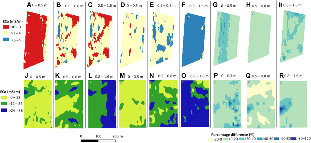
FIGURE 2. Inverted electrical conductivity (EC) at three depths of 0–0.5, 0.5–0.8, and 0.8–1.6 m at the Mooribin site taken on 7 June 2019 [(dry season—A–C)], on 19 August 2019 [(wet season—D–F)]. Percentage difference between the inverted EC of two surveys at three depths (G–I). Similarly, at the Kukerin site on 4 June 2019 [(dry season—J–L) and on 22 August 2019 (wet season—M–O)], and percentage difference maps of two surveys relative to the dry season at three depths (P–R).
At Mooribin, the dry season had the lowest inverted EC range of 0–3 mS m−1 in the top measured depth slice of 0–0.5 m (Figure 2A). The rest of the two depth slices (Figures 2B and C) showed the inverted EC range of 3–6 mS m−1 in most of the area, with patches of 0–3 and 6–9 mS m−1. For the wet season, the top two depth slices, 0–0.5 m (Figure 2B) and 0.5–0.8 m (Figure 2E), mostly had an inverted EC range of 3–6 mS m−1, with some patches of 6–9 mS m−1, especially in the second depth slice. The deepest measured depth slice of 0.8–1.6 m (Figure 2F) had the highest inverted EC range of 6–9 mS m−1. The percentage difference maps (Figures 2G–I) show the change in spatial inverted EC distribution from the dry to wet season, which was most prominent in the top (0–0.5 m, Figure 2F) and the deepest depth slice (0.8–1.6 m, Figure 2H) toward the higher values. Overall, this site showed relatively homogenous inverted EC for the dry and wet season measurements, as expected for uniformly sandy soil.
For Kukerin, the site had a variable spatial distribution of inverted EC, which changed with the season and increased with soil depth. For both seasons, the top depth slice of 0–0.5 m (Figures 2J and M) had the lowest measured inverted EC range of 0–12 mS m−1. However, for the dry season (Figure 2J), the top western part of the field showed an area with mid-range inverted EC of 12–24 mS m−1. The inverted EC appeared to decrease in this top western part of the field in the wet season, compared to the dry season, except for a small area of 12–24 mS m−1 in the bottom east corner (Figure 2M). The highest spatial inverted ECa distribution variability was in the second depth slice for both dry and wet seasons, where most of the area showed the mid-range inverted EC of 12–24 mS m−1. The lower-range inverted EC of 0–12 mS m−1 in the middle of the field in the dry season (Figure 2K) and in the top east corner in the wet season (Figure 2N). During the dry season (Figure 2L), the last depth slice of 0.8–1.6 m showed the west half of the field with mid-range inverted EC (12–24 mS m−1) and the east half with high-range inverted EC (24–36 mS m−1). The last depth slice for the wet season survey (Figure 2O) showed high-range (24–36 mS m−1) inverted EC except for the top east corner.
The percentage difference maps from the dry to wet season survey show a relatively large change in the south-east part of the top depth slice (0–0.5 m; Figure 2P). For the second depth slice (0.5–0.8 m; Figure 2Q), inverted EC increased in the mid-west and decreased in the north part of the site, while in the last depth slice of 0.8–1.6 m (Figure 2R), the maximum increase in inverted EC was in the mid-west part of the field.
Figure 3 shows the resistivity to volumetric moisture power-law curves used for calculating the spatial distribution of volumetric moisture content % (Figure 4) for both sites using the inverted ECa (Figure 2). In the case of Mooribin, the overall volumetric moisture content in the wet season was slightly higher than in the dry season, as expected. The top depth slice of 0–0.5 m (Figures 4A and D) showed the lowest predicted volumetric moisture of 0–6% in the dry season and >3–6% in the wet season in most of the area with the patches of 6–9%. The other two depth slices showed similar moisture distribution patterns, with >3–6% moisture prediction in most of the areas with patches of 6–9% in the dry season (Figures 4B,C) and mostly >6–9% moisture prediction with patches of 9–12% moisture in the wet season (Figures 4E,F). The percentage difference maps showed the maximum soil moisture change in the top depth slice (0–0.5 m; Figure 4G), with <20% change in deeper depths (Figures 4H,I).
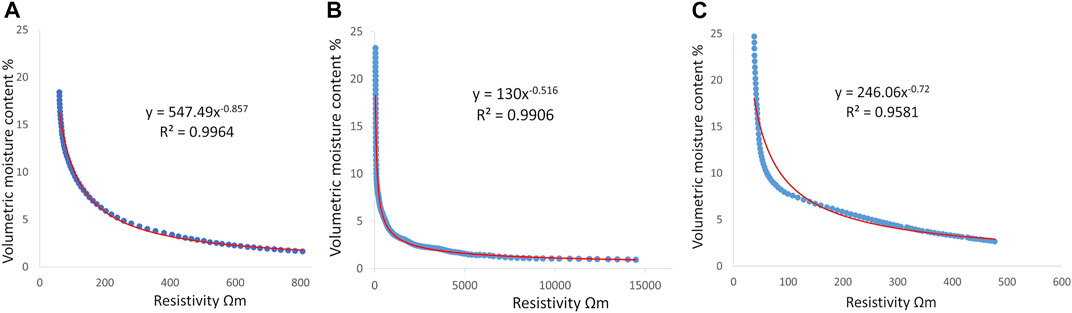
FIGURE 3. Power-law relationships between volumetric moisture content (%) and electrical resistivity (Ωm) for all the depths of Mooribin site (A) and Kukerin site for lower inverted EC range of 0–12 mS m−1 (B) and higher inverted EC range of 12–36 mS m−1 (C). The red line is the fitted power-law.
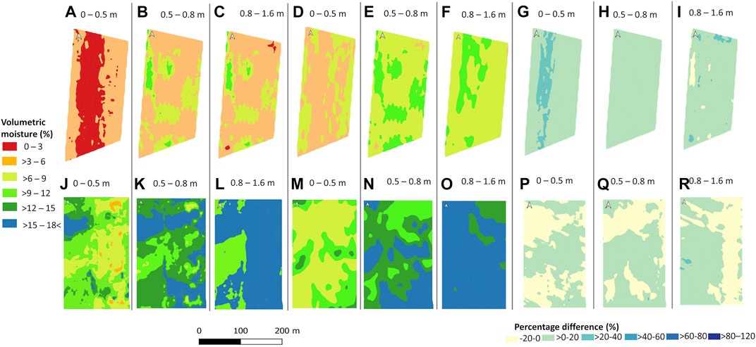
FIGURE 4. Predicted volumetric moisture content based on inverted EC of three depths (0–0.5, 0.5–0.8, and 0.8–1.6 m) at the Mooribin site [(dry season—A–C and wet season—D–F)] and percentage difference between the volumetric moisture content of both seasons (G–I). Similarly, predicted volumetric moisture content at the Kukerin site (dry season—J–L and wet season—M–O) and percentage difference relative to dry season between the volumetric moisture content of both seasons (P–R).
In the case of Kukerin, spatial moisture distribution prediction showed high variability in the top two depth slices of both seasons (Figures 4J, K, M, and N). Broadly, for the dry season, the top depth slice of 0–0.5 m (Figure 4J) had >6–9% moisture in the east half and >9–12% moisture in the west half of the field, except for the top west part with higher moisture prediction of >12–15%. In the wet season, the top depth slice of 0–0.5 m (Figure 4M) had the low-range (>6–9%) moisture in most of the area except for the middle and bottom east corner with mid-range (>9–12%) moisture. For the second depth slice of 0.5–0.8 m, in the dry season (Figure 4K), high-range (>12 to 18< %) moisture values were prominent, especially in most of the top and bottom east part of the site except for the middle west part with mid-range >9–12% moisture. The second depth slice in the wet season (Figure 4N) showed similar moisture prediction ranges, but their spatial distribution was different. The deepest depth slice of 0.8–1.6 m showed the relatively high moisture values in most parts of the site, except for the mid-west part with >9–12% moisture in the dry season (Figure 4L) and in the top east corner with >12–15% moisture in the wet season (Figure 4O).
Percentage difference maps (Figures 4P–R) showed a relatively high difference in the spatial moisture distribution across the site as compared to the changes in the absolute moisture values change from dry to wet season, which was mostly around 20% in all the measured depth slices.
The Wilcoxon test resulted in no significant difference between the measured and predicted volumetric moisture % values except for the third depth slice of Mooribin (Figure 5A). However, this difference is accounting the moisture range of only 3%–9% in the sandy textured soil of this site. Furthermore, at Kukerin, the volumetric moisture % increased with the increasing depth, especially from the top depth to the second depth slice (Figure 5B).
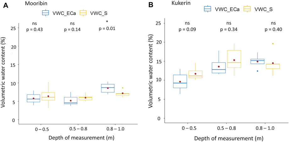
FIGURE 5. Comparison of measured volumetric water content (%) from soil samples (VWC_S) vs. predicted volumetric water content using ERT–EMI calibration curves (VWC_ECa) from inverted EC of the wet season (both taken in August 2019) (A) at Mooribin (B) at Kukerin site. Whiskers indicate the maximum and minimum values at the 95% confidence level, the top and bottom of the box show the 25th and 75th percentiles, the line inside the box is the median value, the dot inside is the mean value, and p values are determined using Wilcoxon test.
Table 3 presents the quality measures of model performance for trained and tested data sets of L. nitens shrub detection. The results obtained had a higher IoU of 93% and 89% for trained and tested data than the recommended PASCAL VOC challenge requirement, which is 50% (Everingham et al., 2010). Visual examples are shown in Figures 6A–C.
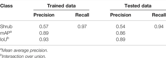
TABLE 3. Shrub count accuracy assessment result.
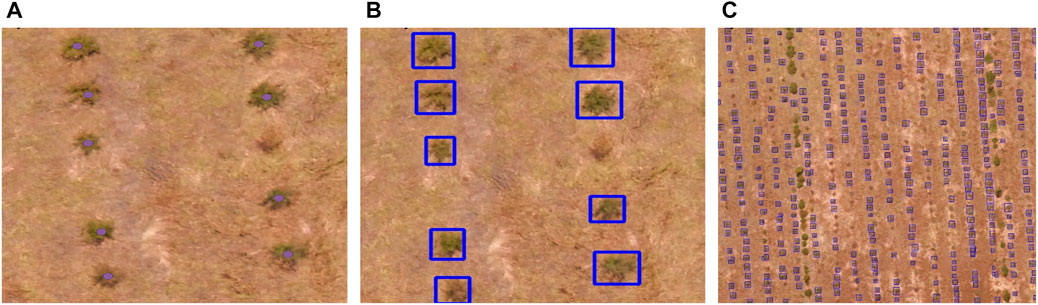
FIGURE 6. Accuracy assessment of UAV imagery and model training example on test set at Mooribin site (A) manually captured shrubs, (B) automated result and (C) sample of automated shrub count results.
UAV-based automated shrub diameter prediction was compared with a manual diameter (cm) taken from three parts of the shrub at Mooribin. Kruskal–Wallis test (Figure 7) showed that shrub prediction using UAV imagery for machine learning was significantly different from the manual shrub diameter measurement for all three measuring areas. Out of all the three manually measured parts of the shrub, measurements from the bottom of the shrub appeared nearest to the machine learning results with an RMSE of 17.1.
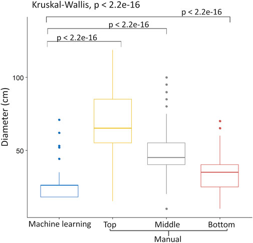
FIGURE 7. Kruskal–Wallis test of manually measured diameter from three heights of Leptospermum plant (top, middle, and bottom) vs. automated canopy diameter estimation using UAV imagery and ML.
Shrub survival and growth patterns estimates from ML were compared from the second inverted EC depth slices (Figures 2B and K) of the dry season survey, which showed the maximum variability at both sites. There were significant differences in estimated L. nitens shrub diameter between areas with different soil inverted EC (Figure 8). In the case of Mooribin, maximum shrub diameter was within the inverted EC range of >6 to 9 mS m−1 (mean 32 cm, SD 7), while the inverted EC ranges of 0–3 and >3 to 6 mS m−1 had shrub diameter of 18–26 cm (Figure 8A). In the case of Kukerin, the inverted EC areas of >12 to 24 and >24 to 36 mS m−1 had a similar average shrub diameter of 31 cm (SD 11) (Figure 8B). However, the range in shrub diameter varied more at >12–24 mS m−1 areas with 18–74 cm than the high inverted EC areas with shrub diameter of 18–55 cm. Furthermore, there was a significant difference in the number of shrubs between these mapped inverted EC areas at both sites, with an overall 77% survival at Mooribin and 82% survival at Kukerin (Table 4).
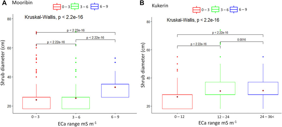
FIGURE 8. Kruskal–Wallis comparison of shrub canopy diameter (cm) (based on UAV-derived ML method) across the sites with three different inverted EC ranges measured at 0.5–0.8 m soil depth (Figures 2B and K) at Mooribin (A) and at Kukerin (B). Whiskers indicate the maximum and minimum values at the 95% confidence level, the top and bottom of the box show the 25th and 75th percentiles, and the dot inside is the mean value.
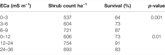
TABLE 4. Shrub survival count based on inverted EC mapped areas.
Figures 9 and 10 present the PCA for the Mooribin and Kukerin sites. The scree plot (Figures 9A and 10A) showed the percentages of variations held by each principal component (PC). The first 3 PCs were retained based on eigenvalues >1 rule (Kaiser et al., 1992), accounting for ∼73% (eigenvalues 7.5, 2.1, and 1.6) and ∼72% (eigenvalues 5.6, 3.4, and 1.8) variation for Mooribin site and Kukerin site, respectively. In Figures 9B and 10B, the projection of the arrows represents the variable loading in their respective PCs. Furthermore, all the soil parameters contributed in the first three PCs; however, the variables contributing above the cut-off line (Figures 9C, 10C) could be considered important in explaining the spatial soil variation influencing L. nitens plantation establishment.
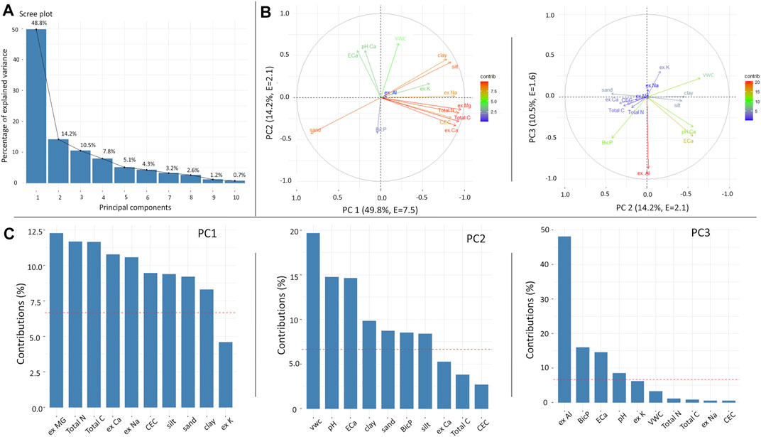
FIGURE 9. Principal component analysis for Mooribin soil parameters showing (A) scree plot, (B) variables highlighted based on their percent contribution in correlation plots, and (C) contribution of variables in selected PCs, where the red line shows the expected average contribution (cut-off). The soil variables included are sand, silt, clay, volumetric water content, pH, CEC, Total N &Total C, ex Mg, ex Na, ex Ca, ex Al, ex K, BicP, and inverted EC from 10 m around each sample.
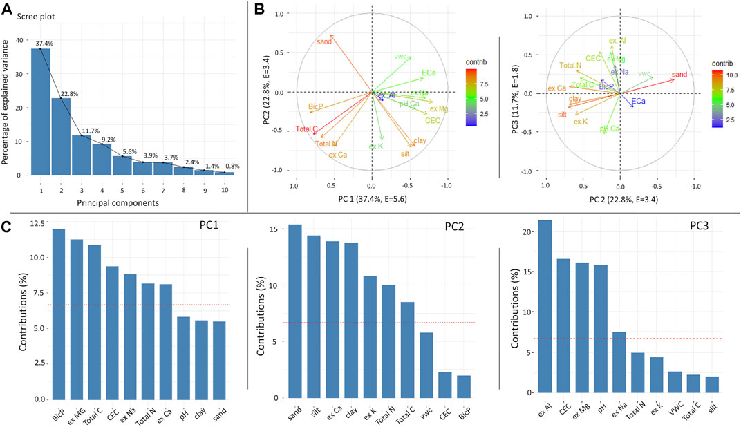
FIGURE 10. Principal component analysis for Kukerin soil parameters showing (A) scree plot, (B) variables highlighted based on their percent contribution in correlation plots, and (C) contribution of variables in selected PCs, where the red line shows the expected average contribution (cut-off). The soil variables included are sand, silt, clay, volumetric water content, pH, CEC, Total N &Total C, ex Mg, ex Na, ex Ca, ex Al, ex K, BicP, and inverted EC from 10 m around each sample.
For Mooribin (Figure 9), the variability explained by PC1 and PC2 was 63%, and inverted EC was strongly correlated to pH > volumetric moisture content > clay and silt and negatively correlated to sand and BicP. There was no correlation between ECa and ex-Mg, Total N, Total C, CEC, ex-Ca, and ex-Na. In PC3 (explaining 10% of the variability), inverted EC was again strongly correlated to pH, followed by silt, clay, and volumetric water content. There was no correlation with the rest of the elements.
For Kukerin (Figure 10), PC1 and PC2 explained a similar amount of variability (62%), and ECa was strongly correlated to volumetric water content > ex-Na > pH, CEC > clay and silt and negatively correlated to ex-Ca, Total N, Total C, BicP, and sand. In PC3 (explaining 12% of the variability), inverted EC had a relatively small contribution but was correlated to volumetric water content, pH, and sand. It showed little or no correlation with silt and clay and a negative correlation with the rest of the parameters.
In this study, a non-invasive EMI survey was used to map soil spatial variability at two sites already planted with L. nitens shrubs. The mapped spatial soil variability was related to newly planted L. nitens survival and growth (shrub canopy diameter) patterns. There was a significant difference in shrub count in the EMI mapped areas at both sites and, overall, a higher shrub count at the variable textured site (Kukerin) as compared to the uniformly sandy site (Mooribin). Areas with higher inverted soil EC were also found to have significantly larger shrub diameters at both the uniform and variable textured site. Therefore, EMI spatial soil mapping can be used to identify areas with different potential for L. nitens plantation establishment.
In areas with low salt concentrations, EMI signal variations generally correspond to differences in soil moisture and soil texture (Brevik and Fenton, 2002). Indeed, the PCA showed inverted EC being inversely correlated to sand and positively correlated to soil moisture. Mooribin was a uniformly deep sandy site with low agronomic value due to water repellence and lower water retention rate (Roper et al., 2015). EMI surveys of this site had lower ECa values, and the ECa values increased from the dry to the wet season. Since soil water was the main variable factor between the seasons, the differences in ECa most likely corresponded to the differences in soil moisture. Our EMI–ERT volumetric moisture prediction values (Figure 5A) were within the range of deep sandy soil moisture rates (Tsoar, 2005). Leptospermum plants performed well in this deep sandy soil, with an overall 75% survival rate ha−1. The 2021 season was relatively wet, and it was also observed that the flowering of shrubs at this site was good, regardless of shrub diameter. EMI survey at variable textured soils of Kukerin had higher ECa values than the uniformly sandy site with overall higher shrub survival (82%) and growth rate. A detailed comparison of shrub survival and growth patterns has shown that sandy loam and loamy textured areas resulted in higher L. nitens survival and growth rate. However, further increase in the clay content did not improve the shrub survival count or diameter (Table 5). This suggests that the performance of Leptospermum plantations at such sites is strongly influenced by soil moisture and is susceptible to drought periods; especially as the water retention of sands is low and soil water availability plays an important role in the successful establishment of native shrubs (Hahs et al., 1999). Moreover, for L. scoparium, studied under controlled conditions, Williams et al. (2014) found that soil composition had little to no impact on the growth and quality of nectar produced. However, water stress was reported to affect the nectar yield (Villarreal and Freeman, 1990; Carroll et al., 2001; Nickless et al., 2017).
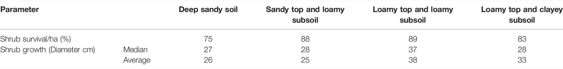
TABLE 5. Leptospermum nitens performance in different soil textures.
Summarized shrub performance with respect to soil texture areas (Table 5) showed that a robust and detailed spatial map of variability could be generated in broad acre sites using EMI surveys. This would effectively improve the soil assessments for planning new plantations and site selection for reforestation or successfully introducing native shrubs in agricultural cropping areas. The EMI survey clearly mapped the different textural classes at the variable site. For example, at Kukerin, the top soil depth slice of 0–0.5 m (2J) had a higher inverted EC toward the top west part of the field during the dry season survey. This was an area of higher clay content and indicated that during the dry soil conditions, soil texture was the most important factor contributing to the ECa values, as found by Abdu et al. (2017) and Doolittle and Brevik (2014).
Generally, medium-textured areas have shown the best shrub establishment rate; however, this textural class is most suitable for agriculture due to their nutrient holding capacity, better aeration, and drainage capacity, as compared to sandy or clayey soils (Salter and Williams, 1965). Nevertheless, heavier textured soil had a survival rate on par with medium-textured soils, so areas with higher clay content and high cost of production for growing crops can be suitable for planting L. nitens. Moreover, L. nitens survival of 75% in deep sandy soil, although the growth rate was lower, can be a good option for utilizing areas with low water retention and repellence rather than cropping.
UAV-based monitoring system helps in reducing the high cost to cover a large area and temporal resolution limitations of satellite sensors (Asner et al., 2009; Kellenberger et al., 2017); nevertheless, for vegetation applications, their 3D point clouds only point to the upper canopy surface and critically miss the sub-canopy structure information (Baltsavias et al., 2008). In this study, the UAV survey for shrub canopy diameter detection was conducted when the shrubs were 2 years old. As such, L. nitens shrubs are not dense when they are young. Therefore, the circles used to model the intensity value of shrub and bare ground might have further contributed to the shrub diameter underestimation. Moreover, there was a gap between the UAV survey and manual diameter measurements of shrubs, which further added to the difference in comparison. It is important to consider the time of UAV imagery survey and ground-truthing as close as possible to get comparable data.
In order to expand the soil-type recommendations for L. nitens, further surveys should be conducted on heavy clay and saline soils, as the current study only considered deep sands and medium-textured soils, which were non-saline. With regards to L. nitens growth on saline soils, Cassaniti et al., 2009 demonstrated relative salt tolerance by L. scoparium plants treated with saline water, where despite high ion concentration in the leaves, plant growth was not affected. However, the quality of nectar produced by their flowers was not studied.
A real-time ECa mapping of the marginal soils showed the impact of spatial soil variability on the establishment and growth patterns of L. nitens plantation. This method was robust and quick to determine the spatial soil variability at both uniform and variable textured sites and in different rainfall seasons. This study demonstrated that the L. nitens cultivations could thrive on marginal agricultural lands. Based on the comprehensive analysis the main conclusions were:
1. L. nitens plantation thrived in a range of soil textures with low fertility; however, there was a significantly larger shrub survival and growth rate in medium and heavier texture areas than in deep sandy areas.
2. Soil moisture can be a limiting factor in shrub survival and growth (shrub canopy diameter) as areas with high inverted EC corresponding to medium texture soil and higher soil moisture retention resulted in higher shrub count and shrub diameter and vice versa. Further studies are required to study the quality and quantity of nectar production by this shrub with respect to EMI mapped areas with different shrub counts and diameter growth.
3. Dry season ECa survey can provide a useful map for marking the soil textural variability, and a wet season map is useful for delineating localized soil management zones, which is particularly useful for intercropping with Leptospermum shrubs.
Data supporting the findings of this study are included in the article/Supplementary Material. Raw data that support the findings of this study are available from the corresponding author, upon reasonable request.
HSS–Main researcher, data acquisition, data analysis, software user, original draft preparation. KFS–Project Supervision, methodology, queries, writing-review and editing. MLS–Project Supervision, methodology and conceptualization review, writing-review.
This research has been generously supported by the Cooperative Research Centre for Honey Bee Products (CRCHBP), Department of Industry, Science, Energy, and Resources Australia (Grant # 20160042).
ML was employed by CRC for Honey Bee Products.
The remaining authors declare that the research was conducted in the absence of any commercial or financial relationships that could be construed as a potential conflict of interest.
All claims expressed in this article are solely those of the authors and do not necessarily represent those of their affiliated organizations, or those of the publisher, the editors, and the reviewers. Any product that may be evaluated in this article, or claim that may be made by its manufacturer, is not guaranteed or endorsed by the publisher.
The first author acknowledges the Australian Government Department of Education and Training that provided her with the Research Training Programme Scholarship. The authors acknowledge Honey for Life group for providing access to the study sites.
The Supplementary Material for this article can be found online at: https://www.frontiersin.org/articles/10.3389/fenvs.2022.883533/full#supplementary-material
Abdu, H., Robinson, D. A., Boettinger, J., and Jones, S. B. (2017). Electromagnetic Induction Mapping at Varied Soil Moisture Reveals Field-Scale Soil Textural Patterns and Gravel Lenses. Front. Agr. Sci. Eng. 4, 135–145. doi:10.15302/J-FASE-2017143
Adams, C. J., Boult, C. H., Deadman, B. J., Farr, J. M., Grainger, M. N. C., Manley-Harris, M., et al. (2008). Isolation by HPLC and Characterisation of the Bioactive Fraction of New Zealand Manuka (Leptospermum scoparium) Honey. Carbohydr. Res. 343, 651–659. doi:10.1016/j.carres.2007.12.011
Adams, C. J., Manley-Harris, M., and Molan, P. C. (2009). The Origin of Methylglyoxal in New Zealand Manuka (Leptospermum scoparium) Honey. Carbohydr. Res. 344, 1050–1053. doi:10.1016/j.carres.2009.03.020
Arshad, M., Li, N., Bella, L. D., and Triantafilis, J. (2020). Field‐scale Digital Soil Mapping of Clay: Combining Different Proximal Sensed Data and Comparing Various Statistical Models. Soil Sci. Soc. Am. J. 84, 314–330. doi:10.1002/saj2.20008
Asner, G. P., Flint Hughes, R., Varga, T. A., Knapp, D. E., and Kennedy-Bowdoin, T. (2009). Environmental and Biotic Controls over Aboveground Biomass throughout a Tropical Rain Forest. Ecosystems 12, 261–278. doi:10.1007/s10021-008-9221-5
Australian Bureau of Statistics (2002). Salinity on Australian Farms 2002, Bulletin 4615. Available at: https://www.abs.gov.au/ausstats/abs@.nsf/mf/4615.0.
Baltsavias, E., Gruen, A., Eisenbeiss, H., Zhang, L., and Waser, L. T. (2008). High‐quality Image Matching and Automated Generation of 3D Tree Models. Int. J. Remote Sens. 29, 1243–1259. doi:10.1080/01431160701736513
Bean, A. R. (1992). The Genus Leptospermum Forst. Et. Forst. F. (Myrtaceae) in Northern Australia and Malesia. Austrobaileya 3, 643–659. doi:10.2307/41738808
Bean, T. (2004). Three New Species of Leptospermum (Myrtaceae) from Queensland and Northern New South Wales. Telopea 10, 831–838.
Beets, P., Kimberley, M., Paul, T., Oliver, G., Pearce, S., and Buswell, J. (2014). The Inventory of Carbon Stocks in New Zealand's Post-1989 Natural Forest for Reporting under the Kyoto Protocol. Forests 5, 2230–2252. doi:10.3390/f5092230
Bennett, D. L., and George, R. J. (1995). Using the EM38 to Measure the Effect of Soil Salinity on Eucalyptus Globulus in South-Western Australia. Agric. Water Manag. 27, 69–85. doi:10.1016/0378-3774(95)91232-V
Bennett, L. (1994). The Expansion of Leptospermum Laevigatum on the Yanakie Isthmus, Wilson's Promontory, under Changes in the Burning and Grazing Regimes. Aust. J. Bot. 42, 555–564. doi:10.1071/BT9940555
Bittelli, M. (2011). Measuring Soil Water Content: A Review. hortte 21, 293–300. doi:10.21273/horttech.21.3.293
BOM (2021). Climate Statistics of Australian Locations. Available at: http://www.bom.gov.au/climate/data/index.shtml.
Brevik, E. C., and Fenton, T. E. (2002). Influence of Soil Water Content, Clay, Temperature, and Carbonate Minerals on Electrical Conductivity Readings Taken with an EM-38. Soil Surv. Horizons 43, 9. doi:10.2136/sh2002.1.0009
Burrell, J. (1965). Ecology ofLeptospermumin Otago. N. Z. J. Bot. 3, 3–16. doi:10.1080/0028825X.1965.10428708
Burrell, J. (1981). Invasion of Coastal Heaths of Victoria by Leptospermum Laevigatum (J. Gaertn.) F. Muell. Aust. J. Bot. 29, 747–764. doi:10.1071/bt9810747
Carroll, A. B., Pallardy, S. G., and Galen, C. (2001). Drought Stress, Plant Water Status, and Floral Trait Expression in Fireweed, Epilobium Angustifolium (Onagraceae). Am. J. Bot. 88, 438–446. doi:10.2307/2657108
Cassaniti, C., Leonardi, C., and Flowers, T. J. (2009). The Effects of Sodium Chloride on Ornamental Shrubs. Sci. Hortic. 122, 586–593. doi:10.1016/j.scienta.2009.06.032
Charron, G., Robichaud-Courteau, T., La Vigne, H., Weintraub, S., Hill, A., Justice, D., et al. (2020). The DeLeaves: a UAV Device for Efficient Tree Canopy Sampling. J. Unmanned Veh. Sys. 8, 245–264. doi:10.1139/juvs-2020-0005
Cokcetin, N. N., Pappalardo, M., Campbell, L. T., Brooks, P., Carter, D. A., Blair, S. E., et al. (2016). The Antibacterial Activity of Australian Leptospermum Honey Correlates with Methylglyoxal Levels. PLoS One 11, e0167780. doi:10.1371/journal.pone.0167780
Cokcetin, N., Williams, S., Blair, S., Carter, D., Brooks, P., and Harry, L. (2019). Active Australian Leptospermum Honey: New Sources and Their Bioactivity. Available at: https://www.agrifutures.com.au/wp-content/uploads/2019/10/19-037.pdf.
Corwin, D. L., and Lesch, S. M. (2013). Protocols and Guidelines for Field-Scale Measurement of Soil Salinity Distribution with ECa-Directed Soil Sampling. Jeeg 18, 1–25. doi:10.2113/JEEG18.1.1
Dainelli, R., Toscano, P., Di Gennaro, S. F., and Matese, A. (2021). Recent Advances in Unmanned Aerial Vehicle Forest Remote Sensing-A Systematic Review. Part I: A General Framework. Forests 12, 327. doi:10.3390/f12030327
Dakak, H., Huang, J., Zouahri, A., Douaik, A., and Triantafilis, J. (2017). Mapping Soil Salinity in 3-dimensions Using an EM38 and EM4Soil Inversion Modelling at the Reconnaissance Scale in Central Morocco. Soil Use Manage 33, 553–567. doi:10.1111/sum.12370
Delefortrie, S., Saey, T., Van De Vijver, E., De Smedt, P., Missiaen, T., Demerre, I., et al. (2014). Frequency Domain Electromagnetic Induction Survey in the Intertidal Zone: Limitations of Low-Induction-Number and Depth of Exploration. J. Appl. Geophys. 100, 14–22. doi:10.1016/j.jappgeo.2013.10.005
D’Emden, F. H., Llewellyn, R. S., and Burton, M. P. (2008). Factors Influencing Adoption of Conservation Tillage in Australian Cropping Regions. Aust. J. Agric. Res. Econ. 52, 169–182. doi:10.1111/j.1467-8489.2008.00409.x
Dixon, D. J., Callow, J. N., Duncan, J. M. A., Setterfield, S. A., and Pauli, N. (2021). Satellite Prediction of Forest Flowering Phenology. Remote Sens. Environ. 255, 112197. doi:10.1016/j.rse.2020.112197
Dodson, J. R., Kershaw, A. P., Arroyo M, F. M. D., and Zedler, P. H. (1995). “Evolution and History of Mediterranean Vegetation Types in Australia,” in Ecology and Biogeography of Mediterranean Ecosystems in Chile, California, and AustraliaEcological Studies (Analysis and Synthesis) (New York, NY: Springer), 21–40. doi:10.1007/978-1-4612-2490-7_2
Doolittle, J. A., and Brevik, E. C. (2014). The Use of Electromagnetic Induction Techniques in Soils Studies. Geoderma 223-225, 33–45. doi:10.1016/j.geoderma.2014.01.027
EMTOMO (2018). EM4Soil: Software for Electromagnetic Tomograph. Available at: https://www.emtomo.com/products/em4soil.
Everingham, M., Van Gool, L., Williams, C. K. I., Winn, J., and Zisserman, A. (2010). The Pascal Visual Object Classes (VOC) Challenge. Int. J. Comput. Vis. 88, 303–338. doi:10.1007/s11263-009-0275-4
Farzamian, M., Autovino, D., Basile, A., De Mascellis, R., Dragonetti, G., Monteiro Santos, F., et al. (2021). Assessing the Dynamics of Soil Salinity with Time-Lapse Inversion of Electromagnetic Data Guided by Hydrological Modelling. Hydrol. Earth Syst. Sci. 25, 1509–1527. doi:10.5194/hess-25-1509-2021
Frischknecht, F. C. (1988). “6. Electromagnetic Physical Scale Modeling,” in Electromagnetic Methods in Applied Geophysics:Theory Investigations in Geophysics (Houston, TX: Society of Exploration Geophysicists), Vol. 1, 364–441. doi:10.1190/1.9781560802631.ch6
Furby, S., Caccetta, P., and Wallace, J. (2010). Salinity Monitoring in Western Australia Using Remotely Sensed and Other Spatial Data. J. Environ. Qual. 39, 16–25. doi:10.2134/jeq2009.0036
George, S. J., Harper, R. J., Hobbs, R. J., and Tibbett, M. (2012). A Sustainable Agricultural Landscape for Australia: A Review of Interlacing Carbon Sequestration, Biodiversity and Salinity Management in Agroforestry Systems. Agric. Ecosyst. Environ. 163, 28–36. doi:10.1016/j.agee.2012.06.022
Griffin, E. A. (1994). Floristic Survey of Remnanat Vegetation in the Dandaragan Area, Western Australia. Western Australia: Department of Agriculture and Food. Perth.
Hageer, Y., Esperón-Rodríguez, M., Baumgartner, J. B., and Beaumont, L. J. (2017). Climate, Soil or Both? Which Variables Are Better Predictors of the Distributions of Australian Shrub Species? PeerJ 5, e3446. doi:10.7717/peerj.3446
Hahs, A., Enright, N. J., and Thomas, I. (1999). Plant Communities, Species Richness and Their Environmental Correlates in the Sandy Heaths of Little Desert National Park, Victoria. Aust. J. Ecol. 24, 249–257. doi:10.1046/j.1442-9993.1999.00969.x
Hanssens, D., Delefortrie, S., Bobe, C., Hermans, T., and De Smedt, P. (2019). Improving the Reliability of Soil EC-Mapping: Robust Apparent Electrical Conductivity (rECa) Estimation in Ground-Based Frequency Domain Electromagnetics. Geoderma 337, 1155–1163. doi:10.1016/j.geoderma.2018.11.030
Harper, R. J., Sochacki, S. J., and McGrath, J. F. (2017). The Development of Reforestation Options for Dryland Farmland in South-Western Australia: a Review. South. For. a J. For. Sci. 79, 185–196. doi:10.2989/20702620.2016.1255417
Harper, R. J., Sochacki, S. J., Smettem, K. R. J., and Robinson, N. (2014). Managing Water in Agricultural Landscapes with Short-Rotation Biomass Plantations. GCB Bioenergy 6, 544–555. doi:10.1111/gcbb.12090
Hedley, C. B., and Yule, I. J. (2009). Soil Water Status Mapping and Two Variable-Rate Irrigation Scenarios. Precis. Agric. 10, 342–355. doi:10.1007/s11119-009-9119-z
Isbell and National Committee on Soil and Terrain (2021). The Australian Soil Classification. Third. CSIRO Publishing. Available at: https://www.soilscienceaustralia.org.au/asc/re/arenosols.htm.
Iuss, W. R. B. (2014). “World Reference Base for Soil Resources 2014, Update 2015 International Soil Classification System for Naming Soils and Creating Legends for Soil Maps,” in World Soil Resources Reports No. 106 (Rome: FAO).
James, I. T., Waine, T. W., Bradley, R. I., Taylor, J. C., and Godwin, R. J. (2003). Determination of Soil Type Boundaries Using Electromagnetic Induction Scanning Techniques. Biosyst. Eng. 86, 421–430. doi:10.1016/j.biosystemseng.2003.09.001
Kaiser, E. A., Mueller, T., Joergensen, R. G., Insam, H., and Heinemeyer, O. (1992). Evaluation of Methods to Estimate the Soil Microbial Biomass and the Relationship with Soil Texture and Organic Matter. Soil Biol. Biochem. 24, 675–683. doi:10.1016/0038-0717(92)90046-Z
Kellenberger, B., Volpi, M., and Tuia, D. (2017). “Fast Animal Detection in UAV Images Using Convolutional Neural Networks,” in 2017 IEEE International Geoscience and Remote Sensing Symposium (Fort Worth: IGARSS), 866–869. doi:10.1109/IGARSS.2017.8127090
Lamb, D. (2014). Large-Scale Forest Restoration. 1st ed. London, UK: Routledge, Taylor & Francis Group. doi:10.4324/9780203071649
Leopold, M., Gupanis-Broadway, C., Baker, A., Hankin, S., and Treble, P. (2021). Time Lapse Electric Resistivity Tomography to Portray Infiltration and Hydrologic Flow Paths from Surface to Cave. J. Hydrology 593, 125810. doi:10.1016/j.jhydrol.2020.125810
Lewinson, E. (2019). outlier_detection_hampel_filter.ipynb. Available at: https://github.com/erykml/medium_articles/blob/master/Machine Learning/outlier_detection_hampel_filter.ipynb.
Lu, J., Carter, D. A., Turnbull, L., Rosendale, D., Hedderley, D., Stephens, J., et al. (2013). The Effect of New Zealand Kanuka, Manuka and Clover Honeys on Bacterial Growth Dynamics and Cellular Morphology Varies According to the Species. PLoS One 8, e55898. doi:10.1371/journal.pone.0055898
Ma, R., McBratney, A., Whelan, B., Minasny, B., and Short, M. (2011). Comparing Temperature Correction Models for Soil Electrical Conductivity Measurement. Precis. Agric. 12, 55–66. doi:10.1007/s11119-009-9156-7
Marden, M., and Phillips, C. (2015). A Review of Research on the Erosion Control Effectiveness of Naturally Reverting Mānuka (Leptospermum scoparium) and Kānuka (Kunzea Ericoides Complex): Implications for Erosion Mitigation of Space-Planted Mānuka on Marginal Hill Country. Report No LC2280. Envirolink Report CO9X1424, Prepared for Hawke’s Bay Regional Council 1562-HBRC210.
Mavric, E., Wittmann, S., Barth, G., and Henle, T. (2008). Identification and Quantification of Methylglyoxal as the Dominant Antibacterial Constituent of Manuka (Leptospermum scoparium)honeys from New Zealand. Mol. Nutr. Food Res. 52, 483–489. doi:10.1002/mnfr.200700282
McKenzie, N., Coughlan, K., and Cresswell, H. (2002). Soil Physical Measurement and Interpretation for Land Evaluation. Melbourne: CSIRO Publishing. Available at: http://hdl.handle.net/102.100.100/198241?index=1.
McKenzie, N., Jacquier, D., Isbell, R., and Brown, K. (2004). Australian Soils and Landscapes: An Illustrated Compendium. Collingwood, Victoria: CSIRO publishing.
McNeill, J. D. (1980). Electromagnetic Terrain Conductivity Measurement at Low Induction Numbers. TN-6. Geonics Limited Mississauga, ON, Canada doi. Available at http://www.geonics.com/pdfs/technicalnotes/tn6.pdf.
Mendham, D. S., White, D. A., Battaglia, M., McGrath, J. F., Short, T. M., Ogden, G. N., et al. (2011). Soil Water Depletion and Replenishment during First- and Early Second-Rotation Eucalyptus Globulus Plantations with Deep Soil Profiles. Agric. For. Meteorology 151, 1568–1579. doi:10.1016/j.agrformet.2011.06.014
Minasny, B., McBratney, A., and Whelan, B. M. (2005). VESPER Version 1.62. Sydney: The University of Sydney, NSW. Australian Centre for Precision Agriculture, McMillan Building A05. Available at: http://www.usyd.edu.au/su/agric/acpa.
Monteiro Santos, F. A. (2004). 1-D Laterally Constrained Inversion of EM34 Profiling Data. J. Appl. Geophys. 56, 123–134. doi:10.1016/j.jappgeo.2004.04.005
Monteiro Santos, F. A., Triantafilis, J., and Bruzgulis, K. (2011). A Spatially Constrained 1D Inversion Algorithm for quasi-3D Conductivity Imaging: Application to DUALEM-421 Data Collected in a Riverine Plain. Geophysics 76, B43–B53. doi:10.1190/1.3537834
Moura, R., Pereira, T., Barros, M. T., Alipio, R., Lima, A. C. S., and Schroeder, M. A. (2018). “Analysis of Frequency-Dependence of Soil Resisitivity: Emphasis at Low Frequencies,” in Conference: International Conference on Grounding and Earthing & 8th International Conference on Lightning Physics and Effects (Pirenopolis, Brazil).
Nicia, P., Bejger, R., Zadrożny, P., and Sterzyńska, M. (2018). The Impact of Restoration Processes on the Selected Soil Properties and Organic Matter Transformation of Mountain Fens under Caltho-Alnetum Community in the Babiogórski National Park in Outer Flysch Carpathians, Poland. J. Soils Sediments 18, 2770–2776. doi:10.1007/s11368-017-1909-8
Nickless, E. M., Anderson, C. W. N., Hamilton, G., Stephens, J. M., and Wargent, J. (2017). Soil Influences on Plant Growth, Floral Density and Nectar Yield in Three Cultivars of Mānuka (Leptospermum scoparium). N. Z. J. Bot. 55, 100–117. doi:10.1080/0028825X.2016.1247732
Pádua, L., Vanko, J., Hruška, J., Adão, T., Sousa, J. J., Peres, E., et al. (2017). UAS, Sensors, and Data Processing in Agroforestry: a Review towards Practical Applications. Int. J. Remote Sens. 38, 2349–2391. doi:10.1080/01431161.2017.1297548
Paz, M. C., Farzamian, M., Paz, A. M., Castanheira, N. L., Gonçalves, M. C., and Monteiro Santos, F. (2020). Assessing Soil Salinity Dynamics Using Time-Lapse Electromagnetic Conductivity Imaging. SOIL 6, 499–511. doi:10.5194/soil-6-499-2020
Pearson, R. K., Neuvo, Y., Astola, J., and Gabbouj, M. (2016). Generalized Hampel Filters. EURASIP J. Adv. Signal Process. 2016, 1–18. doi:10.1186/s13634-016-0383-6
Porter, N. G., and Wilkins, A. L. (1999). Chemical, Physical and Antimicrobial Properties of Essential Oils of Leptospermum scoparium and Kunzea Ericoides. Phytochemistry 50, 407–415. doi:10.1016/s0031-9422(98)00548-2
QGIS.org (2022). QGIS Geographic Information System. Available at: http://www.qgis.org.
R Core Team (2020). R: A Language and Environment for Statistical Computing. Available at: https://www.r-project.org/.
Raparelli, E., and Bajocco, S. (2019). A Bibliometric Analysis on the Use of Unmanned Aerial Vehicles in Agricultural and Forestry Studies. Int. J. Remote Sens. 40, 9070–9083. doi:10.1080/01431161.2019.1569793
Rayment, G. E., and Lyons, D. J. (2011). Soil Chemical Methods: Australasia. Collingwood, VIC: CSIRO publishing.
Redmon, J., Divvala, S., Girshick, R., and Farhadi, A. (2016). You Only Look once: Unified, Real-Time Object Detection. doi:10.1109/CVPR.2016.91
Ronneberger, O., Fischer, P., and Brox, T. (2015). “U-net: Convolutional Networks for Biomedical Image Segmentation,” in Medical Image Computing and Computer-Assisted Intervention – MICCAI 2015. Editors F. A. N. Navab, J. Hornegger, and W. Wells (Springer International Publishing), 234–241. arXiv:1505.04597. doi:10.1007/978-3-319-24574-4_28
Roper, M. M., Davies, S. L., Blackwell, P. S., Hall, D. J. M., Bakker, D. M., Jongepier, R., et al. (2015). Management Options for Water-Repellent Soils in Australian Dryland Agriculture. Soil Res. 53, 786–806. doi:10.1071/SR14330
Salter, P. J., and Williams, J. B. (1965). The Influence of Texture on the Moisture Characteristics of Soils. J. Soil Sci. 16, 310–317. doi:10.1111/j.1365-2389.1965.tb01442.x
Santos, F. A. M., Triantafilis, J., Bruzgulis, K. E., and Roe, J. A. E. (2010). Inversion of Multiconfiguration Electromagnetic (DUALEM-421) Profiling Data Using a One-Dimensional Laterally Constrained Algorithm. Vadose Zo. J. 9, 117–125. doi:10.2136/vzj2009.0088
Sasaki, Y. (2001). Full 3-D Inversion of Electromagnetic Data on PC. J. Appl. Geophys. 46, 45–54. doi:10.1016/S0926-9851(00)00038-0
Sasaki, Y. (1989). Two‐dimensional Joint Inversion of Magnetotelluric and Dipole‐dipole Resistivity Data. Geophysics 54, 254–262. doi:10.1190/1.1442649
Scott, N. A., White, J. D., Townsend, J. A., Whitehead, D., Leathwick, J. R., Hall, G. M., et al. (2000). Carbon and Nitrogen Distribution and Accumulation in a New Zealand Scrubland Ecosystem. Can. J. For. Res. 30, 1246–1255. doi:10.1139/x00-048
Scudiero, E., Skaggs, T. H., and Corwin, D. L. (2017). Simplifying Field-Scale Assessment of Spatiotemporal Changes of Soil Salinity. Sci. Total Environ. 587-588, 273–281. doi:10.1016/j.scitotenv.2017.02.136
Shaukat, H., Flower, K. C., and Leopold, M. (2022). Quasi-3D Mapping of Soil Moisture in Agricultural Fields Using Electrical Conductivity Sensing. Agric. Water Manag. 259, 107246. doi:10.1016/j.agwat.2021.107246
Simons, J., and Bennett, D. (2021). Measuring Soil Salinity. Dep. Prim. Ind. Reg. Dev. Available at: https://www.agric.wa.gov.au/soil-salinity/measuring-soil-salinity (Accessed February 16, 2022).
Stephens, J. M. C., Molan, P. C., and Clarkson, B. D. (2005). A Review ofLeptospermum scoparium(Myrtaceae) in New Zealand. N. Z. J. Bot. 43, 431–449. doi:10.1080/0028825X.2005.9512966
Stirzaker, R. J., Vertessy, R. A., and Sarre, A. (2002). Trees, Water and Salt: An Australian Guide to Using Trees for Healthy Catchments and Productive Farms. Canberra: Joint Venture Agroforestry Program and CSIRO. RIRDC publication number: 01/086.
Thompson, J. (1989). A Revision of the Genus Leptospermum (Myrtaceae). Telopea 3, 301–449449. doi:10.7751/telopea19894902
Thrimawithana, A. H., Jones, D., Hilario, E., Grierson, E., Ngo, H. M., Liachko, I., et al. (2019). A Whole Genome Assembly of Leptospermum scoparium (Myrtaceae) for Mānuka Research. N. Z. J. Crop Hortic. Sci. 47, 233–260. doi:10.1080/01140671.2019.1657911
Triantafilis, J., Laslett, G. M., and McBratney, A. B. (2000). Calibrating an Electromagnetic Induction Instrument to Measure Salinity in Soil under Irrigated Cotton. Soil Sci. Soc. Am. J. 64, 1009–1017. doi:10.2136/sssaj2000.6431009x
Triantafilis, J., Terhune, C. H., and Monteiro Santos, F. A. (2013). An Inversion Approach to Generate Electromagnetic Conductivity Images from Signal Data. Environ. Model. Softw. 43, 88–95. doi:10.1016/j.envsoft.2013.01.012
Tsoar, H. (2005). “Sand Dunes,” in Encyclopedia of Soils in the Environment. Editor D. B. T. Hillel (Oxford: Elsevier), 462–471. doi:10.1016/B0-12-348530-4/00410-0
van Wesenbeeck, I. J., and Kachanoski, R. G. (1988). Spatial and Temporal Distribution of Soil Water in the Tilled Layer under a Corn Crop. Soil Sci. Soc. Am. J. 52, 363–368. doi:10.2136/sssaj1988.03615995005200020011x
Villarreal, A. G., and Freeman, C. E. (1990). Effects of Temperature and Water Stress on Some Floral Nectar Characteristics in Ipomopsis Longiflora (Polemoniaceae) under Controlled Conditions. Bot. Gaz. 151, 5–9. doi:10.1086/337797
Wicaksono, W. A., Jones, E. E., Monk, J., and Ridgway, H. J. (2016). The Bacterial Signature of Leptospermum scoparium (Mānuka) Reveals Core and Accessory Communities with Bioactive Properties. PLoS One 11, e0163717. doi:10.1371/journal.pone.0163717
Williams, S. D., Pappalardo, L., Bishop, J., and Brooks, P. R. (2018). Dihydroxyacetone Production in the Nectar of Australian Leptospermum Is Species Dependent. J. Agric. Food Chem. 66, 11133–11140. doi:10.1021/acs.jafc.8b04363
Keywords: electromagnetic induction (EMI), inversion, volumetric soil moisture, UAV, Leptospermum, electrical resistivity tomography (ERT), dryland, soil mapping
Citation: Shaukat H, Flower KC and Leopold M (2022) Soil Mapping Using Electromagnetic Induction to Assess the Suitability of Land for Growing Leptospermum nitens in Western Australia. Front. Environ. Sci. 10:883533. doi: 10.3389/fenvs.2022.883533
Received: 25 February 2022; Accepted: 17 June 2022;
Published: 19 July 2022.
Edited by:
Niall Patrick Hanan, New Mexico State University, United StatesReviewed by:
Ilan Stavi, Dead Sea and Arava Science Center, IsraelCopyright © 2022 Shaukat, Flower and Leopold. This is an open-access article distributed under the terms of the Creative Commons Attribution License (CC BY). The use, distribution or reproduction in other forums is permitted, provided the original author(s) and the copyright owner(s) are credited and that the original publication in this journal is cited, in accordance with accepted academic practice. No use, distribution or reproduction is permitted which does not comply with these terms.
*Correspondence: Matthias Leopold, bWF0dGhpYXMubGVvcG9sZEB1d2EuZWR1LmF1
Disclaimer: All claims expressed in this article are solely those of the authors and do not necessarily represent those of their affiliated organizations, or those of the publisher, the editors and the reviewers. Any product that may be evaluated in this article or claim that may be made by its manufacturer is not guaranteed or endorsed by the publisher.
Research integrity at Frontiers
Learn more about the work of our research integrity team to safeguard the quality of each article we publish.