 Li Zhang
 Jie Dong
 Lu Zhang1
 Mingsheng Liao
95% of researchers rate our articles as excellent or good
Learn more about the work of our research integrity team to safeguard the quality of each article we publish.
Find out more
ORIGINAL RESEARCH article
Front. Environ. Sci. , 10 March 2022
Sec. Environmental Informatics and Remote Sensing
Volume 10 - 2022 | https://doi.org/10.3389/fenvs.2022.859363
This article is part of the Research Topic Advanced Big SAR Data Analytics and Applications View all 8 articles
Atmospheric propagation delay correction is the key to improving the accuracy of deformation measurement of satellite interferometric synthetic aperture radar (InSAR). The empirical phase-elevation models and external data-based models present uneven performances of atmospheric delay correction for InSAR deformation monitoring. In this study, based on our previous fusion of delays predicted by multiple weather models (FDWM), we propose a new approach of adaptive fusion of multi-source tropospheric delay (AFMTD) estimates derived from multiple models over wide areas, i.e., ERA5, GACOS, WRF, MERRA2, NARR, MODIS, Linear model, and Powerlaw model. The spatially varying scaling algorithm is employed to refine the tropospheric delays predicted by the weather models. Meanwhile, we adopt a multiple-window strategy to cope with the spatially lateral variation of tropospheric delays. The AFMTD not only improves the spatial heterogeneity of tropospheric delay, but also adaptively combines multiple models to achieve a more reliable delay estimation. This AFMTD method is incorporated into the StaMPS-SBAS procedure. We compared the AFMTD with other single models using ENVISAT ASAR and Sentinel-1 datasets over Los Angeles of Southern California. The result of ASAR first demonstrates the effectiveness and reliability of the AFMTD method by referring to the assumed ground truth of simultaneous MERIS observations. The results of Sentinel-1 data show that over 95% of unwrapped interferograms have the minimum root-mean-square values after AFMTD correction for both descending and ascending tracks. The validation against GPS observation presents that the RMSEs of InSAR displacement time series after AFMTD correction decreases at more than 90% of 125 GPS stations. The average reductions of RMSE are 35.79% and 36.28% for descending and ascending data, respectively, and the maximum improvement is more than 70%. Overall, the proposed AFMTD method outperforms any single model for InSAR tropospheric delay correction and provides an open framework to fuse multi-source tropospheric delay estimates.
The atmospheric propagation delay (APD), which stemmed from the refraction of electromagnetic waves when propagating in the nonhomogeneous atmosphere, is a major confusing source in InSAR deformation measurements (Zebker et al., 1997). The APD consists of the ionospheric delay component and tropospheric delay component (Gray et al., 2000). The spatiotemporal variations of ionospheric electron density cause the ionospheric effect. Since the magnitude of ionospheric delay depends on the radar wavelengths, the ionospheric delay in the C-band is about one-sixteenth of that in the L-band (Liang et al., 2019). The ionospheric disturbances rarely affect the C-band SAR at mid-latitude regions.
The tropospheric delays depend on the variations in atmospheric parameters between SAR acquisitions. For example, if the relative humidity changes by 20%, the delay can reach 0.1 m in magnitude, which is sufficient to mask small deformation signals (Zebker et al., 1997). Considering the spatial physical properties of the troposphere delay, it can be divided into vertically stratified delays and turbulence delays (Hanssen, 2001). Many methods were proposed to alleviate the tropospheric effect and can be categorized as follows:
A straightforward estimation solution involves the statistical properties of atmospheric delay and its empirical relationship with local elevations, including stacking (Ferretti et al., 2011), spatial-temporal filtering (Hooper et al., 2007), and phase-elevation models. Apart from linear phase-elevation model that estimates terrain-related tropospheric delays (Cavalié et al., 2007), improved empirical models were proposed, such as multiscale approach (Lin et al., 2010), multiresolution wavelet analysis (Shirzaei and Bürgmann, 2012), iterative linear phase-elevation model (Dong et al., 2019), troposphere height regression (Zebker, 2021), Powerlaw method (Bekaert et al., 2015a) and quad-tree aided joint model (Liang et al., 2018).
The tropospheric delays can also be calculated from external data. There have been several successful cases of estimating tropospheric delays from GNSS zenith delay observations (Onn and Zebker, 2006; Xu et al., 2011; Yu et al., 2018a), weather models of different resolutions (Jolivet et al., 2014; Parker et al., 2015; Murray et al., 2019; Cao et al., 2021), weather forecasting model (Yun et al., 2015; Ulmer and Adam, 2017), and satellite multispectral imagery (Li et al., 2006; Barnhart and Lohman, 2013).
Ignoring the great progress made in estimating tropospheric delays, the aforementioned approaches present unstable behaviors or have inherent defects in certain situations. The empirical phase-based models are difficult to deal with deformation signals correlated with topography. The tropospheric delay estimation from external auxiliary data is not always effective for all scenes. The total zenith delay with short time intervals can be derived from GNSS data, while the spatial distribution of GNSS stations is sparse in most regions of the world. Although the meteorological reanalysis data has the advantage of global or regional coverages, their performances of tropospheric delay corrections differ largely due to the different resolutions in spatiotemporal and various assimilation algorithms. Using space-based multispectral data to obtain wet delays is limited to daylight and cloudless conditions, meanwhile, the errors caused by the time difference between multispectral data and SAR acquisitions vary with the time and region (Li et al., 2009).
In light of the drawbacks of individual tropospheric correction methods, Li et al. (2009) proposed to correct the atmospheric delays by combining MERIS and MODIS. Bekaert et al. (2015b) made a statistical comparison of different atmospheric delay correction methods and suggested that the optimal result can be realized through model fusion. Yu et al. (2018b) developed a tropospheric correction method to integrate weather models and GPS observations. Dong et al. (2019) proposed a fusion model named FDWM that combines tropospheric delays derived from multiple weather models to correct the stratified delay when monitoring single landslides. Shen et al. (2019) proposed the spatially varying scaling (abbreviated as SVS here) algorithm to alleviate the deviation in the estimated tropospheric delay from its truth.
Based on the framework of our previous FDWM fusion model (Dong et al., 2019), we propose a new method to adaptively fuse more tropospheric delays estimated or predicted by the empirical models (Linear and Powerlaw), meteorological reanalysis models (ERA5, GACOS, MERRA2, and NARR), numerical weather forecast model (WRF), and multi-spectral image (MODIS). The new method adopts the SVS algorithm to alleviate the deviation of tropospheric delays calculated by the external weather models. A strategy of multiple windows is used to handle the spatially lateral variation of tropospheric delays for large-scale ground deformation measurements. The tropospheric delay output from the fusion model is imported into the StaMPS-SBAS processing program for correcting the tropospheric delay phases. We first evaluated the performances of individual models and our new fusion model using ENVISAT ASAR data through setting MERIS-derived tropospheric delays as the truth. Then, the applicability of the new fusion model to Sentinel-1 data was explored in terms of unwrapped phases, deformation rates, and displacement time series. Lastly, we ranked the tropospheric delay correction methods and investigated the improvements of our new fusion model to the FDWM and SVS.
The densely populated Los Angeles basin has complex geological structures and many active faults, which makes it often subjected to the complicated subsidence related to tectonic movement and human activities (Watson et al., 2002). This area is adjacent to the Pacific Ocean, and the north is surrounded by mountains. Our study area is marked by white rectangles in Figure 1, with significantly changed topography. There are extensive researches related to atmospheric delay correction conducted here due to the abundant data of weather models and multi-spectral images, as well as dense and continuous GPS observation data.
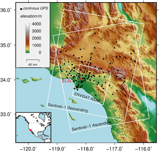
FIGURE 1. The SRTM DEM of the study area as a background map for display. The white rectangles indicate the coverages of descending ENVISAT ASAR data and descending/ascending Sentinel-1 data. The black squares represent the 125 continuous GPS stations. The red star is the location of the InSAR reference point. The red square in the inset represents the location of Southern California.
The SAR data contains one stack of C-band ENVISAT ASAR (ASAR-desc) images and two stacks of C-band Sentinel-1 (S1-desc and S1-asc) images. The former is acquired in stripmap (SM) mode from april 2007 to February 2009 in descending track 170. The latter are acquired in interferometric wide swath (IW) mode from May 2015 to July 2018 in descending track 71 and ascending track 64, respectively. The white rectangles in Figure 1 mark the spatial coverages of the three SAR data stacks. The characteristics of the three SAR datasets are elucidated in Table 1. The Shuttle Radar Topography Mission (SRTM) DEM of approximately 90-m resolution is used for the removal of topographic phases.
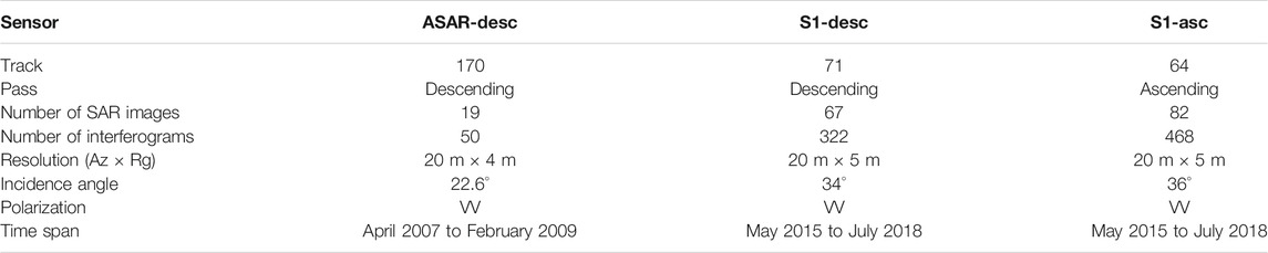
TABLE 1. Parameters of the SAR images.
The Southern California Integrated GPS Network (SCIGN), one of the most densely spaced GPS networks in the world (Hudnut et al., 2001), is constructed to monitor the seismic activities in entire Southern California. Figure 1 shows the locations of 125 permanent GPS stations indicated by black rectangles. The GPS deformation results can be found from the website (http://www.scign.org), which are used to validate the deformation results of InSAR with tropospheric delay corrections.
Four meteorological reanalysis models (ERA5, GACOS, MERRA2, and NARR) and one numerical weather prediction model (WRF) are used to obtain the tropospheric propagation delays. Table 2 lists the parameters of the four meteorological reanalysis models.
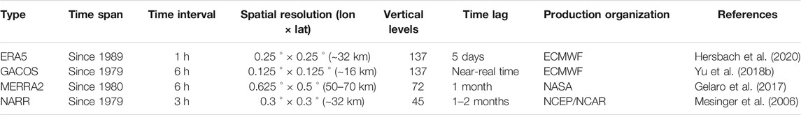
TABLE 2. Informations of the meteorological reanalysis models.
As a new generation of mesoscale numerical weather forecast model, the Weather Research and Forecasting (WRF) model is dedicated to atmospheric simulation and weather forecasting research (Skamarock and Klemp, 2008). The WRF (ARW) 4.0 prediction model developed by National Center for Atmospheric Research (NCAR) is used to simulate atmospheric conditions. The Final Operational Global Analysis (FNL) data of the National Environmental Forecast Center provides initial values and boundary conditions. The experimental simulation runs for 18 h. To enhance the resolution, we set up a three-layer nesting scheme for the WRF simulation experiment, and from the initial grid resolution to the inner nested domain resolution are 27, 9, and 3 km, respectively. The tropospheric delay is estimated using data with a spatial horizontal resolution of 3 km and 37 layers in the vertical direction (1,000–100 hPa).
The Moderate Resolution Imaging Spectroradiometer (MODIS) onboard the Terra and Aqua satellites of NASA is a passive imaging spectrometer including five near-infrared bands that are sensitive to water vapors. The spatial resolution of water vapor products is about 1 km × 1 km, and the water vapor accuracy is claimed to be 5–10%. If the daytime and clear weather are not met, the data accuracy will be worse (Gao and Kaufman, 2003). Given the wet delay estimated by MODIS is overestimated compared with the GPS zenith delay, they need to be corrected before application (Li et al., 2005).
We propose an adaptive fusion of multiple tropospheric delay corrections and incorporate it into the standard StaMPS-SBAS process, with the flowchart shown in Figure 2.
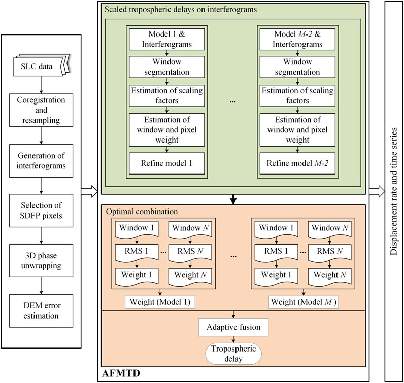
FIGURE 2. Flowchart of the adaptive fusion of multi-source tropospheric delay (AFMTD) estimates.
The ENVISAT ASAR and Sentinel-1 datasets are preprocessed using the commercial GAMMA software (Wegmüller and Werner, 1997). The pre-processing includes SAR image co-registration, interferogram generation, topographic phase removal, and geocoding. We use SRTM DEM to remove the topographic phase.
The interferograms with small baselines are imported into the StaMPS-SBAS time series analysis (Hooper et al., 2007). The amplitude dispersion index (ADI) is used for the selection of coherent candidate points (Ferretti et al., 2001). The slowly-decorrelating filtered phase pixels (SDFP) are further determined by phase stability analysis. The unwrapped phase ∆ϕunw after 3D phase unwrapping (Hooper and Zebker, 2007) contains the following components:
where ∆ϕtopo indicates topographic phase component due to inaccurate external DEM, which is proportional to perpendicular baseline. ∆ϕdefo represents the deformation phase component. ∆ϕatm denotes the atmospheric delay phase, including the ionospheric component and tropospheric component. Since our purpose is to study the tropospheric delay, the ionospheric component is not considered here. ∆ϕorb is the inaccurate orbit phase component, which can be estimated and separated by using a bilinear or biquadratic model. ∆ϕn indicates the phase component caused by the thermal noise, decorrelations, and possible ‘fading signal’ due to multi-looking operation (Ansari et al., 2021).
The proposed adaptive fusion of multiple delay estimates contains two main steps. The first step is to refine the tropospheric phases calculated from the weather models using unwrapped phases. The second step is to perform the adaptively weighting fusion of multi-source tropospheric delays through multiple windows.
The tropospheric delays are estimated from weather models (ERA5, GACOS, MERRA2, NARR, and WRF), spectrometer observation products (MODIS), and empirical models (Linear and Powerlaw) using the TRAIN software (Bekaert et al., 2015b).
When predicting tropospheric phases using the weather models, the interpolations in space and time generally result in biased tropospheric delay estimation. We introduce the SVS algorithm to alleviate the biases and to make it closer to the correct value of tropospheric delay for large-scale areas (Shen et al., 2019). The SVS algorithm is repeated simply here to keep the methodology intact.
We divide each interferogram into N regular non-overlapping windows. The window size is set as 50 km here. The relationship between unwrapped phase ∆ϕunw and tropospheric delay phase ∆ϕtropo predicted from weather model data in a single window is taken as linear:
where Ki and Ci indicate the scaling factor and constant offset at window i, respectively.
The scaling factors for each window are smoothed through a weighting strategy, which is carried out as follows:
(1) The first step is to weigh each window through a signal-to-noise ratio. Var(ϕtropo(i)) represents the variance of tropospheric delay phase in window i, i.e. signal. Var(ϕres(i)) is the variance of residual phase, i.e. noise. The residual phase equals to unwrapped phase subtracted by the tropospheric delay phase. The signal-to-noise ratio of tropospheric delay phase in window i is expressed as:
(2) The second step is to weigh each pixel. The weight of each pixel is calculated according to the distance using a two-dimensional Gaussian smoothing function:
where (xi, yi) represents the central coordinate of window i, the coordinates of each pixel are denoted by (x,y). σd is the standard deviation width, i.e. the Gaussian filter width. A Gaussian filter width of 70 km is used here.
(3) The last step is to combine the weights in steps (1) and (2) to derive the smoothed scaling factor K (x,y) for every pixel:
The smoothed scaling factor K (x,y) is used to replace the one in Eq. 2 to obtain the scaled tropospheric delay phase for each weather model.
The tropospheric delay phases predicted from the weather model data and spectrometer observation products are refined in Scaled tropospheric phases estimated by weather model data. Since these methods present unstable performances for different SAR data at different regions, Dong et al. (2019) proposed an optimal weighting fusion of multiple tropospheric delays using a single weight. However, in the case of wide coverages (larger than tens of kilometers), the single weight is not sufficient to describe the spatially lateral variation of tropospheric delays for the entire scene (Bekaert et al., 2015a).
We divide the large scene into N windows using the same window size and layout as described in Scaled tropospheric phases estimated by weather model data and derive weights for each window. The final tropospheric delay phase ∆ϕtropo (x,y) on pixel (x, y) can be obtained through weighting fusion of M tropospheric delay corrections:
where ∆ϕjtropo (x,y) denotes the tropospheric delay phase estimated by correction model j with corresponding weight wj (x, y). The weight is calculated from the root-mean-square (RMS) value
where the p is set as two here. If the RMS value
In this section, the effectiveness of AFMTD method was first evaluated on ENVISAT ASAR data using the integrated precipitable water vapor from MERIS. We then analyzed the applicability of AFMTD method to correct tropospheric delays for frequently-used Sentinel-1 data, which is validated by the GPS measurements.
The MERIS sensor mounted on the ENVISAT satellite is synchronized with ASAR acquisitions and has two modes of full and reduced resolutions. Previous studies have demonstrated the advantages of MERIS water vapor products for mitigating atmospheric effects from ASAR data under cloud-free conditions (Xu et al., 2010). Compared with GPS observations, the standard deviation of MERIS water vapor products is 1.1 mm (Li et al., 2006).
We used MERIS-derived tropospheric delays as truth values to evaluate the effects of tropospheric delay corrections. Since the hydrostatic delay component cannot be ignored for total tropospheric delay (Jolivet et al., 2014), we obtained the MERIS tropospheric delay by adding the mean value of hydrostatic delays derived from ERA5, WRF, MERRA2, and NARR.
A total of 50 interferograms were generated from 19 ENVISAT ASAR images. The maximum temporal and normal baselines were set as 150 days and 450 m to exclude observations of strong temporal-spatial decorrelations, respectively. Figure 3A shows the original unwrapped phase of one interferogram with the primary and secondary images acquired on 7 June 2008 and 16 August 2008, respectively. The temporal and normal baselines are 70 days and 25 m, respectively. The MERIS-estimated delay was taken as the reference to evaluate other models (Figure 3B). The MODIS water vapor products met the 80% cloud-free conditions on the two SAR acquisition dates. Figures 3C–J represents the tropospheric delays obtained by ERA5, GACOS, WRF, MERRA2, NARR, MODIS, Linear, and Powerlaw, respectively. The root mean square errors (RMSEs) of the difference between the MERIS-derived delay and the others are labeled in corresponding sub-plots. The RMSEs for NARR and Powerlaw exceed 5 rad. The other models have RMSEs ranging from 2 rad to 3.5 rad. The NARR may fail to model the atmospheric effect due to its low spatial resolution and the employed assimilation algorithm. Only one sounding ball data used to estimate the Powerlaw coefficient is insufficient to represent the spatially varying atmosphere and results in a deviation in the estimated scale coefficient for the Powerlaw method (Bekaert et al., 2015b). The AFMTD method fused the tropospheric delay phases in Figures 3C–J and has the minimum RMSE value of 1.94 rad (Figure 3K), outperforming all other models. Since the MODIS water vapor products are restricted to daytime and cloudless conditions, we tested the effectiveness of AFMTD without MODIS. The AFMTD without MODIS still has the minimum RMSE value of 2.19 rad (Figure 3M).
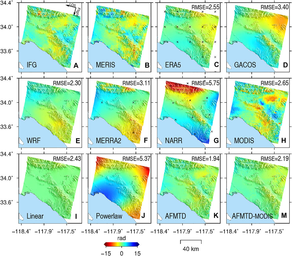
FIGURE 3. Tropospheric delay correction for interferogram 20080607_20080816. (A) Original unwrapped phase and the tropospheric delay phases derived from (B) MERIS, (C) ERA5, (D) GACOS, (E) WRF, (F) MERRA2, (G) NARR, (H) MODIS, (I) Linear (J) Powerlaw (K) AFMTD, and (M) AFMTD without MODIS. The RMSEs of the difference between the MERIS-derived delay and the others are labeled in corresponding sub-plots.
The MERIS data with 80% cloudless observations are available for 25 out of the 50 interferograms. Among these 25 interferograms, the AFMTD method has 12 interferograms with minimum RMSE values. Furthermore, a statistical evaluation on all 50 unwrapped phases was performed. Figure 4 shows the RMS values of unwrapped phases after tropospheric delay correction. In total, 40 out of 50 interferograms have the minimum RMS values after AFMTD correction. Therefore, the AFMTD has its superiority in correcting tropospheric delays over any individual models.
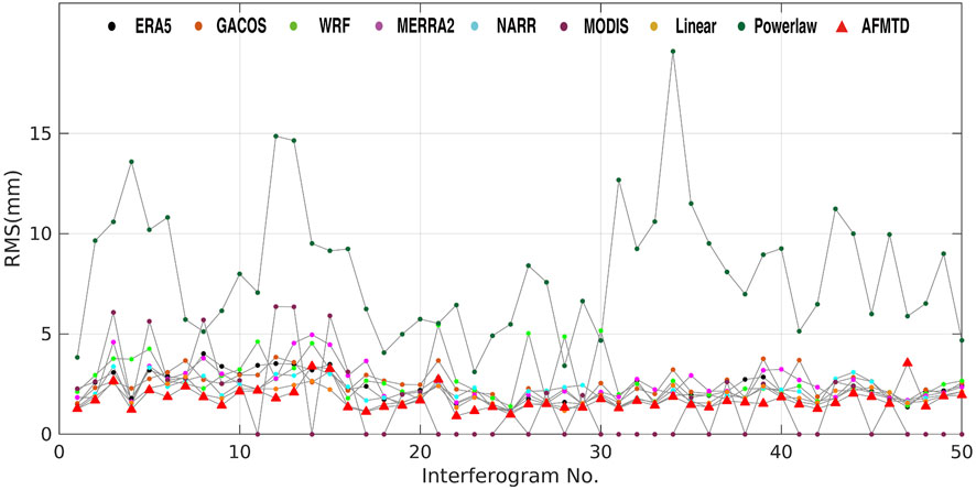
FIGURE 4. The RMS values of ASAR unwrapped phases corrected by tropospheric delays estimated by ERA5, GACOS, WRF, MERRA2, NARR, MODIS, Linear, Powerlaw, and AFMTD.
Since the massive archived Sentinel-1 data largely promotes the wide applications of InSAR technology in various fields, it is essential to evaluate the applicability of the AFMTD method to Sentinel-1 data. In terms of image combination of S1-desc and S1-asc, seven secondary scenes were connected to the primary scene on both sides, with the limitation of the normal baselines and temporal were lower than 200 m and 90 days, respectively. We adopted a multi-looking operation with 24 looks and six looks in range and azimuth, respectively. The red star in Figure 1 marks the spatial reference point.
We made a statistical analysis of the RMS values of residual unwrapped phases corrected by all tropospheric delay correction methods to assess their performance. In terms of S1-desc data (Figure 5), the mean RMS values for ERA5, GACOS, WRF, MERRA2, NARR, MODIS, Linear, and Powerlaw range from 3.24 rad to 10.42 rad, and the STD of RMS values range from 1.02 rad to 5.21 rad. The AFMTD method has 320 minimum RMS values out of all 322 interferograms. The mean and STD of RMS values are 2.15 rad and 0.56 rad, respectively. Both the mean and STD declined by more than 30% compared to any single model.
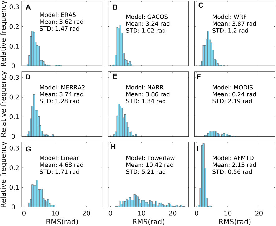
FIGURE 5. The statistical histograms of the RMS of residual unwrapped phases for S1-desc data corrected by (A) ERA5, (B) GACOS, (C) WRF, (D) MERRA2, (E) NARR, (F) MODIS, (G) Linear, (H) Powerlaw, and (I) AFMTD. The corresponding mean and STD values are labeled in each sub-plot.
The statistical histograms of RMS values on the S1-asc data in the supplementary material (Supplementary Figure S1). There are 450 out of 468 interferograms having the minimum RMS values after AFMTD correction. The mean and STD are 3.09 rad and 0.98 rad, respectively, which decreased by more than 25% compared to any single model.
The STD of the S1-asc RMS values is larger than the S1-desc, indicating stronger fluctuation of the former. Besides, the S1-asc RMS presents an approximately periodic fluctuation (Supplementary Figure S2), with the maximum and minimum values appearing in summer and winter, respectively. The acquisition time of S1-asc data is 01:50 UTC, corresponding to the local time of 17:50 at dusk. The S1-desc data is obtained at 13:52 UTC, corresponding to the local time of 05:52 a.m. at dawn. The stronger variation of water vapor at dusk than at dawn may cause the discrepancy between S1-desc and S1-asc data.
We evaluate the effects of tropospheric delay correction on the InSAR annual mean linear deformation rate. The original deformation rates of S1-desc data and the ones corrected using ERA5, GACOS, WRF, MERRA2, NARR, MODIS, Linear, Powerlaw, and AFMTD are plotted in Figure 6. There are several active geological faults in the study area, among which the most active San Andreas Fault (SAF) is the boundary between plates, driving much of the geological disasters (Tong et al., 2013). The deformation rate reflects the crustal movement around the SAF fault and the subsidence caused by non-tectonic activities, such as the subsurface fluid extraction.
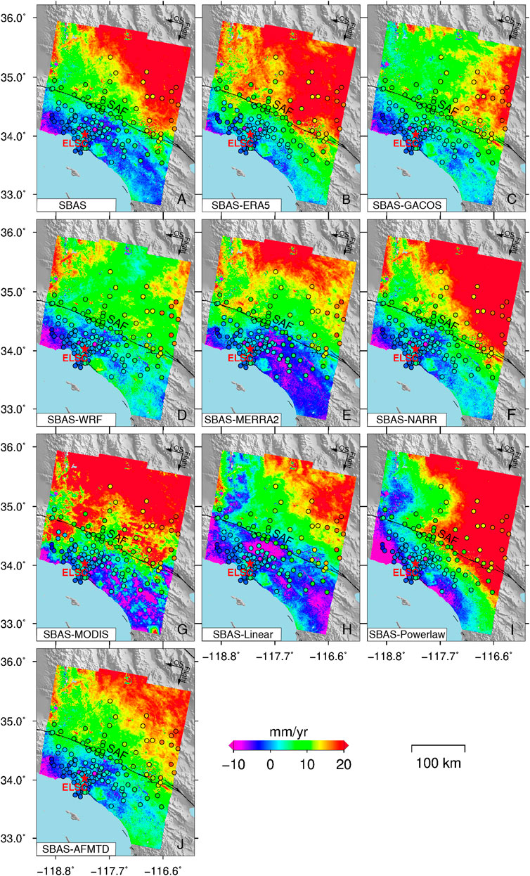
FIGURE 6. The LOS annual mean deformation rate of S1-desc data. The original deformation rate (A) and the deformation rate using (B) ERA5, (C) GACOS, (D) WRF, (E) MERRA2, (F) NARR, (G) MODIS, (H) Linear, (I) Powerlaw, and (J) AFMTD correction. The 125 GPS stations (represented by circles) in this region were colored with the deformation rate calculated from GPS observations along the LOS direction. The red star is the location of the InSAR reference point.
The effectiveness of AFMTD method for InSAR deformation was validated by continuous GPS observations. Excluding the reference station, we collected the observations at 125 GPS stations from 2015 to 2018 from the website of http://www.scign.org. The three-dimensional GPS time series were projected onto the Sentinel-1 LOS direction (Hanssen, 2001). We averaged the InSAR deformation rate within a 300 m radius at each GPS station and compared them with the GPS observations.
We estimated the GPS deformation rate along the SAR LOS direction on the 125 GPS stations by the least square method, as shown in Figure 6. The InSAR deformation rate corrected by AFMTD method shows the best consistency with GPS in terms of both pattern and magnitude. Figure 7 shows the scatterplots of InSAR and GPS deformation rates on 125 GPS stations, as well as the RMSE and R2 provided in each sub-plot. The AFMTD method has a minimum RMSE of 3.25 mm/yr. The RMSEs of other models vary from 3.29 mm/yr to 7.92 mm/yr.
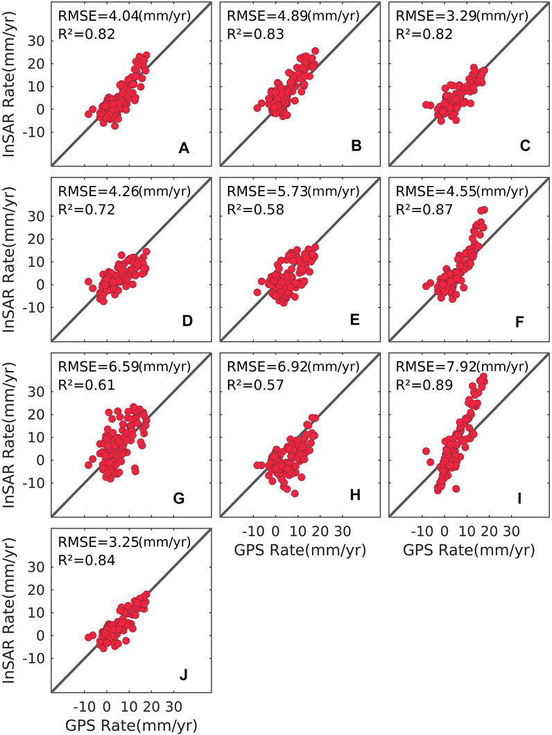
FIGURE 7. Comparison between the GPS observations and (A) the original deformation rate of S1-desc data and the ones using (B) ERA5, (C) GACOS, (D) WRF, (E) MERRA2, (F) NARR, (G) MODIS, (H) linear, (I) powerlaw, and (J) AFMTD corrections on 125 GPS sites. The corresponding RMSE values are labeled in each sub-plot.
Although the NARR and Powerlaw methods have high R2 of 0.87 and 0.89, there are large discrepancies between their deformation rates and GPS observations as shown in Figures 7F,I. The ERA5 and NARR overestimated the deformation rate in the north side of SAF fault (Figures 6B,F and Figures 7B,F), while the WRF and MERRA2 underestimated the deformation rate (Figures 6D,E and Figures 7D,E). These may be caused by different assimilation algorithms and spatio-temporal resolutions of each weather model data. Different from WRF and MERRA2, the rate underestimation by the linear method is located in mountainous areas (Figure 6H and Figure 7H). The deformation rate discrepancy between GPS and MODIS correction is caused by the inconsistent acquisition time of MODIS data with SAR data (Figure 6G and Figure 7G). The deviation of deformation rate corrected by Powerlaw method from GPS may result from the inaccurate powerlaw coefficient estimation (Figure 6I and Figure 7I).
The original deformation rate and the ones corrected by every single model and AFMTD for the S1-asc data and the scatterplots between InSAR and GPS are put in the supplementary material (Supplementary Figure S3 and Supplementary Figure S4). Similar to the S1-desc result, the S1-asc deformation rate after AFMTD correction is most accurate relative to the GPS observations.
We calculated the RMSE of InSAR displacement time series with and without tropospheric delay corrections relative to the GPS observations. 123 out of 125 GPS stations are presenting reduced RMSE values for the S1-desc (Figure 8A). Figure 8B shows the improvement of RMSE corresponding to each GPS site. The positive and negative values indicate decreased and increased RMSE after AFMTD correction. The AFMTD method achieved an average RMSE reduction of 35.79%, and the biggest improvement is more than 75%.
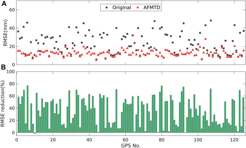
FIGURE 8. Statistical analysis of RMSE for S1-desc data. (A) The RMSE of the InSAR displacement time series without and with AFMTD correction. (B) The reduction percentage of RMSE after AFMTD correction.
We compared the displacement time series between InSAR and GPS observations on 12 GPS stations (black squares in Figures 9A,B). Compared with the original InSAR displacement time series, the displacement time series after AFMTD correction becomes much closer to the GPS observations, which can also be confirmed by the RMSE marked in each sub-plot (Figure 9C).
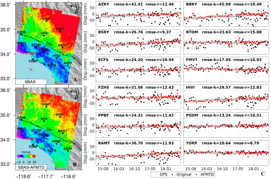
FIGURE 9. Validation of S1-desc InSAR displacement time series against GPS observations (gray cross) on 12 GPS stations marked by black squares in (A) the original deformation rate and (B) the one corrected by AFMTD. (C) The InSAR time series without (black dots, rmse-k) and with AFMTD correction (red dots, rmse-r).
For the S1-asc data, 116 out of 125 GPS stations are showing decreased RMSE after AFMTD correction (Supplementary Figure S5). The average and maximum improvements of RMSE values are 36.28% and 73.16%, respectively. The comparison of displacement time series on 12 GPS stations for S1-asc data is shown in Supplementary Figure S6. The InSAR time series corrected by AFMTD shows good agreement with GPS observations, especially, the seasonal variation of deformation time series was effectively reduced on sites BSRY and RAMT after the AFMTD correction. The InSAR time series fluctuations of S1-asc data are greater than the S1-desc data. This may be explained by the fact that the periodic phenomenon of tropospheric delay in the S1-asc acquisition time is more obvious, which can be demonstrated using the phenomenon in Supplementary Figure S2.
The above experimental results demonstrate the advantages of AFMTD in InSAR tropospheric delay correction. We first ranked the performance of all the used tropospheric delay corrections by comparing them against the GPS observations. Then, we compared the proposed AFMTD with our previous fusion model (FDWM) (Dong et al., 2019) and the SVS method (Shen et al., 2019). Lastly, some future improvements were discussed.
We computed RMSEs of InSAR time series corrected by different tropospheric delays for the 125 GPS stations relative to the GPS measurements. In Figures 10A,B, we showed the number of minimum RMSE values for the eight single models and the AFMTD method for S1-desc and S1-asc data, respectively. The AFMTD method has the largest numbers of minimum RMSE for both the S1-desc of 92 stations and the S1-asc of 98 stations. The GACOS takes second place with 12 and nine stations for the S1-desc and S1-asc, respectively. Other models have less than eight stations with minimum RMSE for both SAR tracks.
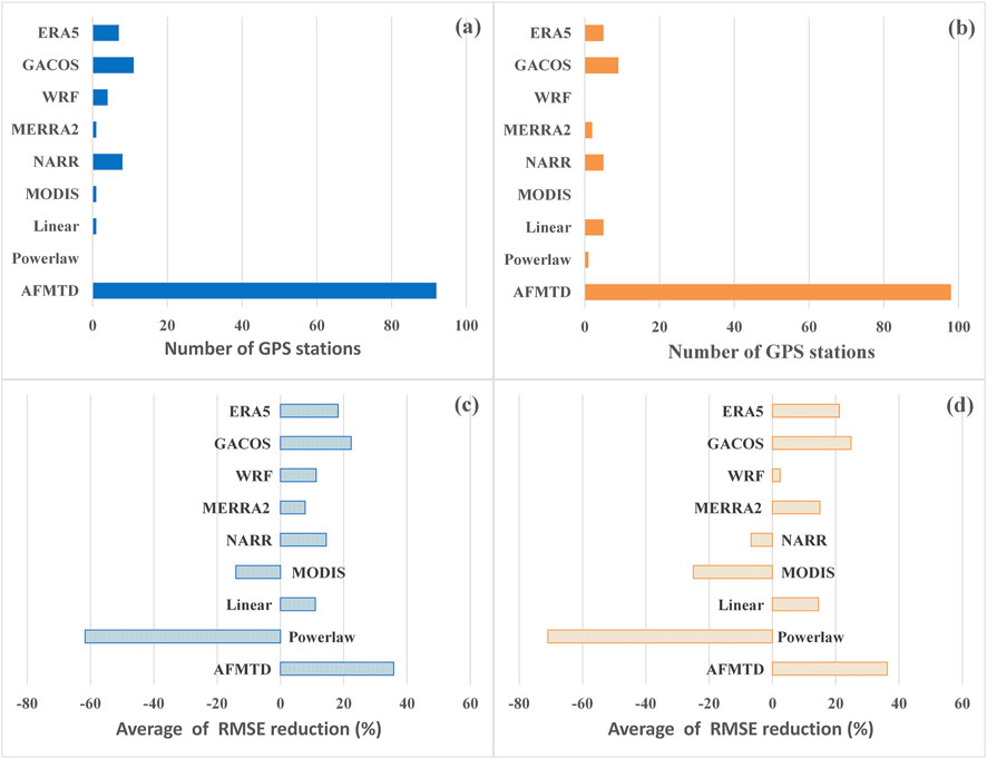
FIGURE 10. The performance evaluation of tropospheric delay corrections. The number of minimum RMSE for (A) S1-desc and (B) S1-asc data. The average improvement of RMSE for (C) S1-desc and (D) S1-asc data. Comparison of AFMTD with FDWM and SVS.
In addition, we calculated the average RMSE improvement of displacement time series on 125 GPS stations after tropospheric delay corrections for the S1-desc and S1-asc (Figures 10C,D). The AFMTD improves 35.79% and 36.28% for the S1-desc and S1-asc, respectively. The GACOS has just over 20% improvement for both tracks. The ERA5 has a slightly worse effect than GACOS. The improvements for WRF, MERRA2, NARR, and Linear are small.
On the contrary, the MODIS and Powerlaw have negative values for both tracks, indicating the degeneration of time series after their corrections. The MODIS water vapor product with high spatial resolution did not achieve the result we expect. In addition to the overestimation of MODIS itself, the reason for this phenomenon is that MODIS products are restricted to be acquired under daytime and cloudless conditions, which cannot be applied to all SAR images. More importantly, the large time gap of several hours between MODIS and Sentinel-1 makes it impossible to capture the true water vapor during SAR image acquisitions. For Powerlaw, the two input coefficients are estimated from one balloon sounding data, which may cause the deviation of tropospheric delay estimation from the true value. The wrong separation of the bands insensitive to deformation may be another factor that causes distortion signal to be confused with troposphere delay correction. The selection of window size also affects the Powerlaw correction.
Overall, considering the number of minimum RMSEs and the average improvement, our AFMTD method takes first place, following by the GACOS. The ERA5 ranks third. The performances of other models are limited and unstable.
Our AFMTD method enriches the framework of the FDWM fusion model proposed by Dong et al. (2019). The FDWM method is only applicable to local-scale landslides. However, the AFMTD adopts the strategy of multiple windows to achieve tropospheric delays correction for large-scale ground deformation measurements. Furthermore, the SVS algorithm is integrated into the AFMTD to alleviate the deviation of tropospheric phases estimated by the external weather models (Shen et al., 2019). We evaluated the improvements of AFMTD relative to FDWM and SVS.
Here, the S1-desc and S1-asc data use the FDWM method to correct the tropospheric delay phase. Only one weight over the whole scene was used for each model for the final fusion. We calculated the mean and STD of the S1-desc and S1-asc RMS for AFMTD and FDWM, as shown in Figures 11A,B. The mean and STD of the S1-desc data are 2.15 rad and 0.56 rad for AFMTD, respectively. The FDWM has slightly poor performance with the mean and STD of 3.17 rad and 1.03 rad, respectively. The mean RMS of the S1-asc data is 3.09 rad and 4.10 rad for AFMTD and FDWM, respectively, as well as the STD of 0.98 rad and 1.46 rad.
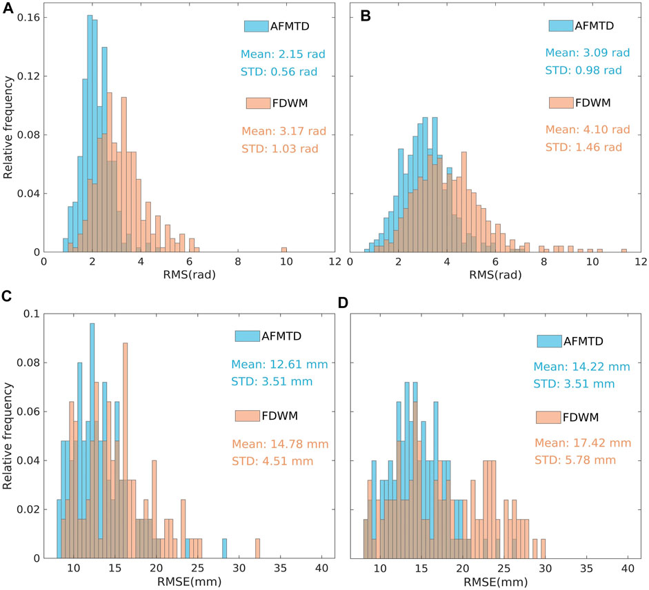
FIGURE 11. The RMS values of residual unwrapped phases using FDWM and AFMTD corrections for S1-desc (A) and S1-asc (B) data. The RMSE between GPS time series and the InSAR time series with FDWM and AFMTD correction for S1-desc (C) and S1-asc (D) data, respectively. The Mean and STD are marked in corresponding sub-plots.
We also compared the RMSEs between the GPS displacements time series and the InSAR ones with FDWM and AFMTD correction on the 125 GPS stations. The mean of S1-desc RMSEs are 14.78 mm and 12.61 mm for FDWM and AFMTD, respectively, and the STD are 4.51 mm and 3.51 mm (Figure 11C). The S1-asc results are similar to those of S1-desc data (Figure 11D). Therefore, the AFMTD performs better than the FDWM in both unwrapped phases and InSAR time series.
The tropospheric delays predicted from the weather model can be refined by the SVS algorithm. We conducted a statistical comparison between SVS-refined tropospheric corrections and the AFMTD for both S1-desc and S1-asc data (Figure 12). In terms of the S1-desc data, the AFMTD method has 219 minimum RMS values out of the 322 interferograms. The number of minimum RMS values corrected by the refined GACOS (GACOS_svs) is 34, ranking second, followed by ERA5_svs with 29 minimum RMS values. The number of minimum RMS values of other models ranges from zero to 16. The S1-asc has a similar phenomenon. After using AFMTD correction, 247 out of the 468 interferograms have the minimum RMS. The number of minimum RMS are 93, 90, 20, 11, 7, and 0 for GACOS_svs, ERA5_svs, WRF_svs, MERRA2_svs, NARR_svs, MODIS_svs, respectively. Therefore, the AFMTD model does better than the SVS-refined tropospheric delay corrections.
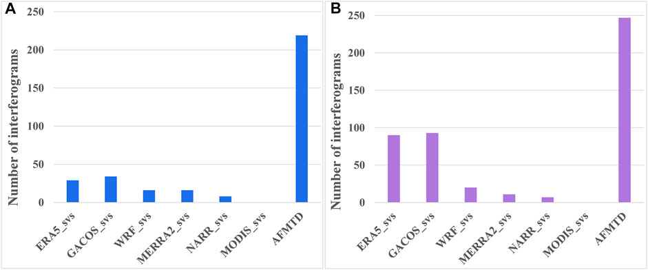
FIGURE 12. Statistical comparison between SVS-refined tropospheric corrections and AFMTD for (A) S1-desc and (B) S1-asc data, respectively.
The most important part of the AFMTD model fusion is to optimally weigh each model. The weight of each model is determined by the RMS of residual unwrapped phase corrected by tropospheric delays. The study area includes a large-scale tectonic deformation caused by a strike-slip fault (SAF). After using the SVS method to refine the weather model, the tectonic deformation will be underestimated. A strategy of subtracting the estimated deformation before conducting the SVS algorithm can partly alleviate the underestimation of large-scale tectonic deformation. Other metrics, for example, the spatial structure functions (Murray et al., 2019), can be employed to calculate the weights of each model to maximize the accuracy of the tropospheric delay estimation.
Another key to the AFMTD method is the window size and Gaussian filter width when smoothing the scaling factors of each window. We used empirical values in this study. Although the regular window can reflect the spatially lateral variation of troposphere delays, we expect that the adaptive window can be closer to the troposphere delays. Using GPS observations to estimate the true value of water vapor to define the Gaussian width is the most accurate way. However, in the future, we expect to obtain the empirical value of Gaussian filter widths through many statistical calculations when no true values of water vapor are available.
The InSAR displacement time series becomes gentle after AFMTD correction, but small fluctuations still exist. This may be owing to the coarse spatiotemporal resolution of the weather model (ranging from few to tens of kilometers), which cannot effectively estimate the turbulence effects of small and medium scales. The remaining small fluctuations can be optionally corrected by spatio-temporal filtering.
This study proposed an adaptive fusion of multi-source tropospheric delay (AFMTD) to estimate the optimal InSAR tropospheric delay. The AFMTD can mitigate the uneven performance of single tropospheric delay models by assigning weights to different tropospheric delay estimates. The SVS algorithm improves the tropospheric delay estimates from weather model data. The multiple-window strategy can cope with the lateral variation of tropospheric delays over wide areas. We summarized the main conclusions as follows.
First, the MERIS-derived truth value demonstrated the advantage of AFMTD over any single model to correct tropospheric delays for individual interferograms. The mean and STD of RMS values of residual unwrapped phases after AFMTD correction are more than 30% and 25% lower than any single model for both S1-desc and S1-asc data, respectively.
Second, the validation of AFMTD-corrected InSAR results against GPS observations shows that more than 90% of 125 GPS stations have reduced RMSE of displacement time series. The average reductions of RMSE are 35.79% and 36.28% for S1-desc and S1-asc, respectively, and the maximum improvement is more than 70%.
Third, the AFMTD model extends our previous FDWM model to apply for large-scale InSAR tropospheric delay correction and outperforms the SVS-refined tropospheric delay estimates.
The AFMTD provides an open framework to fuse multiple tropospheric delays, which is easy to take in new tropospheric delays. Future work will consider adaptive window segmentation according to application scenarios. Meanwhile, other weighting methods can be adopted to deal with different types of tropospheric correction methods to maximize the contribution of each model.
The original contributions presented in the study are included in the article/Supplementary Material, further inquiries can be directed to the corresponding author.
LZ: Conceptualization, Methodology, Visualization, Formal analysis, Writing—original draft. JD: Formal analysis, Data pre-processing, Writing—review and editing. LZ: Writing—review, Supervision. YW: Methodology. WT: Data curation, Validation. ML: Supervision.
This work was financially supported by the National Natural Science Foundation of China (grant numbers 41904001 and 41774006), the Natural Science Foundation of Hubei Provincial (grant number 2019CFB141), the China Postdoctoral Science Foundation (grant number 2018M640733), and the National Postdoctoral Program for Innovative Talents (grant number BX20180220).
The authors declare that the research was conducted in the absence of any commercial or financial relationships that could be construed as a potential conflict of interest.
All claims expressed in this article are solely those of the authors and do not necessarily represent those of their affiliated organizations, or those of the publisher, the editors, and the reviewers. Any product that may be evaluated in this article, or claim that may be made by its manufacturer, is not guaranteed or endorsed by the publisher.
We thank European Space Agency (ESA) for providing the ENVISAT and Sentinel-1 data through the ESA-MOST Dragon five Program (id 59332). We thank Andrew Hooper and Bekaert David for sharing the StaMPS and TRAIN programs, respectively. We thank the National Aeronautics and Space Administration (NASA) for providing the SRTM DEM. We thank European Centre for Medium Range Weather Forecasts (ECMWF) for providing the ERA5 data. Thanks for the GACOS products were provided by Newcastle University, and WRF data provided by NCAR/UCAR, and the MERRA2 data provided by NASA/GMAO, and the NARR data provided by NCEP/NCAR, and the MODIS product provided by NASA Earth Data. We thank UNA VCO Data Center to provide the GPS data. We thank the Department of Atmospheric Science of the University of Wyoming for providing us the sounding data. We thank P. Wessel, W. H. F. Smith, R. Scharroo, J. Luis and F. Wobbe from the University of Hawaii for providing the General Mapping Tools (GMT).
The Supplementary Material for this article can be found online at: https://www.frontiersin.org/articles/10.3389/fenvs.2022.859363/full#supplementary-material
Ansari, H., De Zan, F., and Parizzi, A. (2021). Study of Systematic Bias in Measuring Surface Deformation with SAR Interferometry. IEEE Trans. Geosci. Remote Sensing 59, 1285–1301. doi:10.1109/TGRS.2020.3003421
Barnhart, W. D., and Lohman, R. B. (2013). Characterizing and Estimating Noise in InSAR and InSAR Time Series with MODIS. Geochem. Geophys. Geosyst. 14, 4121–4132. doi:10.1002/ggge.20258
Bekaert, D. P. S., Hooper, A., and Wright, T. J. (2015a). A Spatially Variable Power Law Tropospheric Correction Technique for InSAR Data. J. Geophys. Res. Solid Earth 120, 1345–1356. doi:10.1002/2014JB011558
Bekaert, D. P. S., Walters, R. J., Wright, T. J., Hooper, A. J., and Parker, D. J. (2015b). Statistical Comparison of InSAR Tropospheric Correction Techniques. Remote Sensing Environ. 170, 40–47. doi:10.1016/j.rse.2015.08.035
Cao, Y., Jónsson, S., and Li, Z. (2021). Advanced InSAR Tropospheric Corrections from Global Atmospheric Models that Incorporate Spatial Stochastic Properties of the Troposphere. JGR Solid Earth 126, e2020JB020952. doi:10.1029/2020JB020952
Cavalié, O., Doin, M.-P., Lasserre, C., and Briole, P. (2007). Ground Motion Measurement in the Lake Mead Area, Nevada, by Differential Synthetic Aperture Radar Interferometry Time Series Analysis: Probing the Lithosphere Rheological Structure. J. Geophys. Res. 112, B03403. doi:10.1029/2006JB004344
Dong, J., Zhang, L., Liao, M., and Gong, J. (2019). Improved Correction of Seasonal Tropospheric Delay in InSAR Observations for Landslide Deformation Monitoring. Remote Sensing Environ. 233, 111370. doi:10.1016/j.rse.2019.111370
Ferretti, A., Fumagalli, A., Novali, F., Prati, C., Rocca, F., and Rucci, A. (2011). A New Algorithm for Processing Interferometric Data-Stacks: SqueeSAR. IEEE Trans. Geosci. Remote Sensing 49, 3460–3470. doi:10.1109/TGRS.2011.2124465
Ferretti, A., Prati, C., and Rocca, F. (2001). Permanent Scatterers in SAR Interferometry. IEEE Trans. Geosci. Remote Sensing 39, 8–20. doi:10.1109/36.898661
Gao, B.-C., and Kaufman, Y. J. (2003). Water Vapor Retrievals Using Moderate Resolution Imaging Spectroradiometer (MODIS) Near-Infrared Channels. J. Geophys. Res. 108, a–n. doi:10.1029/2002JD003023
Gelaro, R., McCarty, W., Suárez, M. J., Todling, R., Molod, A., Takacs, L., et al. (2017). The Modern-Era Retrospective Analysis for Research and Applications, Version 2 (MERRA-2). J. Clim. 30, 5419–5454. doi:10.1175/JCLI-D-16-0758.1
Gray, A. L., Mattar, K. E., and Sofko, G. (2000). Influence of Ionospheric Electron Density Fluctuations on Satellite Radar Interferometry. Geophys. Res. Lett. 27, 1451–1454. doi:10.1029/2000GL000016
Hanssen, R. F. (2001). Radar Interferometry: Data Interpretation and Error Analysis. Springer Science & Business Media.
Hersbach, H., Bell, B., Berrisford, P., Hirahara, S., Horányi, A., Muñoz‐Sabater, J., et al. (2020). The ERA5 Global Reanalysis. Q.J.R. Meteorol. Soc. 146, 1999–2049. doi:10.1002/qj.3803
Hooper, A., Segall, P., and Zebker, H. (2007). Persistent Scatterer Interferometric Synthetic Aperture Radar for Crustal Deformation Analysis, with Application to Volcán Alcedo, Galápagos. J. Geophys. Res. 112, B07407. doi:10.1029/2006JB004763
Hooper, A., and Zebker, H. A. (2007). Phase Unwrapping in Three Dimensions with Application to InSAR Time Series. J. Opt. Soc. Am. A. 24, 2737–2747. doi:10.1364/JOSAA.24.002737
Hudnut, K. W., Bock, Y., Galetzka, J. E., Webb, F. H., and Young, W. H. (2001). “The Southern California Integrated GPS Network (SCIGN),” in The 10th FIG International Symposium on Deformation Measurements (USA): Orange California), 19–22.
Jolivet, R., Agram, P. S., Lin, N. Y., Simons, M., Doin, M. P., Peltzer, G., et al. (2014). Improving InSAR Geodesy Using Global Atmospheric Models. J. Geophys. Res. Solid Earth 119, 2324–2341. doi:10.1002/2013JB010588
Li, Z., Fielding, E. J., Cross, P., and Muller, J.-P. (2006). Interferometric Synthetic Aperture Radar Atmospheric Correction: Medium Resolution Imaging Spectrometer and Advanced Synthetic Aperture Radar Integration. Geophys. Res. Lett. 33, 272–288. doi:10.1029/2005GL025299
Li, Z., Fielding, E. J., Cross, P., and Preusker, R. (2009). Advanced InSAR Atmospheric Correction: MERIS/MODIS Combination and Stacked Water Vapour Models. Int. J. Remote Sensing 30, 3343–3363. doi:10.1080/01431160802562172
Li, Z., Muller, J., Cross, P., and Fielding, E. J. (2005). Interferometric Synthetic Aperture Radar (InSAR) Atmospheric Correction: GPS, Moderate Resolution Imaging Spectroradiometer (MODIS), and InSAR Integration. J. Geophys. Res. 110, B02410. doi:10.1029/2004JB003446
Liang, C., Agram, P., Simons, M., and Fielding, E. J. (2019). Ionospheric Correction of InSAR Time Series Analysis of C-Band Sentinel-1 TOPS Data. IEEE Trans. Geosci. Remote Sensing 57, 6755–6773. doi:10.1109/TGRS.2019.2908494
Liang, H., Zhang, L., Ding, X., Lu, Z., and Li, X. (2019). Toward Mitigating Stratified Tropospheric Delays in Multitemporal InSAR: A Quadtree Aided Joint Model. IEEE Trans. Geosci. Remote Sensing 57, 291–303. doi:10.1109/TGRS.2018.2853706
Lin, Y.-n. N., Simons, M., Hetland, E. A., Muse, P., and DiCaprio, C. (2010). A Multiscale Approach to Estimating Topographically Correlated Propagation Delays in Radar Interferograms. Geochem. Geophys. Geosyst. 11, 3228. doi:10.1029/2010GC003228
Mesinger, F., DiMego, G., Kalnay, E., Mitchell, K., Shafran, P. C., Ebisuzaki, W., et al. (2006). North American Regional Reanalysis. Bull. Amer. Meteorol. Soc. 87, 343–360. doi:10.1175/bams-87-3-343
Murray, K. D., Bekaert, D. P. S., and Lohman, R. B. (2019). Tropospheric Corrections for InSAR: Statistical Assessments and Applications to the Central United States and Mexico. Remote Sensing Environ. 232, 111326. doi:10.1016/j.rse.2019.111326
Onn, F., and Zebker, H. A. (2006). Correction for Interferometric Synthetic Aperture Radar Atmospheric Phase Artifacts Using Time Series of Zenith Wet Delay Observations from a GPS Network. J. Geophys. Res. 111, B09102. doi:10.1029/2005JB004012
Parker, A. L., Biggs, J., Walters, R. J., Ebmeier, S. K., Wright, T. J., Teanby, N. A., et al. (2015). Systematic Assessment of Atmospheric Uncertainties for InSAR Data at Volcanic Arcs Using Large-Scale Atmospheric Models: Application to the Cascade Volcanoes, United States. Remote Sensing Environ. 170, 102–114. doi:10.1016/j.rse.2015.09.003
Shen, L., Hooper, A., and Elliott, J. (2019). A Spatially Varying Scaling Method for InSAR Tropospheric Corrections Using a High‐Resolution Weather Model. J. Geophys. Res. Solid Earth 124, 4051–4068. doi:10.1029/2018JB016189
Shirzaei, M., and Bürgmann, R. (2012). Topography Correlated Atmospheric Delay Correction in Radar Interferometry Using Wavelet Transforms. Geophys. Res. Lett. 39, a–n. doi:10.1029/2011GL049971
Skamarock, W. C., and Klemp, J. B. (2008). A Time-Split Nonhydrostatic Atmospheric Model for Weather Research and Forecasting Applications. J. Comput. Phys. 227, 3465–3485. doi:10.1016/j.jcp.2007.01.037
Tong, X., Sandwell, D. T., and Smith‐Konter, B. (2013). High‐resolution Interseismic Velocity Data along the San Andreas Fault from GPS and InSAR. J. Geophys. Res. Solid Earth 118, 369–389. doi:10.1029/2012JB009442
Ulmer, F.-G., and Adam, N. (2017). Characterisation and Improvement of the Structure Function Estimation for Application in PSI. ISPRS J. Photogrammetry Remote Sensing 128, 40–46. doi:10.1016/j.isprsjprs.2017.03.005
Watson, K. M., Bock, Y., and Sandwell, D. T. (2002). Satellite Interferometric Observations of Displacements Associated with Seasonal Groundwater in the Los Angeles basin. J. Geophys. Res. 107, 8–1. doi:10.1029/2001JB000470
Wegmüller, U., and Werner, C. (1997). "Retrieval of Vegetation Parameters With SAR Interferometry," in IEEE Transactions on Geoscience and Remote Sensing 35, 18–24.
Xu, W. B., Li, Z. W., Ding, X. L., and Zhu, J. J. (2011). Interpolating Atmospheric Water Vapor Delay by Incorporating Terrain Elevation Information. J. Geod. 85, 555–564. doi:10.1007/s00190-011-0456-0
Xu, W., Li, Z. W., Ding, X., Feng, G. C., Hu, J., Long, J. P., et al. (2010). Correcting Atmospheric Effects in ASAR Interferogram with MERIS Integrated Water Vapor Data. Acta Geophys. Sin. 53, 1073–1084. doi:10.3969/j.issn.0001-5733.2010.05.007
Yu, C., Li, Z., Penna, N. T., and Crippa, P. (2018b). Generic Atmospheric Correction Model for Interferometric Synthetic Aperture Radar Observations. J. Geophys. Res. Solid Earth 123, 9202–9222. doi:10.1029/2017JB015305
Yu, C., Li, Z., and Penna, N. T. (2018a). Interferometric Synthetic Aperture Radar Atmospheric Correction Using a GPS-Based Iterative Tropospheric Decomposition Model. Remote Sensing Environ. 204, 109–121. doi:10.1016/j.rse.2017.10.038
Yun, Y., Zeng, Q., Green, B. W., and Zhang, F. (2015). Mitigating Atmospheric Effects in InSAR Measurements through High-Resolution Data Assimilation and Numerical Simulations with a Weather Prediction Model. Int. J. Remote Sensing 36, 2129–2147. doi:10.1080/01431161.2015.1034894
Zebker, H. (2021). Accuracy of a Model-free Algorithm for Temporal InSAR Tropospheric Correction. Remote Sensing 13, 409. doi:10.3390/rs13030409
Keywords: InSAR, tropospheric delay, adaptive fusion, deformation, multi-source
Citation: Zhang L, Dong J, Zhang L, Wang Y, Tang W and Liao M (2022) Adaptive Fusion of Multi-Source Tropospheric Delay Estimates for InSAR Deformation Measurements. Front. Environ. Sci. 10:859363. doi: 10.3389/fenvs.2022.859363
Received: 21 January 2022; Accepted: 21 February 2022;
Published: 10 March 2022.
Edited by:
Jun Hu, Central South University, ChinaCopyright © 2022 Zhang, Dong, Zhang, Wang, Tang and Liao. This is an open-access article distributed under the terms of the Creative Commons Attribution License (CC BY). The use, distribution or reproduction in other forums is permitted, provided the original author(s) and the copyright owner(s) are credited and that the original publication in this journal is cited, in accordance with accepted academic practice. No use, distribution or reproduction is permitted which does not comply with these terms.
*Correspondence: Jie Dong, ZG9uZ2ppZUB3aHUuZWR1LmNu
Disclaimer: All claims expressed in this article are solely those of the authors and do not necessarily represent those of their affiliated organizations, or those of the publisher, the editors and the reviewers. Any product that may be evaluated in this article or claim that may be made by its manufacturer is not guaranteed or endorsed by the publisher.
Research integrity at Frontiers
Learn more about the work of our research integrity team to safeguard the quality of each article we publish.