 Shushuai Mao1
 Jianlei Lang
95% of researchers rate our articles as excellent or good
Learn more about the work of our research integrity team to safeguard the quality of each article we publish.
Find out more
ORIGINAL RESEARCH article
Front. Environ. Sci. , 17 March 2022
Sec. Atmosphere and Climate
Volume 10 - 2022 | https://doi.org/10.3389/fenvs.2022.857701
This article is part of the Research Topic Atmospheric Air Pollution and Its Environmental and Health Effects View all 14 articles
Source inversion is an effective approach for estimating air pollutant source parameters (e.g., source emission or source strength [Q0], source horizontal location [x0, y0], and release height [z0]) in industrial activities or accidents. Air pollution events in the real world generally correspond to complex application scenarios arising from unknown source parameters (i.e., Q0, [Q0, z0], [Q0, x0, y0], and [Q0, x0, y0, z0]) and atmospheric dispersion conditions. However, the source inversion characteristic law of these complex practical scenarios and the interaction mechanism between source location prior information and source strength inversion have not been revealed. In this study, the source inversion performance (accuracy and robustness) under the aforementioned scenarios was evaluated based on the Prairie Grass field experiments. Results indicated that the estimation accuracy of source strength was worse with an increase in the number of unknown source parameters with absolute relative deviations of 34.4, 46.0, 80.1, and 83.6% for a single parameter and double, triple, and quadruple parameters, respectively. Source strength inversion performance was obviously affected by location parameters; robustness was markedly reduced when source height was unknown, whereas accuracy was obviously reduced when source horizontal locations were unknown. Impacts of atmospheric conditions on different source parameters were distinct. Extreme atmospheric conditions (stability A and F) can obviously reduce the estimation accuracy of source strength for single and double parameter inversion scenarios, whereas unstable conditions (stability A, B, and C) can reduce the estimation accuracy of source strength for triple and quadruple parameter scenarios. Source inversion accuracy and robustness were generally poor under extremely stable conditions. This study can fill the knowledge gap in characteristic laws of source inversion under complex application scenarios and the interaction relationship between different unknown source parameters. The results of the influence law of location prior information on source strength inversion have important guiding significance to further improve the inversion accuracy of source strength in practical environmental managements.
As works promoting air pollution treatment and thereby ensuring the safety of life and property are given importance, air pollution events in small-scale regions triggered by conventional pollution discharge or accidents have caught the attention of governments and the public (Chen and Carter, 2020; Du et al., 2020; Lin et al., 2021; Liu et al., 2020; Wang et al., 2021). Accurately estimating unknown source emission information (or source parameters) is essential for rapidly promoting the refined control of air pollution or effective emergency response in sudden accidents (Mao et al., 2021; Zhou et al., 2021). However, capturing source emission information is difficult because pollutant emissions are generally abnormal or furtive (Bildirici, 2017; Jeričević et al., 2019).
To solve this problem, optimization inversion technologies have been proposed and proven promising for identifying unknown source parameters (e.g., source emission rate or source strength [Q0], source horizontal location [x0, y0], and source release height [z0]) of air pollution (Gao et al., 2009; Stohl et al., 2012; Wang et al., 2020; Zheng and Chen, 2010). The technology determines the unknown source information by solving an inversion model (or cost function) that minimizes the gap between the observed and simulated concentrations (Ma et al., 2018). The technical structure of the optimization source inversion mainly consists of two parts: inversion models and optimization algorithms. In the past decades, scholars have conducted meaningful research on source inversion. Algorithms such as gradient-based methods (e.g., least-squares; Singh and Rani, 2014; Singh and Rani, 2015), direct search methods (e.g., simulated annealing; Thomson et al., 2007), genetic algorithms (Cantelli et al., 2015; Hamblin, 2013; Haupt et al., 2006; Mao et al., 2020b), and hybrid algorithms (Cui et al., 2019; Wang et al., 2020) have been proposed to estimate the characteristics of source parameters. A few scholars have focused on the forms of cost functions (Ma et al., 2017; Wang et al., 2018), whereas Dong et al. (2020) found that the method involving the sum of deviation squares exhibited relatively better source inversion performance. However, the literature has mainly focused on theoretical research at the technical level. Notably, from the perspective of practical applications, optimization of source inversion is also vulnerable to external environmental factors (e.g., pollutant emission types and atmospheric dispersion conditions), except the aforementioned technical factors.
In the real world, pollutant-release scenarios are complex, and various types of pollutant emission events generally generate different source parameter inversion scenarios. For instance, conventional pollutants (e.g., volatile organic compounds and nitrogen oxides [NOx]) can be discharged via industrially organized or unorganized emissions, which correspond to inversion scenarios where the source location (e.g., horizontal location and release height) is known and unknown, respectively (Amoatey et al., 2019; Clappier and Thunis, 2020; Wang et al., 2019; Wei et al., 2014). For sudden accidents, hazardous gas releases from leakage accidents may occur near the surface or at a certain height. The release height of hazardous gas from fire accidents is generally difficult to determine because of the thermal lift (Koutsomarkos et al., 2021; Lei et al., 2021); however, the horizontal source location information might be known. These pollutant release types correspond to the different source inversion scenarios due to the difference in prior source location information available for different pollution event types. Meanwhile, Cervone and Franzese (2011), Cui et al. (2019), and Cantelli et al. (2015) found that, in the real world, optimization of source inversion is also affected by atmospheric dispersion conditions by influencing the simulation performance of forward dispersion models or the number of effective monitoring sensors utilized for source inversion. However, they only focused on the single inversion scenario where the source location is unknown (i.e, unknown source parameters are [Q0, x0, y0, and z0]) under different atmospheric conditions. The inversion characteristic law under other different complex practical application scenarios arising from unknown source parameters (i.e., Q0, [Q0, z0], and [Q0, x0, and y0]), atmospheric dispersion conditions, and the possible interaction mechanism between source location prior information and source strength inversion have not been revealed. This limits our understanding of the source inversion problem.
Consequently, the aim of this study was to comprehensively investigate the optimization of source inversion performance under multiple specific application scenarios. In an effort to reflect reality, 68 experiments from the Parris Grass field experiment dataset were used as the basic data (Barad, 1958). Four inversion models corresponding to four source inversion scenarios were established based on a relationship analysis between unknown source parameters and real air pollution events. Next, the source strength estimation performance (i.e., accuracy and robustness) under the four inversion scenarios was evaluated under different atmospheric dispersion conditions (i.e., Pasquill stability classes A, B, C, D, E, and F). The relationship between the performance of the source strength estimation and unknown source location parameters was revealed. Furthermore, the estimation performances of different location parameters were evaluated under different atmospheric conditions, and those of the same parameter under different application scenarios were compared. The results of this study can deepen the understanding of the impacts of external environmental factors on source inversion and provide a valuable reference for objectively evaluating and utilizing the source inversion results in practice.
As mentioned in the introduction section, the core idea of the source inversion technology is determining the unknown source information by solving an inversion model that minimizes the gap between the observed and simulated concentrations (Figure 1). Thus, combined with this concept, the methodology section was divided into four sub-sections: forward dispersion model, source inversion model, basic field experimental data, and inversion performance evaluation method.
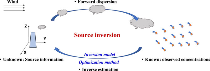
FIGURE 1. Concept diagram of source inversion.
A dispersion model with high efficiency and relatively high accuracy is generally required to conduct source inversion in small-scale regions in practice. From the viewpoint of practical applications (source term estimations and prediction concentrations) (MEPPRC, 2004; Senocak et al., 2008; Lushi and Stockie, 2011; Stockie, 2011; Ma et al., 2017; Ma et al., 2018), the Gaussian plume model was adopted in this study. According to the dispersion theory of the Gaussian model (Pasquill and Smith, 1983), the simulation concentration at any point in the downwind direction can be expressed as follows:
where C(x,y,z) is the pollutant concentration (g/m3) at the monitoring site (x,y,z) (m); Q0, y0, and z0 represent the pollutant emission rate parameter (g/s), horizontal crosswind location parameter (m), and the release height parameter (m);
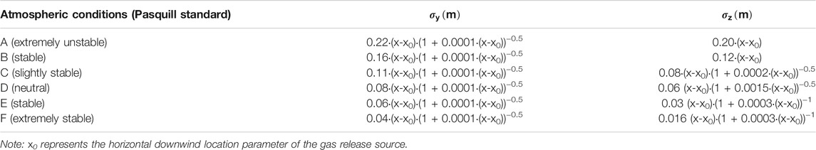
TABLE 1. Dispersion parameter schemes established by BRRIGS.
The widely used form of the sum of deviation squares (Zheng and Chen, 2010; Ma et al., 2018; Dong et al., 2020) was also used to construct the inversion models in this study, which is expressed as follows:
In Eq 2,
As described in the introduction section, different pollutant release types may correspond to different prior source location information available. According to the difference in location prior information, the source emission estimation of hazardous pollutants can be divided into two main cases: the known release source location (i.e., only source strength is unknown) and the unknown release source location (i.e., source strength and certain location parameters are unknown). In the case of an unknown release source location, it can be further divided into 1) only the release height is unknown (e.g., emissions from fires or certain industrial smokestacks), 2) only the horizontal location is unknown (e.g., emissions from near-ground source leakages), and 3) horizontal location and height are both unknown (e.g., emissions from near-ground or elevated source leakages). Thus, four source emission estimation scenarios were determined based on the aforementioned analysis, and four corresponding source emission inversion models were built by combining Eqs. 1, 2. The expressions under four source estimation scenarios are as follows:
Scenario 1 Only estimating source strength (single parameter estimation).
where
Scenario 2 Estimating both source strength and release height (double parameter estimation).
where
Scenario 3 Estimating both source strength and horizontal location (triple parameter estimation).
where
Scenario 4 Estimating source strength, horizontal location, and release height (quadruple parameter estimation).
where
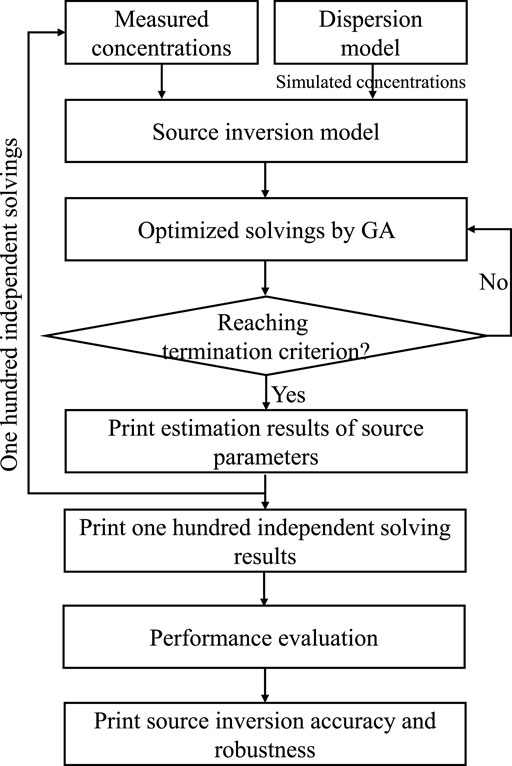
FIGURE 2. Flowchart of performance evaluation of source inversion.
Prairie Grass field experiments were conducted over a broad flat grassland in O’Neill, Nebraska, in 1956 (Barad, 1958). The overall roughness of the experimental site was approximately 6 cm. In total, 68 release experiments of SO2 were performed, and each experiment lasted for 10 min (Table 2). SO2 gas was continuously released as a point source at 0.46 or 1.5 m (the last six trials, i.e., numbers R63 to R68). The downwind sample collection adopted a semicircular arrangement of points and the base line of the horizontal sampling network was oriented along a true east–west line to take advantage of the prevailing southerly winds. Five arcs at distances of 50, 100, 200, 400, and 800 m from the release source were set as sampling arcs, and approximately 600 sensors were scattered along the sampling arcs to monitor downwind concentrations with a sampling height of 1.5 m. The coverage area of each sampling layer was 180°; the first four layers of sampling points were arranged at intervals of 1°, and the fifth layer was arranged at intervals of 2°. Wind speeds and wind direction at the height of 2 m above the ground were measured during the experiments by the cup anemometers and the means of airfoil-type vanes, respectively. Cervone and Franzese (2011) divided the dataset into six subset data of different atmospheric conditions based on the Pasquill atmospheric stability classification standard. The number of field experiments under Pasquill atmospheric stability classes A (extremely unstable), B (unstable), C (slightly unstable), D (neutral), E (stable), and F (extremely stable) were 5, 5, 10, 31, 5, and 12, respectively. To reflect the effects of atmospheric conditions in the real world, all valid detection concentrations above the sensor detection limit were used for each experiment.
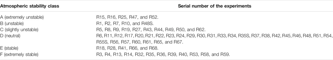
TABLE 2. Information of field experiments under different atmospheric conditions.
The absolute value of the relative deviation (ARD) of the source strength and the absolute value of deviation (AD) of the source location parameters were introduced to characterize the accuracy of the source inversion.
where E represents the inversion value, R represents the real value, Q is the source strength, J represents the serial number of the test experiment, and L represents the source location parameter (x0, y0, and z0).
The coefficient of variation (CV) was used to evaluate the robustness of the source inversion. The formula is as follows:
where
In this study, ARDs of the inversion results for 100 independent calculations for each field experiment were calculated first, then mean of 100 ARDs was taken as the result of each field experiment, and mean ARD of all field experiments for each atmospheric stability class was taken as the final result of each atmospheric stability class. The CV of each field experiment was calculated first based on the inversion results of 100 independent calculations, and the mean CV of all field experiments for each atmospheric stability class was taken as the final result of each atmospheric stability class.
Figure 3 shows the change progress of the best fitness value with evolutionary generations for GA optimization under different inversion scenarios. From the figure, as evolution progressed, the fitness value gradually declined. The process for searching source parameters under each inversion scenario stopped when the fitness value was less than the threshold value (i.e., 10–6). This indicates that the genetic algorithm can be successfully converged and efficiently applied to source parameter inversion.
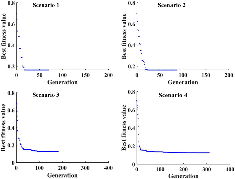
FIGURE 3. Change progress of best fitness value with evolutionary generations for GA optimization under different inversion scenarios: Scenario 1: only estimating source strength (Q0); (b) Scenario 2: estimating source strength (Q0) and release height (z0); Scenario 3: estimating both source strength (Q0) and horizontal location (x0, y0); Scenario 4: estimating source strength (Q0), horizontal location (x0, y0), and release height (z0).
Figure 4 shows the estimation accuracy and robustness of the source strength estimation under different inversion scenarios. Figures 4A,B show results for the single parameter and double parameter inversion. The atmospheric conditions had a similar effect on source strength inversion between the two inversion scenarios. Specifically, regarding the inversion accuracy, the comparable interquartile ranges, numerical distribution intervals of deviation data, mean values, and median values for these two scenarios under nearly all stability classes (except the stability class F) revealed that the impact of the pollutant release height parameter on the inversion accuracy of source strength was limited. The numerical distribution intervals of the deviations in the box under atmospheric stability classes A (extremely unstable condition) and F (extremely stable condition) were obviously higher than those under the other stability classes. These findings indicated that most experiments under stability classes A and F had large estimation deviations in source inversion. Notably, for the stability class A, the minimum and mean values of ARD under single (71.1 and 130.1%) and double (72.5 and 129.6%) parameter inversion were obviously larger than those of other stability classes. These aforementioned findings demonstrated that the inversion accuracy of source strength under extreme atmospheric conditions performed worse than the other conditions, wherein the inversion accuracy was the worst under extremely unstable atmospheric conditions. The worst inversion accuracy under extremely unstable atmospheric conditions might be the main reason for the significant decline in the simulation performance of the forward model for stability class A (Mao et al., 2020a). However, for the obviously large estimation deviations under extremely stable conditions, the reasons might have been mainly caused by the combined action of the poor simulation performance of the forward model (Mao et al., 2020a) and the fewer number of sensors with effective ground measurements owing to a smaller dispersion footprint (Cervone and Franzese, 2011; Cantelli et al., 2015). The aforementioned analysis indicated that the dominant factors that obviously reduced the inversion accuracy in two extreme atmospheric conditions were completely different. Additionally, there were obviously larger interquartile ranges of deviations under the atmospheric stability classes A (68.7 and 68.6% for single and double parameter inversion, respectively) and F (48.8 and 52.0% for single and double parameter inversion, respectively). This indicated that data in the box fluctuated greatly, representing a large difference in the inversion accuracy of different experiments under both stability classes. The reasons for large individual differences among these experiments in the inversion accuracy may also be attributed to the aforementioned factors. Conversely, the estimation accuracy of source inversion performed well under the stability classes B, C, D, and E because of small interquartile ranges and low numerical distribution intervals of inversion deviations, where the number of tested experiments with ARD less than 50.0% accounted for more than 75% in each stability class.
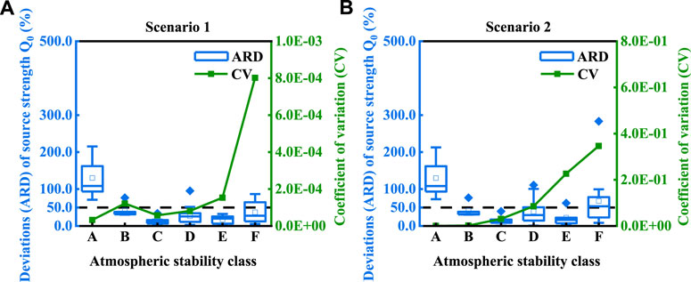
FIGURE 4. Boxplots of the inversion accuracy index (ARD) and line charts of the inversion robustness index (CV) for source strength (Q0) estimation under different application scenarios: (A) Scenario 1: only estimating source strength (Q0), and (B) Scenario 2: estimating source strength (Q0) and release height (z0).
For robustness, CVs in all stability classes for single parameter inversion (<0.001) and double parameter inversion (<0.4) were both at a relatively low level. This suggested that the atmospheric conditions had only a limited impact on inversion robustness. There were slightly higher values of CVs under the atmospheric stability class F than under other stability classes. It indicated that the inversion robustness performed relatively worse under extremely stable atmospheric conditions. However, comparing the results of Figures 4A,B, the CV of the double parameter inversion was obviously higher than that of the single parameter inversion by more than an order of magnitude in each stability class. This phenomenon indicated that the inversion robustness of the source strength largely declined as the unknown parameter was added to the source height. Figures 5A,B show the results under inversion scenarios of triple and quadruple parameters. These figures reveal that the variation characteristics of the parameter inversion performance under atmospheric conditions under these two scenarios were also similar. Regarding accuracy, similar to single and double parameter scenarios, the comparable interquartile ranges, numerical distribution intervals of deviation data, mean values, and median values for these two scenarios under each stability class revealed that the vertical release height parameter had little influence on the inversion accuracy of source strength. The numerical distribution intervals of the deviation data in the box under unstable atmospheric conditions (stability classes A, B, and C) were obviously higher than those in the box under neutral (stability class D) and stable conditions (stability classes E and F), with most ARDs larger than 50.0%. However, the interquartile ranges (202.8 and 203.2% for triple and quadruple parameter inversion, respectively), and minimum values of ARD (225.2 and 225.0% triple and quadruple parameter inversion, respectively) under the stability class B were much larger than those of the other two unstable stability classes. This finding suggests that the inversion accuracy for unstable atmospheric conditions was obviously worse than that for extremely unstable and slightly unstable dispersion conditions. However, what seems to be contradictory is that the inversion accuracy under unstable conditions (stability class B) was obviously worse than that under extremely unstable conditions (stability class A). This phenomenon was also found by Cui et al. (2019) where the source inversion performance was evaluated under different stability classes based on another optimization algorithm (PSO-NM). Cervone and Franzese et al. (2011) summarized the calculated error between the simulated and observed concentrations under all the 68 Prairie Grass field experiments and found that four out of the five experiments had a remarkably larger margin of errors between the simulated and observed concentrations under the stability class B. Meanwhile, Cantelli et al. (2015) investigated the relationship between the averaged wind direction standard deviation and distance errors of source location inversion and found that the worst inversion performance of source location was associated with high values of the measured averaged wind direction standard deviation. It is worthy to note that this phenomenon had no relation with single and double parameter scenarios. This might be related to the fact that the horizontal location parameter increased the complexity of solving nonlinear problems. Thus, in summary, the large uncertainty of inversion results under unstable conditions may be attributed to two factors including the large simulation error of the forward model due to insufficient description for the turbulent characteristics of the dynamic wind field by the model itself and the nonlinear degree variation with the addition of unknown horizontal location parameters. On the whole, from unstable to slightly stable atmospheric conditions (i.e., stability classes A–E), the inversion accuracy generally tended to increase because the interquartile ranges, mean values, and median values all showed a decreasing tendency. This finding indicates that the inversion accuracy gradually improved with the stabilization of atmospheric conditions. However, large interquartile ranges and the mean value of ARD occurred when the atmospheric dispersion condition developed to an extremely stable state (i.e., the stability class F). This finding indicated that the extremely stable condition increased the uncertainty of the inversion deviations of the source strength. Our results of atmospheric condition influence based on the classical GA method are basically consistent with those based on improved algorithms (PSO-NM, Cui et al., 2019; non-Darwinian evolutionary algorithm, Cervone and Farnese, 2011) when applied to the same Prairie Grass experiments and under the same inversion scenarios. However, different conclusions stating that the inversion accuracy under the A and B classes performed relatively well were drawn by Catelli et al. (2015). This is mainly caused by the difference in evaluation methods of inversion results. In the study by Cantelli et al., the inversion performance was evaluated by comparing the number of experiments in which the inversion deviation exceeded a certain value under different stability degrees, whereas the inversion performance was evaluated by calculating the mean value of the inversion deviation of all experiments in the present and previous studies (i.e., Cui et al., 2019; Cervone and Franzese, 2011).
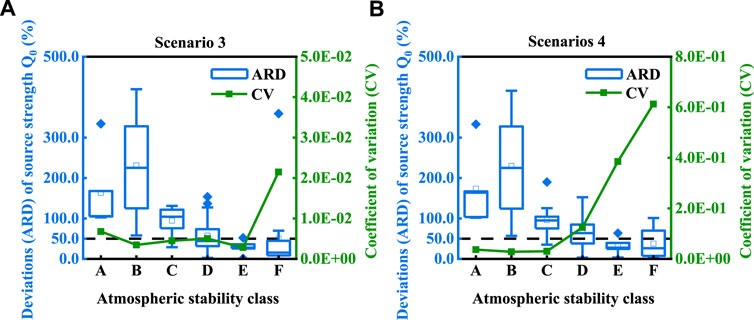
FIGURE 5. Boxplots of the inversion accuracy index (ARD) and line charts of the inversion robustness index (CV) for source strength (Q0) estimation under different application scenarios: (A) Scenario 3: estimating both source strength (Q0) and horizontal location (x0, y0), and (B) Scenario 4: estimating source strength (Q0), horizontal location (x0, y0), and release height (z0).
Comparing the different scenarios, the mean ARDs of 68 experiments were 34.4, 46.0, 80.1, and 83.6% for single parameter, double parameters, triple parameters, and quadruple parameters, respectively. This indicated that the estimation accuracy of source strength gradually worsened with an increase in the number of unknown source parameters. Additionally, by comparing the scenarios of single and double parameters and the scenarios of triple and quadruple parameters, it was obviously found that source release height had a minimal effect on the estimation accuracy; whereas, by comparing the scenarios of single and triple parameters and the scenarios of double and quadruple parameters, it was obviously found that source horizontal location largely affected the estimation accuracy. This indicated that the unknown source horizontal location parameters were important factors influencing the accuracy of source strength inversion and source release height only had limited influence.
For robustness, there were obviously higher values of CVs under the atmospheric stability class F (0.02 and 0.61 for the triple and quadruple parameter inversions, respectively) than those of other stability classes. This phenomenon is similar to the single and double parameter inversions. The robustness performed worse in the case of quadruple parameter inversion than in the case of triple parameter inversion under each stability class because the CVs were obviously larger (0.037, 0.028, 0,03, 0.124, 0.385, and 0.613 for the stability classes A, B, C, D, E, and F, respectively) when four parameters were both estimated. Notably, a remarkable picture occurred when we compared the robustness of the source strength estimation under all scenarios: CVs had more than one order of magnitude and were smaller under triple parameter inversion than under double and quadruple parameter inversion in all atmospheric conditions except for the stability classes A and B; and although the CVs of quadruple parameter inversion were generally higher than those of double parameter inversion, they were of the same order of magnitude as those of double parameter inversion. These findings indicated that the inversion robustness did not necessarily deteriorate as expected with an increase in the number of unknown parameters, whereas, it was obviously affected by the type of the unknown source location parameter. In other words, the inversion robustness was more susceptible to source release height parameter in the source strength estimation and relatively insensitive to horizontal positional parameters.
Accurately locating pollutant sources is also important in some scenarios, especially in the case of toxic gas release caused by an accidental leak or terrorist acts (Ma et al., 2018). Figure 6 shows the estimation deviations and CV for source location parameters (i.e., x0, y0, z0) estimation under different inversion scenarios. Figure 6A shows the results of the inversion performance indicators of horizontal location x0 under triple and quadruple parameter inversion. Regarding accuracy, the variation characteristics of inversion deviations under the effects of atmospheric conditions were similar for these two inversion scenarios. The magnitude of the deviation values was very close under each stability class (A, B, C, D, E, and F) for triple parameter inversion (14.6, 74.2, 21.5, 27.4, 20.4, and 94.7 m) and quadruple parameter inversion (14.7, 73.9, 19.0, 27.6, 23.3 and 99.4 m). Obviously, the estimation accuracy of location x0 changed little with the addition of release height parameters. This indicated that the inversion accuracy of location x0 was insensitive to the source release height. The higher numerical distribution intervals of the deviation data, larger mean values, and median values for the stability classes B and F than for other stability classes suggested that the inversion accuracy was obviously worse in unstable and extremely stable atmospheric conditions. The relatively larger interquartile ranges for the stability classes B and F indicated that there were larger fluctuations of inversion deviation for different experiments. These findings for location x0 were similar to source strength Q0. The inversion accuracy performed relatively well with low numerical distribution intervals (most ADs <50.0 m) for stability classes A, C, D, and E. For robustness, all CVs were at a low level, with values less than 0.1. This finding indicated that the inversion robustness performed well in estimating the location x0. However, there were large differences in the robustness. The CV of each stability class (A, B, C, D, E, and F) was obviously higher for quadruple parameter inversion (0.102, 0.021, 0.045, 0.093, 0.061, and 0.137) than that of triple parameter inversion (0.060, 0.005, 0.020, 0.080. 0.014, and 0.020). This finding indicated that the inversion robustness of location parameter x0 was obviously affected by the unknown source height parameter. Figure 6B shows the comparison results of the inversion performance indicators of the horizontal location y0. Overall, the variation characteristics of the inversion accuracy with atmospheric conditions were consistent for the two inversion scenarios. Interquartile ranges and minimum values of inversion deviations were comparable for the triple and quadruple parameter inversion scenarios. Compared with parameter x0, inversion deviations were obviously reduced, with deviations less than 10.0 m in most experiments. For robustness, the largest CVs for triple parameter inversion and quadruple parameter inversion were obtained in stability classes C (0.11) and B (0.40), respectively. Overall, CVs of the triple parameter inversion were slightly lower than those of the quadruple parameter inversion in most atmospheric conditions. Figure 6C shows the comparison results of the inversion performance indicators of the source release height z0. There were only slight differences between the double parameter inversion and quadruple parameter inversion scenarios in accuracy under each atmospheric stability class, and the deviations under the two inversion scenarios were very low (< 4.0 m). Regarding robustness, similar decline characteristics of the robustness with the atmospheric condition variation occurred, and the highest CVs (0.69 and 0.59 for triple and quadruple parameter inversions, respectively) occurred under extreme conditions (stability class F).
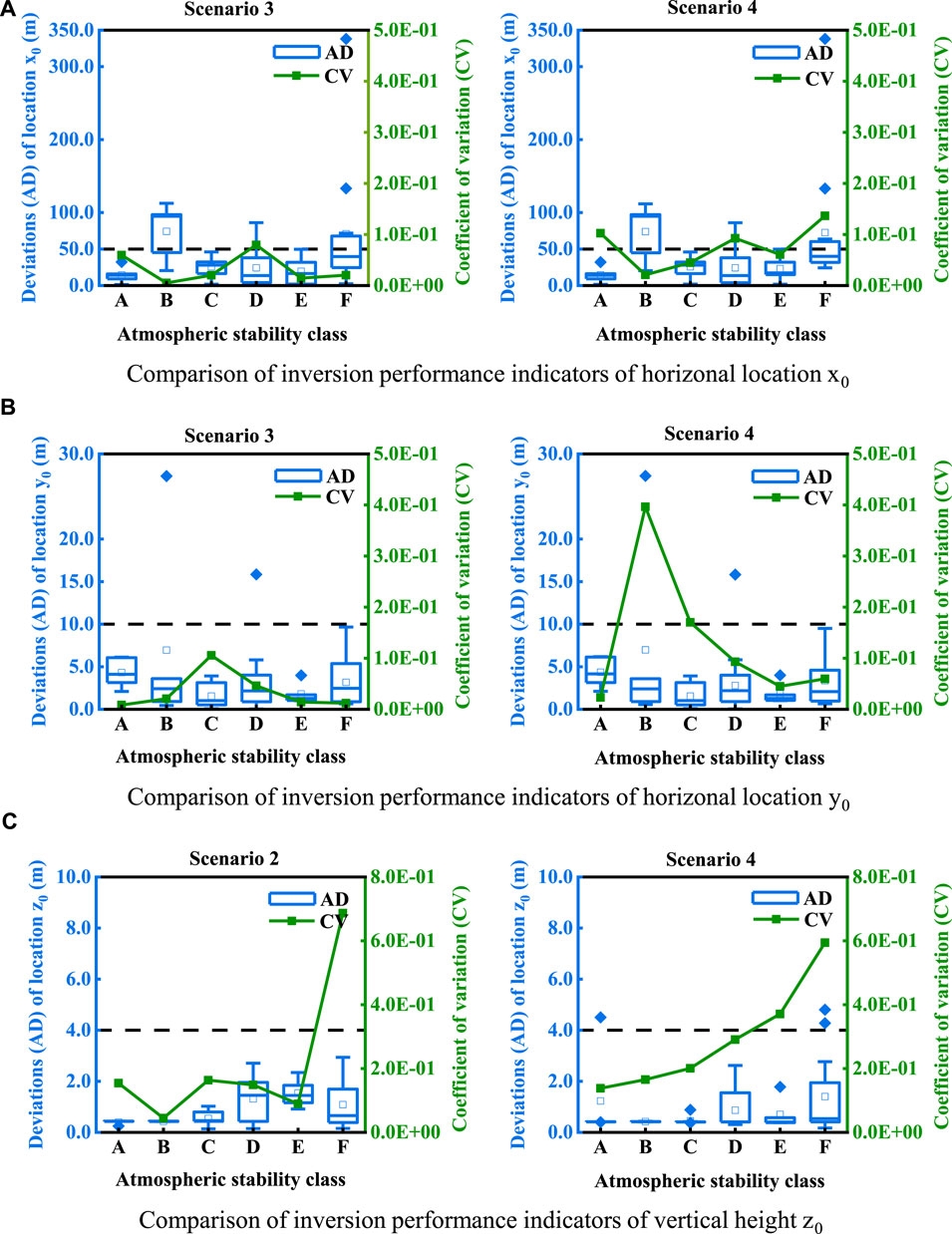
FIGURE 6. Boxplots of the inversion accuracy index (AD) and line charts of the inversion robustness index (CV) for source location (i.e., x0, y0, and z0) estimation. (A) Comparison of inversion performance indicators of the horizontal location parameter x0, (B) comparison of inversion performance indicators of the horizontal location parameter y0, and (C) comparison of inversion performance indicators of the vertical height parameter z0.
The practical application and popularization of optimized source inversion technology must overcome substantial challenges because complex, real air pollution accident scenes generally correspond to different source inversion scenarios. This study investigated the performance variation law of optimization source inversion in small-scale regions (<1 km) under multiple scenarios involving different atmospheric conditions (stability class A–F) and unknown source parameters (source strength and location) and further explored the influencing mechanism of different location parameters on the estimation performance of source strength. The results showed that atmospheric conditions had different impacts on the source strength inversion under different parameter inversion scenarios. Extreme atmospheric conditions (stability classes A and F) can obviously reduce the estimation accuracy of source strength for single and double parameter inversion scenarios. However, the dominant factors that reduced the inversion accuracy in two extreme atmospheric conditions were completely different. Thereinto, the poor inversion accuracy under stability class A may mainly be attributed to poor model simulations. However, the poor performance under the stability class F was caused by the combined actions of the poor model simulations and the fewer available sensors. However, for triple and quadruple parameter scenarios, the estimation accuracy of the source strength was worse under unstable atmospheric conditions (stability classes A, B, and C) than that under other atmospheric conditions. Thereinto, a contradiction occurred stating that the inversion accuracy under unstable conditions (stability class B) was worse than that under extremely unstable conditions. This large uncertainty of inversion results may be attributed to the combined effects of the increase in the complexity of nonlinearity problem with the addition of horizontal location parameters and poor model simulation performance caused by the insufficient description for the dynamic wind field. Relationship analysis between estimation performance of source strength and source location revealed that source strength inversion performance was affected by location parameters; robustness was markedly reduced when source height was unknown, whereas accuracy was obviously reduced when source horizontal location parameters were unknown.
These new findings in this article can fill the knowledge gap in the characteristic laws of optimized source inversion technology under complex application scenarios and the interaction relationship between different unknown source parameters. The results of the influence mechanism of source location prior information on source strength have important guiding significance to further improving the inversion accuracy of source strength in practical environmental management. Additionally, this study quantified the uncertainty of the inversion results under multiple specific scenarios based on sufficient experimental data. This can provide a reference for pollutant emission estimation in small-scale flat terrains (e.g., small-scale industrial parks distributed in flat rural or suburban areas) in real applications. However, the limitations of this study should be investigated in further research. For example, the number of experiments used in some atmospheric stability classes (i.e., stability A, B, and E) was small. This may have caused uncertainties in the results. For a limited number of searching problems (less than four variables) in this study, the GA may not be the optimal method in searching solutions when the factors such as solving efficiency, absolute accuracy, and so on were considered. Thus, a more appropriate optimization method should be selected according to the requirements in actual research studies or real-world applications. Furthermore, the conclusions may provide a limited application reference in practice for more complex scenarios (e.g., urban and long-range scale) because the basic dataset used is from a flat grassland terrain on a small scale, and the dispersion model is a relatively simple Gaussian model where the pollution dispersion process under complex terrains cannot be well described. Additionally, this study did not focus on the secondary chemical transformation of pollutants; therefore, the study results may not be successfully applied to secondary pollutants.
This study investigated the estimation performance of source optimization inversion under multiple application scenarios involving different atmospheric dispersion conditions and inversion parameters. Four source inversion models were constructed based on typical application scenarios of source estimation. The genetic algorithm was selected as the optimization inversion method, and the Prairie Grass dataset, including 68 experiments, was selected as the basic data to evaluate the estimation performance. The results showed that the atmospheric conditions obviously affected the source strength inversion performance. The atmospheric conditions had similar effect characteristics on the source strength inversion for the single and double parameter inversion scenarios. The source inversion performed poorly with regard to the estimation accuracy of source strength under extremely unstable (stability class A) and stable (stability class F) atmospheric conditions. However, the robustness of source strength estimation was obviously poor under only extremely unstable atmospheric conditions (stability class F). For the triple and quadruple parameter inversion scenarios, similar performances were also shown; that is, the inversion accuracy of the source strength was worse under unstable atmospheric conditions (stability classes A, B, and C) than under other atmospheric conditions. As for robustness, similar to the single and double parameter inversions, there were obviously high values of the CV under the atmospheric stability class F. Comparative results of the four inversion scenarios indicated that the estimation accuracy of source strength declined with an increase in the number of unknown source parameters. The estimation accuracy of the source strength obviously declined when the horizontal location parameters were unknown, and the estimation robustness of the source strength greatly declined when the source height parameter was unknown. The results of location parameter inversion showed that, for parameter x0, the variation characteristics of inversion accuracy under different atmospheric conditions were essentially consistent for the two scenarios. The robustness of source inversion is vulnerable to the unknown source height parameter, whereas the inversion accuracy is not sensitive to the unknown source height. There were obviously smaller estimation deviation distribution ranges for the parameters y0 and z0 than for the parameter x0. Furthermore, there was a little difference in the accuracy of the two parameters y0 and z0 under different inversion scenarios. Regarding robustness, related to the parameter y0, the performance was relatively worse owing to the addition of an unknown source height parameter. Regarding the parameter z0, similar decline characteristics of robustness occurred with variations in atmospheric conditions; the highest CVs occurred under extreme conditions (stability class F). This study can deepen the understanding of the impacts of external environmental factors on source inversion and provide a reference for pollutant emission estimation and location tracking of air pollution events in small-scale flat terrains in practice.
Publicly available datasets were analyzed in this study. These data can be found here: Barad, M.L. (1958). PROJECT PRAIRIE GRASS, A FIELD PROGRAM IN DIFFUSION. Air Force Cambridge Research Center, Bedford, United States, pp. 300.
LJ contributed to the conception and design of the study. SM organized the database and wrote the first draft of the manuscript. TC and SC edited the manuscript. FH performed the statistical analysis. All authors contributed to manuscript revision, read, and approved the submitted version.
This research was financially supported by the National Key R&D Program of China (No. 2017YFC0209905) and Beijing Nova Program (Z201100006820098) of the Beijing Municipal Science and Technology Commission.
The authors declare that the research was conducted in the absence of any commercial or financial relationships that could be construed as a potential conflict of interest.
All claims expressed in this article are solely those of the authors and do not necessarily represent those of their affiliated organizations, or those of the publisher, the editors, and the reviewers. Any product that may be evaluated in this article, or claim that may be made by its manufacturer, is not guaranteed or endorsed by the publisher.
The authors are grateful to the reviewers for their insightful comments. In addition, we greatly appreciate the Beijing Municipal Education Commission for supporting this work.
Amoatey, P., Omidvarborna, H., Baawain, M. S., and Al-Mamun, A. (2019). Emissions and Exposure Assessments of SOX, NOX, PM10/2.5 and Trace Metals from Oil Industries: A Review Study (2000-2018). Process Saf. Environ. Prot. 123, 215–228. doi:10.1016/j.psep.2019.01.014
Barad, M. L. (1958). PROJECT PRAIRIE GRASS, A FIELD PROGRAM IN DIFFUSION. Bedford, USA: Air Force Cambridge Research Center, 300.
Bildirici, M. E. (2017). The Effects of Militarization on Biofuel Consumption and CO 2 Emission. J. Clean. Prod. 152, 420–428. doi:10.1016/j.jclepro.2017.03.103
Briggs, G. A. (1973). Diffusion Estimation for Small Emissions. Oak Ridge, TN: Atmospheric Turbulence and Diffusion Laboratory, NOAA. ATDL Contribution File NO.79.
Cantelli, A., D'orta, F., Cattini, A., Sebastianelli, F., and Cedola, L. (2015). Application of Genetic Algorithm for the Simultaneous Identification of Atmospheric Pollution Sources. Atmos. Environ. 115, 36–46. doi:10.1016/j.atmosenv.2015.05.030
Cervone, G., and Franzese, P. (2011). Non-Darwinian Evolution for the Source Detection of Atmospheric Releases. Atmos. Environ. 45, 4497–4506. doi:10.1016/j.atmosenv.2011.04.054
Chen, H., and Carter, K. E. (2020). Hazardous Substances as the Dominant Non-methane Volatile Organic Compounds with Potential Emissions from Liquid Storage Tanks during Well Fracturing: A Modeling Approach. J. Environ. Manage. 268, 110715. doi:10.1016/j.jenvman.2020.110715
Clappier, A., and Thunis, P. (2020). A Probabilistic Approach to Screen and Improve Emission Inventories. Atmos. Environ. 242, 117831. doi:10.1016/j.atmosenv.2020.117831
Cui, J., Lang, J., Chen, T., Cheng, S., Shen, Z., and Mao, S. (2019). Investigating the Impacts of Atmospheric Diffusion Conditions on Source Parameter Identification Based on an Optimized Inverse Modelling Method. Atmos. Environ. 205, 19–29. doi:10.1016/j.atmosenv.2019.02.035
Dong, J., Du, W., Wang, B., and Xu, Q. (2020). Investigating Impacts of Cost Functions to Atmospheric Dispersion Modeling and Source Term Estimation in Turbulent Condition. CIESC J. 71 (3), 1163–1173. (Chinese). doi:10.11949/0438-1157.20191550
Du, L., Wang, H., and Xu, H. (2020). Analysis of Spatial-Temporal Association and Factors Influencing Environmental Pollution Incidents in China. Environ. Impact Assess. Rev. 82, 106384. doi:10.1016/j.eiar.2020.106384
Gao, Z., Desjardins, R. L., and Flesch, T. K. (2009). Comparison of a Simplified Micrometeorological Mass Difference Technique and an Inverse Dispersion Technique for Estimating Methane Emissions from Small Area Sources. Agric. For. Meteorology 149, 891–898. doi:10.1016/j.agrformet.2008.11.005
Hamblin, S. (2013). On the Practical Usage of Genetic Algorithms in Ecology and Evolution. Methods Ecol. Evol. 4, 184–194. doi:10.1111/2041-210X.12000
Haupt, S. E. (2005). A Demonstration of Coupled Receptor/dispersion Modeling with a Genetic Algorithm. Atmos. Environ. 39, 7181–7189. doi:10.1016/j.atmosenv.2005.08.027
Haupt, S. E., Young, G. S., and Allen, C. T. (2006). Validation of a Receptor-Dispersion Model Coupled with a Genetic Algorithm Using Synthetic Data. J. Appl. Meteorology Climatology 45, 476–490. doi:10.1175/JAM2359.1
Jeričević, A., Gašparac, G., Mikulec, M. M., Kumar, P., and Prtenjak, M. T. (2019). Identification of Diverse Air Pollution Sources in a Complex Urban Area of Croatia. J. Environ. Manage. 243, 67–77. doi:10.1016/j.jenvman.2019.04.024
Koutsomarkos, V., Rush, D., Jomaas, G., and Law, A. (2021). Tactics, Objectives, and Choices: Building a Fire Risk index. Fire Saf. J. 119, 103241. doi:10.1016/j.firesaf.2020.103241
Lei, J., Miao, X., Liu, Z., Liu, N., and Zhang, L. (2021). Lifted Flame in Fire Whirl: An Experimental Investigation. Proc. Combustion Inst. 38, 4595–4603. doi:10.1016/j.proci.2020.07.087
Lin, Y.-C., Lai, C.-Y., and Chu, C.-P. (2021). Air Pollution Diffusion Simulation and Seasonal Spatial Risk Analysis for Industrial Areas. Environ. Res. 194, 110693. doi:10.1016/j.envres.2020.110693
Liu, Y., Han, F., Liu, W., Cui, X., Luan, X., and Cui, Z. (2020). Process-based Volatile Organic Compound Emission Inventory Establishment Method for the Petroleum Refining Industry. J. Clean. Prod. 263, 121609. doi:10.1016/j.jclepro.2020.121609
Long, K. J., Haupt, S. E., and Young, G. S. (2010). Assessing Sensitivity of Source Term Estimation. Atmos. Environ. 44, 1558–1567. doi:10.1016/j.atmosenv.2010.01.003
Lushi, E., and Stockie, J. M. (2010). An Inverse Gaussian Plume Approach for Estimating Atmospheric Pollutant Emissions from Multiple point Sources. Atmos. Environ. 44, 1097–1107. doi:10.1016/j.atmosenv.2009.11.039
Ma, D., Tan, W., Zhang, Z., and Hu, J. (2017). Parameter Identification for Continuous point Emission Source Based on Tikhonov Regularization Method Coupled with Particle Swarm Optimization Algorithm. J. Hazard. Mater. 325, 239–250. doi:10.1016/j.jhazmat.2016.11.071
Ma, D., Tan, W., Wang, Q., Zhang, Z., Gao, J., Wang, X., et al. (2018). Location of Contaminant Emission Source in Atmosphere Based on Optimal Correlated Matching of Concentration Distribution. Process Saf. Environ. Prot. 117, 498–510. doi:10.1016/j.psep.2018.05.028
Mao, S., Lang, J., Chen, T., Cheng, S., Cui, J., Shen, Z., et al. (2020a). Comparison of the Impacts of Empirical Power-Law Dispersion Schemes on Simulations of Pollutant Dispersion during Different Atmospheric Conditions. Atmos. Environ. 224, 117317. doi:10.1016/j.atmosenv.2020.117317
Mao, S., Lang, J., Chen, T., Cheng, S., Wang, C., Zhang, J., et al. (2020b). Impacts of Typical Atmospheric Dispersion Schemes on Source Inversion. Atmos. Environ. 232, 117572. doi:10.1016/j.atmosenv.2020.117572
Mao, S., Lang, J., Chen, T., and Cheng, S. (2021). Improving Source Inversion Performance of Airborne Pollutant Emissions by Modifying Atmospheric Dispersion Scheme through Sensitivity Analysis Combined with Optimization Model. Environ. Pollut. 284, 117186. doi:10.1016/j.envpol.2021.117186
Mepprc, (2004). Technical Guidelines for Environmental Risk Assessment on Projects (HJ/T 169-2004). (Chinese) Available from: http://kjs.mep.gov.cn/hjbhbz/bzwb/other/pjjsdz/200412/W020110127329297430823.pdf.
Senocak, I., Hengartner, N. W., Short, M. B., and Daniel, W. B. (2008). Stochastic Event Reconstruction of Atmospheric Contaminant Dispersion Using Bayesian Inference. Atmos. Environ. 42, 7718–7727. doi:10.1016/j.atmosenv.2008.05.024
Singh, S. K., and Rani, R. (2014). A Least-Squares Inversion Technique for Identification of a point Release: Application to Fusion Field Trials 2007. Atmos. Environ. 92, 104–117. doi:10.1016/j.atmosenv.2014.04.012
Singh, S. K., and Rani, R. (2015). Assimilation of Concentration Measurements for Retrieving Multiple point Releases in Atmosphere: A Least-Squares Approach to Inverse Modelling. Atmos. Environ. 119, 402–414. doi:10.1016/j.atmosenv.2015.08.063
Stockie, J. M. (2011). The Mathematics of Atmospheric Dispersion Modeling. SIAM Rev. 53, 349–372. doi:10.1137/10080991x
Stohl, A., Seibert, P., Wotawa, G., Arnold, D., Burkhart, J. F., Eckhardt, S., et al. (2012). Xenon-133 and Caesium-137 Releases into the Atmosphere from the Fukushima Dai-Ichi Nuclear Power Plant: Determination of the Source Term, Atmospheric Dispersion, and Deposition. Atmos. Chem. Phys. 12 (5), 2313–2343. doi:10.5194/acp-12-2313-2012
Thomson, L. C., Hirst, B., Gibson, G., Gillespie, S., Jonathan, P., Skeldon, K. D., et al. (2007). An Improved Algorithm for Locating a Gas Source Using Inverse Methods. Atmos. Environ. 41, 1128–1134. doi:10.1016/j.atmosenv.2006.10.003
Wang, Y., Huang, H., Huang, L., and Zhang, X. (2018). Source Term Estimation of Hazardous Material Releases Using Hybrid Genetic Algorithm with Composite Cost Functions. Eng. Appl. Artif. Intelligence 75, 102–113. doi:10.1016/j.engappai.2018.08.005
Wang, X., Lei, Y., Yan, L., Liu, T., Zhang, Q., and He, K. (2019). A Unit-Based Emission Inventory of SO2, NOx and PM for the Chinese Iron and Steel Industry from 2010 to 2015. Sci. Total Environ. 676, 18–30. doi:10.1016/j.scitotenv.2019.04.241
Wang, Y., Chen, B., Zhu, Z., Wang, R., Chen, F., Zhao, Y., et al. (2020). A Hybrid Strategy on Combining Different Optimization Algorithms for Hazardous Gas Source Term Estimation in Field Cases. Process Saf. Environ. Prot. 138, 27–38. doi:10.1016/j.psep.2020.02.029
Wang, Y., Zhang, R., Worden, S., Cao, H., and Li, C. (2021). Public Participation in Environmental Governance Initiatives of Chemical Industrial parks. J. Clean. Prod. 305, 127092. doi:10.1016/j.jclepro.2021.127092
Wei, W., Cheng, S., Li, G., Wang, G., and Wang, H. (2014). Characteristics of Ozone and Ozone Precursors (VOCs and NOx) Around a Petroleum Refinery in Beijing, China. J. Environ. Sci. 26, 332–342. doi:10.1016/S1001-0742(13)60412-X
Zheng, X., and Chen, Z. (2010). Back-calculation of the Strength and Location of Hazardous Materials Releases Using the Pattern Search Method. J. Hazard. Mater. 183, 474–481. doi:10.1016/j.jhazmat.2010.07.048
Keywords: air pollution, source parameter estimation, inversion modeling, atmospheric dispersion conditions, multiple pollutant emission scenarios, small-scale regions
Citation: Mao S, Lang J, Chen T, Cheng S and Hu F (2022) Comparative Study of Source Inversion Under Multiple Atmospheric Pollutant Emission Scenarios. Front. Environ. Sci. 10:857701. doi: 10.3389/fenvs.2022.857701
Received: 19 January 2022; Accepted: 11 February 2022;
Published: 17 March 2022.
Edited by:
Hongmei Xu, Xi’an Jiaotong University, ChinaReviewed by:
Wei Sun, Sun Yat-Sen University, ChinaCopyright © 2022 Mao, Lang, Chen, Cheng and Hu. This is an open-access article distributed under the terms of the Creative Commons Attribution License (CC BY). The use, distribution or reproduction in other forums is permitted, provided the original author(s) and the copyright owner(s) are credited and that the original publication in this journal is cited, in accordance with accepted academic practice. No use, distribution or reproduction is permitted which does not comply with these terms.
*Correspondence: Jianlei Lang, amxsYW5nQGJqdXQuZWR1LmNu
Disclaimer: All claims expressed in this article are solely those of the authors and do not necessarily represent those of their affiliated organizations, or those of the publisher, the editors and the reviewers. Any product that may be evaluated in this article or claim that may be made by its manufacturer is not guaranteed or endorsed by the publisher.
Research integrity at Frontiers
Learn more about the work of our research integrity team to safeguard the quality of each article we publish.