Coupling the TEB and Surfatm Models for Heat Flux Modelling in Urban Area: Comparison With Flux Measurements in Strasbourg (France)

This study presents the coupling of TEB (Town Energy Balance) and Surfatm models developed for energy exchange estimates for urban impervious and vegetation surfaces, respectively. Once coupled, the TEB-Surfatm model allows the estimate of radiative, sensible (H), and latent heat (LE) fluxes in urban areas accounting for urban vegetation. The modelled fluxes were compared with measurements performed in an urban garden. The model was able to reproduce the energy fluxes, but its performance varied. The variability of the model accuracy depended on the measurement footprint in link with the heterogeneity of the site characteristics: while the measurement footprint fitted with the area characteristics considered by the TEB-Surfatm model, the modelled H and LE fluxes presented a good agreement with the measurements. In the other cases, some overestimation and underestimation occurred, in link with different fractions of impervious surfaces or green spaces. The validation of the TEB-Surfatm model for energy fluxes is a first step, the second will be to include the pollutant exchanges since Surfatm is able to quantify the atmosphere-biosphere fluxes for numerous pollutants. It will allow the TEB-Surfatm model to quantify the impact of urban greening on the assessment of air quality in urban areas.

1 Introduction

Urban spaces are areas of great attractiveness. Nowadays, 55% of the world population lives in urban areas and it is expected 68% by 2050 (United Nations, Department of Economic and Social Affairs, and Population Division, 2019). Urban places occupied between 1.86 and 2.00% in 1985 and currently reach 3% of the continental Earth’ surface excluding Antarctica and Greenland (Liu et al., 2014). However, the urbanization leads to numerous modifications of the environment and in particular of the microclimate i.e., the so-called urban heat island (UHI) phenomenon (Oke, 1982). It refers to the fact that urban areas are warmer than their surroundings. This phenomenon, by modifying local microclimate, can affect air pollution (e.g., Rosenfeld et al., 1998; Akbari et al., 2001; Sarrat et al., 2006), induce convective thunderstorms (e.g., Bornstein and Lin, 2000), and enhance energy consumption for building cooling requirements (e.g., Akbari et al., 2001; Li et al., 2014). Yet, the excess of heat alters the human comfort and extreme heat events can lead to mortality (Vandentorren et al., 2004; Duneier, 2006; Harlan and Ruddell, 2011).

The UHI is due to many factors in link with urbanization which modifies the surface radiative budget and energy balance (Nunez and Oke, 1977; Oke, 1982). The solar radiation is absorbed by surfaces due the low albedo materials of infrastructures compared to natural ecosystems and agrosystems (Bouyer et al., 2009; Santamouris et al., 2011) and is released by them at night due to higher thermal inertia of urban materials (Pratt and Ellyett, 1979; Johnson et al., 1991; Berwal et al., 2016). Yet, the three dimensional geometry of the cities traps radiations (diminishing the whole city albedo and emissivity). It also prevents the wind from circulating depending on the orientation of the street; which leads to heat stagnation into the canyon constituted by a street and the surrounding buildings (Nuruzzaman, 2015). Additionally, human activities generate anthropogenic heat releases throughout e.g., high road traffic or building heating/cooling systems (Pigeon et al., 2007). Last but not least the lack of vegetation, trees, shrubs, and meadows in these areas induces less energy dissipation through latent heat flux to the benefit of sensible heat flux responsible for city warming (Pearlmutter et al., 2009). The UHI intensity is defined as the temperature difference between the inner city and its surroundings. The UHI intensity is greater at night, in summer, and under anticyclonic conditions. It decreases with cloudy cover and high wind speed. The intensity of UHI depends overall on the size of the city and/or population, the greening proportion, and the urban morphology (Arnfield, 2003). The UHI intensity is therefore highly variable on the spatial and temporal scales and can range from 0.6 °C to up to 10 °C (Memon et al., 2009).

Many studies have explored techniques to counterbalance the UHI. On the one hand, these techniques concerned the development of the so-called “cool” materials characterized by both high emissivity and reflectivity (Rosenfeld et al., 1998; Synnefa et al., 2008; Santamouris, 2013; Alchapar et al., 2014; Radhi et al., 2014; Rossi et al., 2014). On the other hand, researchers focused their attention on mitigation strategies based on macro scale approach by exploring the role of urban form, urban fabric, and building arrangement and orientation (Stone and Norman, 2006; Emmanuel and Fernando, 2007; Shahmohamadi et al., 2010; Middel et al., 2014). Nevertheless, green surfaces such as parks, gardens, or green roofs and walls can also help to mitigate the UHI and currently receive strong attention from scientists and urban planners (e.g. Shashua-Bar and Hoffman, 2000; Akbari et al., 2001; Kumar and Kaushik, 2005; Alexandri and Jones, 2008; Feyisa et al., 2014). However the cooling effect provided by vegetation is difficult to quantify due to the complexity of the processes involved and the numerous parameters and variables controlling both UHI intensity and vegetation cooling potential. Cooling potential depends on the type of vegetation and local climatic conditions. For instance, Bowler et al. (2010) list impacts of different type of greening surfaces on cooling effect: grass parks tended to be warmer than parks with tree covers at diurnal time due to the shading effect of trees. Yet, Shashua-Bar and Hoffman (2000) reported that the cooling effect of trees is greater under warm conditions.

Evapotranspiration is considered as one of the most important factor of cooling effect (Taha, 1997; Shashua-Bar and Hoffman, 2000; Dimoudi and Nikolopoulou, 2003; Qiu et al., 2013). However, plant species exhibit significant differences in their evapotranspiration rates due to their different stomatal conductance and leaf area density (Gillner et al., 2015). Therefore, some differences in terms of vegetation cooling potential occur between e.g., individual vegetation and parks or dense vegetation area such as urban forests. Indeed, during daytime cooling effect is greater for dense vegetation but some heat storage at night can occur. Hence, a modelling approach is necessary to account for all these complex physical and biological processes controlled by urban characteristics and pedoclimatic conditions.

Many models have been developed to simulate the energy exchanges between the built-up areas and the atmosphere in order to quantify the impact of urbanization on microclimate, as well as the benefits from urban greening. Overall, they can be sorted in two categories: the high resolution models based on computational fluid dynamics (e.g., Solene microclimate, ENVImet, LASER/F) (Bruse and Fleer, 1998; Bouyer, 2009; Kastendeuch et al., 2017; Imbert et al., 2018) and the street canyon models based on the Ohm analogy for mass and energy transfers (e.g., BEP-BEM model, TEB model) (Masson, 2000; Martilli et al., 2002; Salamanca and Martilli, 2009). The formers allow a highly detailed three dimensional resolution (between 0.5 and 10 m according to Middel et al. (2014)) of temperature but require time-consuming calculation, while the latters only give averaged values of physical street variables but owing to their low calculation time allow large amount of simulations.

The TEB (Town Energy Balance) model is an urban canopy model developed by Meteo-France research group (Masson, 2000). It includes an urban representation as an ensemble of urban canyons. Three surfaces i.e., road, roof and wall, energy budgets are represented. Two energy budgets can be added for snow on road and roof. Buildings have the same height. Length of roads are considered much greater than width (Masson et al., 2002; Hamdi and Masson, 2008). TEB identifies only one surface temperature for soil-vegetation schemes. The exchanges with urban vegetation are currently performed by the coupling with the ISBA (Interaction between Soil, Biosphere, and Atmosphere) model which describes the exchanges of heat and water, initially developed for natural ecosystems and agrosystems (Noilhan and Planton, 1989; Noilhan and Mahfouf, 1996).

The aim of this study is to couple the TEB model with the Surfatm model (Personne et al., 2009). As ISBA it is a soil-vegetation-atmosphere transfer (SVAT) model initially developed for natural ecosystems and agrosystems but it considers in addition to energy and water exchanges the pollutant exchanges. Surfatm has been developed and validated for ammonia (Personne et al., 2009), pesticides (Lichiheb et al., 2014) and ozone (Stella et al., 2011; 2013a; 2013b). Such coupling will allow latter to consider the impact of vegetation on both urban heat island effect mitigation and on air quality assessment and pollutant removal by vegetation. As a first step, this study presents the coupling and validation of the TEB-Surfatm model for heat exchanges. The model outputs are compared with measurements carried out in Strasbourg, France, during the COOLTREES project (Landes et al., 2014).

2 Implementation of the Soil-Vegetation-Atmosphere Transfer Model Surfatm in the Town Energy Balance Model

TEB and Surfatm are both one-dimensional models based on a resistive approach of the exchanges between the surface and the atmosphere. On the one hand, TEB simulates the radiative exchanges, the momentum, sensible, and latent heat fluxes, heat storage uptake and release, and water and snow interception for artificial built-up surfaces (Masson 2000). It includes anthropogenic heat and water vapour release from buildings, traffic road and industries. A building energy model is settled to simulate the human activities such as air conditioning and heating. On the other hand, Surfatm computes the sensible and latent heat fluxes between agro- and natural ecosystems and atmosphere. It distinguishes one soil layer and one vegetation layer. It includes aerodynamic, boundary, soil and stomatal resistances (Personne et al., 2009). Both TEB and Surfatm models need standard meteorological conditions as input variables (e.g., air humidity and temperature, incoming solar and longwave radiations, rainfall events, wind speed), but also require some parameters for the description of the urban morphology (for TEB) e.g., building height, canyon width, street orientation, and the description of the ecosystem (for Surfatm) e.g., leaf area index, canopy height, and stomatal conductance characteristics. Further details can be found hereafter and in Masson (2000) and Personne et al. (2009).

Coupling TEB and Surfatm models allows to estimate heat and water exchanges between the urban surfaces and the atmosphere, including the vegetation at the street level and on rooftops. The structure of the coupled model is shown in Figure 1. TEB calls Surfatm twice: on garden and green roof’s parts. First, TEB calculates the amount of short- and long-wave radiations on each kind of surfaces. For the garden i.e., at the street level part, TEB provides meteorological variables inside the canyon required by Surfatm such as air temperature and humidity, wind speed and soil temperature.

FIGURE 1

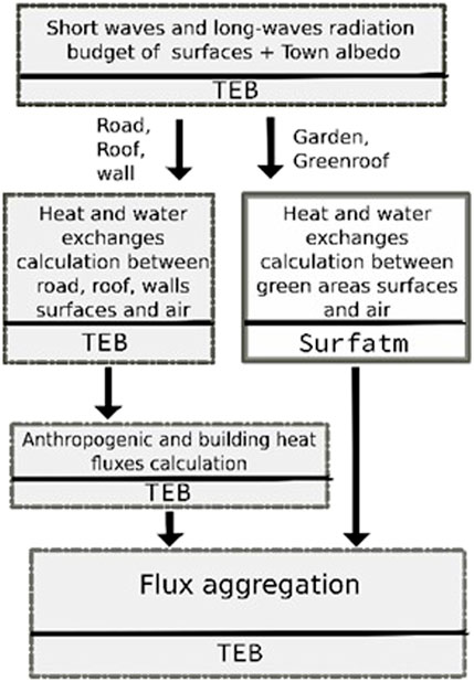
FIGURE 1. Diagram of inclusion of the Surfatm model into the TEB model.

The resistive scheme of the coupled TEB-Surfatm model is presented in Figure 2. Surfatm initially estimates the aerodynamic resistance between its reference height (i.e., the height for the input variables) and the top of the vegetation following the approach of Dyer and Hicks (1970). On the resistive scheme, the air resistance used in Surfatm for the garden (Ra_g) is similar to the one from TEB for the road (Ra_r). Air humidity and temperature inside the canyon used by Surfatm and TEB are the ones calculated at the previous time step. The displacement heights and roughness lengths for canopy and soil layers are fixed. Then Surfatm estimates net radiation (Rn), sensible and latent heat fluxes (H, LE), heat fluxes trough the soil (G), friction velocity (u*), drain and runoff over garden needed by TEB. On the green roof part, the same method is used excepted Surfatm uses the meteorological variables (air temperature and humidity) at the forcing level. Similarly to the aerodynamic resistances inside the canyon, the aerodynamic resistance between the forcing level and roof surface is calculated by TEB for both roof surfaces with and without vegetation (i.e., RaR and Ragr in Figure 2). Once every energy budget on each surface is simulated, TEB performs the final flux aggregation giving the estimated energy fluxes of the canyon (i.e., from walls, road, and garden) and the roofs (including both impervious and vegetated rooftop surfaces), the energy fluxes of the town (i.e., from road, garden, walls, and roofs), and the air temperature and humidity in the canyon that Surfatm needs as inputs in the next step.

FIGURE 2

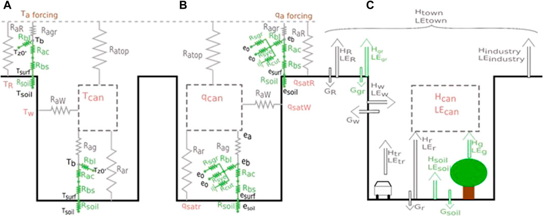
FIGURE 2. Resistive scheme of the TEB-Surfatm model for: (A) heat exchanges, (B) water vapour exchanges, and (C) energy budget. Ra_r, Ra_g, Ra_R, Ra_gr, Ra_w, R_bl, R_sgr, R_sye, R_cut, R_ac, R_bs, R_soil refer to aerodynamic resistances of the road, garden, roof, green roof, wall, leaf boundary layer resistance, the stomatal resistances of the green leaf and yellow leaf, the cuticular resistance, canopy aerodynamic resistance, soil boundary layer resistance, and soil resistance, respectively. e, q, qsat, T, H, LE, G refer to the water vapour partial pressure, specific humidity, saturation humidity, temperature, sensible and latent heat fluxes and the conductive flux, respectively. Brown scalars T_a forcing and q_a forcing are inputs. Grey and green resistances and fluxes refers to those calculated by TEB and Surfatm, respectively. Red and black scalars refer to those calculated by TEB and Surfatm, respectively.

Hence, the TEB-Surfatm model is able to provide results for the garden (i.e., trees, meadow and/or bare soil in the street), the canyon (garden + road), the roof (bare roof + green roof), and the town (canyon + roof) scales.

3 Model Evaluation

In order to evaluate the coupled TEB-Surfatm model, its outputs were compared with measurements performed during the COOLTREES project (Bournez 2018). The differences between model and measurements were analysed to understand and explain the discrepancies between estimated and experimental results.

3.1 Study Case

The experiment was carried out at the Jardin du Palais Universitaire in Strasbourg, France (48°35′04.4″N 7°45′48.2″E, 138 m altitude) from January 1^st, 2016 to December 31^th, 2016. The site consists in a vegetated place surrounded by some buildings. Its length and width are 220 and 90 m, respectively, and it is oriented at 112°. Meteorological variables and energy fluxes were measured by a 17 m height mast i.e, closed to the mean building height, thanks to several dedicated sensors. Samples were collected and stored every 15 min. A rotronic probe (HC2S3–Campbell) measured the air temperature and the relative humidity. A pyranometer CMP11 and a pyrgeometer CGR4 (Kipp and Zonen), directed downwards, measured the upwards solar and infrared radiations on the roof of a university building close to the park, respectively. A sonic anemometer (CSAT3 - Campbell) and a gas analyser (LI-7500A- LI-COR) measured the three wind speed components and the amount of water vapour in the air, respectively. LE and H were derived from Sonic data following the procedure proposed from Campbell. This place is a public garden with mainly grass, silver linden trees (Tilia tomentosa Moench), and some patches of bare soil (Figure 3).

FIGURE 3

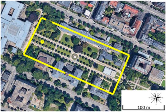
FIGURE 3. Aerial view of experimental site. The location of the measurement mast is shown with the yellow point. The area corresponding to the yellow rectangle is considered as an urban canyon.

3.2 Data Filtering Method

Data were filtered in order to remove outliers by absolute deviation around the median method (Leys et al., 2013). This method uses median absolute deviation (MAD) following Eq. 1 (Huber, 2004).

$MAD=1.4826\ast M_i\left(\left|x_j-M_j\left(x_j\right)\right|\right)(1)$

where M_j is the median of value at step t and the six observations around. M_i is the median of absolute difference between x_j and M_j. The value at step t is considered as an outlier and is removed from the dataset if it is outside interval spanning over the median plus/minus three MAD (Eq. 2).

$M_j-3MAD<x_i<M_j+3MAD(2)$

3.3 Footprint Analysis

The area considered by the micrometeorological flux measurements, i.e., the so-called “footprint”, is changing with time and depends on multiple factors such as wind direction and speed, surface roughness, and thermal stability (Burba and Anderson 2010). In order to ensure that the areas considered by both measurements and TEB-Surfatm model were similar, the footprint analysis using the Neftel model (Neftel et al., 2008) was performed. Its aim was to determine the area contributing to at least 80% of the measured fluxes. The MAD filter on this subdataset was applied and called Footprint_MAD.

3.4 TEB-Surfatm Configuration

3.4.1 Canyon Parameters

The experimental site is considered as a canyon with an average width of 63.2 m surrounded by buildings with an average height of 18 m and an average width of 17.4 m. Horizontal occupation fractions are shown in Table 1. The mean height of the trees is 9 m and that of the lawn is 0.1 m. Vegetated area is made up with 44% of trees, 34% of meadow and 22% of bare soil. Road included all impervious surfaces inside the canyon.

TABLE 1

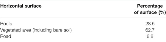
TABLE 1. Fractions of horizontal surfaces occupation.

3.4.2 Impervious Surfaces Configuration

Impervious surfaces parameters encompass radiative and thermal properties of roads, roofs, and walls. Most of parameters such as albedos, volumetric heat capacity, and thickness layers were chosen as proposed by Roupioz et al. (2018). There are based on field observations, measurements on this site, and documents about buildings constructed in this area at the same period. Values of materials’ emissivity materials came from the study of Landes et al. (2014) which used these values for the modelling work on this site. All parameters’ values are indicated in Table 2.

TABLE 2

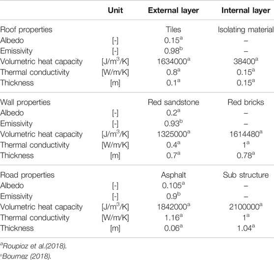
TABLE 2. TEB-Surfatm input parameters for impervious surfaces.

3.4.3 Vegetated Surfaces Parameters

The vegetated surfaces in the modelling approach consist in the soil layer and the vegetation layer. The latter, by using a big leaf approach, must be representative of both trees and grass on the experimental site. The parameters concerning the whole vegetated surface and the vegetation layer were determined by weighted averaging of the individual parameters of soil and/or trees and grass (Masson, 2000; Lemonsu et al., 2012) i.e.:

$P_{veg\_surface}={\alpha }_{grass}{P}_{grass}+{\alpha }_{tree}{P}_{tree}+{\alpha }_{soil}{P}_{soil}(3)$

Or

$P_{veg}={\alpha }_{grass\_2}{P}_{grass}+{\alpha }_{tree\_2}{P}_{tree}(4)$

where α_grass, α_tree, α_soil are the fractions of grass, trees, and bare soil of vegetated surfaces (0.34, 0.44, and 0.22, respectively) and α_{grass_2} and α_{tree_2} are the fractions of grass and trees of vegetation (0.44 and 0.56, respectively). P_grass, P_tree, P_soil are the parameters of grass, trees, and soil, respectively. The parameters used in the model concerning the whole vegetated surface were therefore determined from Eq. 3 while those concerning the vegetation layer were determined from Eq. 4. The individual parameters for soil, trees, and grass as well as the final result for model input are indicated in the Table 3.

TABLE 3

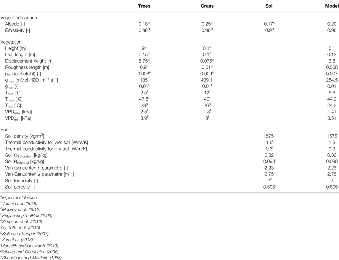
TABLE 3. Parameters for trees, grass and soil, and final parameters retained for model input.

4 Results and Discussion

4.1 Meteorological Conditions and Measured Fluxes

The annual trend of global radiation (Rg), in 2016, followed a typical pattern with minimum values during winter (mean daily values around 10 W/m²), increased during spring to reach a maximum in summer, and then decreased during autumn and winter. Mean daily Rg exhibited strong day-to-day variations, especially in summer (from around 100 W/m² to 350 W/m²) due to the interplay of cloudy and sunny periods (Figure 4A). At the daily scale, Rg increased from sunrise to reach its maximum (around 410 W/m² on average) at noon, and then decreased during the afternoon to reach its nocturnal value i.e., 0 W/m² (Figure 4B). The mean annual (±standard deviation) Rg was 130 ± 90 W/m², and 1^st and 3^rd quartiles were 40 W/m² and 200 W/m², respectively. Air temperature (Ta) and relative humidity (RH) were anti-correlated. At the daily scale, Ta increased from early morning to reach its maximum (around 18°C on average) in early afternoon and then decreased to its nocturnal value (around 12°C on average). RH followed the opposite trend by decreasing in the morning to around 60% on average in early afternoon before increasing to its maximum nocturnal value (around 90% on average) (Figure 4D). At the yearly scale, Ta followed the same pattern as Rg with minimum daily temperature around -4°C in winter and maximum around 28°C in summer. RH followed the converse annual trend and decreased from around 100% during winter to around 44% in summer before increasing during autumn (Figure 4C). As for Rg, RH and Ta exhibited large day-to-day variations i.e., drier and warmer days during sunny periods and wetter and colder days during cloudy periods. Mean annual Ta and RH were 12 ± 7°C (1^st and 3^rd quartiles equal to 6°C and 19°C) and 75 ± 13% (1^st and 3^rd quartiles equal to 65 and 85%), respectively. Over the whole year, rainfall accounted for 730 mm. These events occurred regularly, with 168 rainy days, with on average 9 ± 11 mm/day. Overall, it was dry in winter and wet in summer, with the wettest period from April to June. Indeed some particularly rainy days occurred during this period with daily rain accounting for up to 30 mm. The period from June to September was dry with only sparse rainy days (Figure 4G). The daily-mean wind speed varied between 0 m/s to 7 m/s and direction was mostly oriented to North-East (15–45°) and South (165–195°). The highest wind speeds occurred in the West-Southwest and East-Northeast directions (Figure 4H). Overall, the meteorological conditions were representative of the continental climate.

FIGURE 4

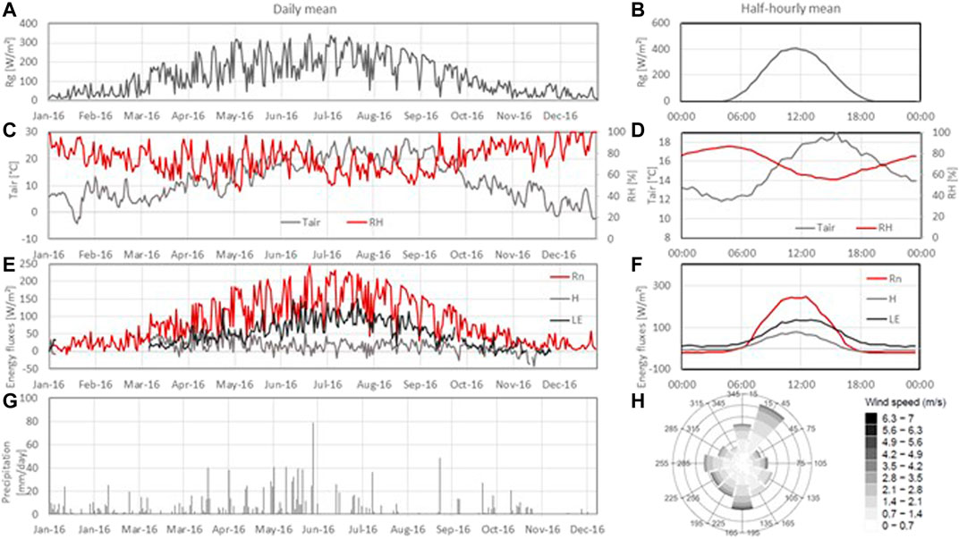
FIGURE 4. Daily (left) and half-hourly (right) means of (A,B) global radiation (Rg), (C,D) relative humidity (RH) (red line) and air temperature (Tair) (grey line), and (E,F) net radiation (Rn) (red line), sensible heat flux (H) (grey line) and latent heat flux (LE) (black line). (G) Daily cumulated precipitation and (H) wind rose of half-hourly mean wind speed.

Daily means and mean half-hourly values of the measured net radiation (Rn) and sensible (H) and latent (LE) heat fluxes are represented in Figures 4E,F, respectively. The MAD filter (see Section 3.2) was applied on both H and LE data. At the daily scale, Rn, H, and LE followed the same dynamics: they remained stable during nighttime, increased during the morning to peak to their maximum at noon, and decreased to their nocturnal values during the afternoon. Maximum half hourly values were on average 300 W/m², 140 W/m² and 80 W/m² for Rn, LE, and H, respectively. During nighttime, Rn and H were both slightly negative while LE remained positive (Figure 4F). At the yearly scale, Rn followed the same seasonal and day-to-day dynamics as Rg. Mean daily Rn varied between around -25 W/m² and +25 W/m² during winter and between 75 and 190 W/m² during summer. Mean daily H did not exhibited seasonal evolution and ranged from -40 W/m² to 80 W/m², whereas mean daily LE increased from 0 W/m² during winter to 50–150 W/m² during summer and then decreased during autumn in link with the phenological development and physiological activity of the vegetation present in the site (Figure 4E).

4.2 Comparison Between Measured and Modelled Energy Fluxes

In order to validate the TEB-Surfatm model, modelled energy fluxes were compared with the in-situ measurements which were filtered with the MAD method (see Section 3.2) i.e., by removing outliers.

Convective flux measurements were performed with the eddy-covariance method (see Section 3.1) i.e., a micrometeorological method providing integrated flux estimates on a certain area. This area, the so-called “footprint”, changes according to surface parameters (e.g., roughness or measurement height) and micrometeorological variables (e.g., wind direction and speed or atmospheric stability). Yet, TEB-Surfatm provides energy fluxes at three different scales: the vegetated area (including bare soil noted hereafter “Garden”), the road + garden area (hereafter “Canyon”), and the whole city including road, garden, walls, and roofs surfaces (hereafter “Town”). As a first approach, model outputs at these three different scales were compared to measurements in order to determine which scale was the most relevant for the comparison of modelled and measured fluxes. Four statistical indicators were used to assess these comparisons: the equation of the regression line, the Root Mean Square Error (RMSE), the bias, and the Mean Absolute Percentage Error (MAPE). The results are presented in Figure 5; Table 4.

FIGURE 5

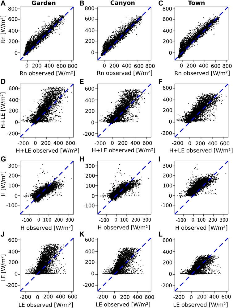
FIGURE 5. Comparison of measured and modelled (A–C) net radiation (Rn), (D–F) total conductive heat fluxes (H + LE), (G–I) sensible heat fluxes (H), and (J–L) latent heat fluxes (LE) modelled at the garden (first column), canyon (second column) and town (third column) scales.

TABLE 4

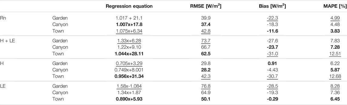
TABLE 4. Equation of the regression line, Root Mean Square Error (RMSE), Bias, and Mean Absolute Percentage Error (MAPE) between the predicted fluxes at the garden, canyon, and town scales and the measured fluxes. For each energy flux, the best and worst values of the statistical indicators according to the output scale are indicated in bold and underlined, respectively.

Modelled and measured Rn exhibited a quite good agreement whatever the scale in model outputs considered i.e., garden (Figure 5A), canyon (Figure 5B), or town (Figure 5C) scale. However, the outputs at the canyon scale exhibited the best agreement with the measurements for both the regression line and the RMSE. Despite the best agreement with the measurements considering the bias and the MAPE statistical indicators for the town scale, this last also revealed the worst agreement considering the regression line and the RMSE. The Rn modelled at the garden scale exhibited the worst agreement with measurements considering bias and MAPE indicators (Table 4).

For the total convective heat fluxes (i.e., H + LE), although the fluxes estimated by the TEB-Surfatm model exhibited a quite good agreements with the measurements whatever the scale considered (Figures 5D–F), the best regression line was found for the fluxes modelled at the town scale which also exhibited the best RMSE but the worst bias and MAPE. On the contrary, total convective heat fluxes modelled at the garden scale exhibited the worst agreement considering regression line and RMSE. Those modelled at the canyon scale revealed the best agreement for both bias and MAPE (Table 4). Considering only latent heat fluxes, it was clear that the modelled LE at the town scale fitted the best with measurements since the best values for the four statistical indicators were found at this scale, and the four worst at the garden scale (Table 4). For the sensible heat flux, results were less clear: the town scale obtained the best regression but the worst values for the three other statistical indicators, the garden scale exhibited the worst regression but the best bias, and the canyon scale revealed the best values for RMSE and MAPE (Table 4).

Considering the whole results and statistical indicators, modelled fluxes at the canyon scale provided six best values for the statistical indicators, ten intermediates, and no worst values, while it was one best value, six intermediates, and nine worst values at the garden scale, and nine best, no intermediates, and seven worst values at the town scale (Table 4). These findings suggested that the canyon scale was overall the best modelling scale for the comparison with measurements. In addition, the fluxes were measured close to the mean building height. In this case it is a reasonable hypothesis to suppose that the fluxes mainly originated from the road and garden surfaces i.e., at the canyon scale. Therefore, fluxes are studied at the canyon scale in the following parts.

The partitioning of total convective heat fluxes in H and LE exhibited underestimation and overestimation of the measurements, respectively. Many issues could explain that finding such as the impact of the footprint from measurements or some missing or not well represented processes in the TEB-Surfatm model. These issues are explored in the following.

4.3 Residual Analysis

As stated previously, only the modelled fluxes at the canyon scale are considered. The aim of this part is to investigate the discrepancies between the modelled and measured fluxes. Hence, the residues, as the difference between measured and modelled values (i.e., positive when the observed values are larger than the predicted ones, and conversely), were estimated. The data were filtered with the MAD method (see Section 3.2; noted hereafter “MAD”), and also by including the filter based on the measurement footprint (noted hereafter “Footprint_MAD”). This latter consisted in keeping only the data for which at least 80% of the measured flux originated from maximum 200 m (i.e., the garden length) from the mast.

The residues were first analysed as a function of the deciles of measured energy fluxes. The Figures 6A,B show the boxplots of the residues according to the deciles of the measurements for H and LE, respectively. Typically, 1^st decile corresponds to low flux magnitude (i.e., during nighttime and/or winter) and 10^th decile corresponds to maximum flux magnitude (i.e., at noon and/or summer). Both results with MAD and Footprint_MAD filters are presented. Results of the pairwise comparisons are also shown: a letter shared between two or more boxplots indicated no significant differences, and two boxplots that do not share a common letter are significantly different.

FIGURE 6

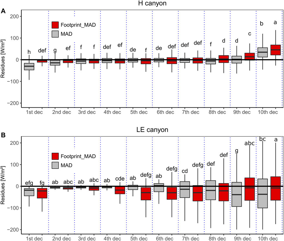
FIGURE 6. Boxplots of the residues filtered with the MAD (grey) and Footprint_MAD (red) methods for each decile of the measurements for (A) H and (B) LE fluxes. Are also indicated the results from the pairwise comparison Turkey’s HSD statistical test (see text for details and explanations for the interpretation).

The modelled and measured H fluxes presented a quite good agreement most of the time, residues boxplots being centred and closed to zero from 3^rd to 8^th measured H deciles (Figure 6A). Yet, considering the footprint for this measurement range did not improve the model accuracy since overall no significant differences where observed between residues with MAD filter and with Footprint_MAD filter for 3^rd to 7^th deciles of measured H. However, the model overestimated (i.e., negative values of the residues) H fluxes for low H values (i.e., 1^st and 2^nd deciles) (Figure 6A). In this case, applying the Footprint_MAD filter clearly and significantly improved the model/measures agreement. For the highest values of measured H (i.e., 10^th and to a less extend 9^th deciles), the model underestimated (i.e., positive values of the residues) the fluxes (Figure 6A). Applying the Footprint_MAD filter induced an even low but significant worst agreement with measurements (residues median, 1^st, and 3^rd quartiles equal to 46 W/m², 22 W/m², and 69 W/m², respectively) than with the MAD filter (residues median, 1^st, and 3^rd quartiles equal to 35 W/m², 12 W/m², and 56 W/m², respectively) (Figure 6A), suggesting that the measurement footprint was not the only reason for model overestimation. It will be explored in the following sections.

For the lowest LE values (i.e., 1^st decile of the measurements), the model strongly overestimated (i.e., negative values of the residues) the measurements. When LE fluxes were quite low (i.e., 2^nd and 3^rd deciles of measurements), the model agreed well with the measurements: residues were closed to zero whatever the filter (MAD or Footprint_MAD) considered. From 4^th to 10^th deciles of the measurements, the model globally overestimated the measured LE fluxes and its accuracy decreased when measured LE increased (i.e., the interquartile range (IQR) of the residues boxplots increased) (Figure 6B). Moreover, although applying the Footprint_MAD filter clearly improved the model/measures comparison for the highest values of LE (i.e., 9^th and 10^th deciles of measurements), it led to worst agreement for intermediates values of LE (i.e., 4^th, 5^th, and 6^th deciles of measurements) (Figure 6B).

Hence, the ability of the TEB-Surfatm model to estimate H and LE fluxes varied according to the flux magnitude. The model reproduced well H fluxes excepted for very high H fluxes and overestimated overall LE fluxes. The discrepancies partially originated from the measurement footprint: the area contributing to the measured flux could be larger than the area considered by the TEB-Surfatm model. However, the measurement footprint did not explain all the differences between measured and modelled fluxes. Other issues, such as biophysical processes not well taken into account could not be discarded. Correlations between residues and measured meteorological variables (global radiation, air humidity, wind direction and speed, soil temperatures, and soil water content) were tested (data not shown) but no significant correlation were established. In the following, the temporal (i.e., daily and seasonal) and spatial variabilities of the residues were explored to explain the differences between model and measured fluxes.

4.4 Temporal and Spatial Analysis of the Residues

The two-hours residues boxplots for H and LE fluxes with MAD and Footprint_MAD filters are presented for spring (Figures 7A,B), summer (Figures 7C,D), and autumn (Figures 7E,F) seasons.

FIGURE 7

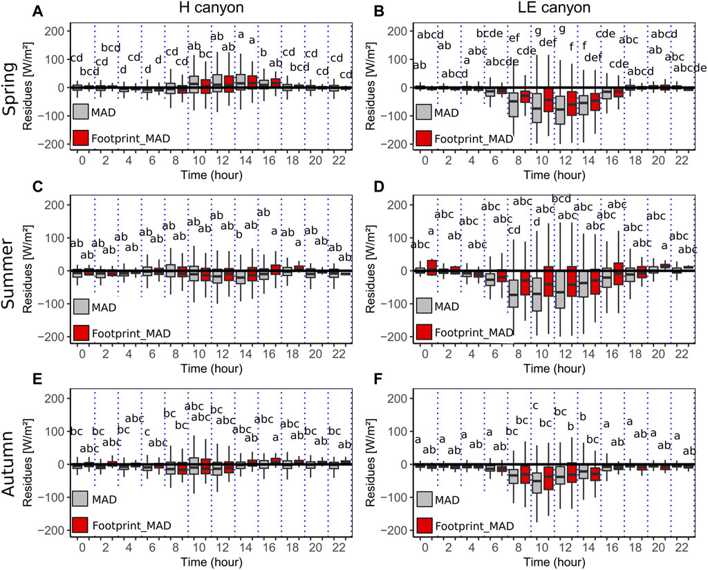
FIGURE 7. Two-hours boxplots of the residues filtered with the MAD (grey) and Footprint_MAD (red) methods for H and LE fluxes during (A,B) spring, (C,D) summer, and (E,F) autumn, respectively. Are also indicated the results from the pairwise comparison Turkey’s HSD statistical test (see text for details and explanations for the interpretation).

For H fluxes, the IQR of the residues exhibited a clear daily variation. It was weak during nighttime, increased during the morning, peaked to its maximum at noon, and decreased during the afternoon to the minimum IQR. This trend occurred whatever the season considered (Figures 7A,C,E). Hence, the absolute error between measured and modelled H fluxes varied throughout the day, but it must be kept in mind that the flux magnitude also varied with a maximum near noon (see Section 4.1 and Figure 4F). Hence, in terms of relative error, the performance of the TEB-Surfatm model was overall constant at the daily scale. Most often a slightly better agreement (median closer to zero, smaller IQR) is observed with the Footprint_MAD filter. Yet, even if it was quite weak, it must be noted that the TEB-Surfatm model slightly underestimated (i.e., positive residues) the H fluxes during spring (Figure 7A) and slightly overestimated (i.e., negative residues) the H fluxes during summer (Figure 7C) and autumn (Figure 7E).

As for the LE fluxes, the IQR of the residues exhibited a similar and clear daily variation for all seasons (Figures 7B,D,F) i.e., the absolute error of the model increased with the magnitude of the LE flux. Contrary to H fluxes, the model systematically overestimated the LE flux measurements at the two-hours time scale. Nevertheless, considering the measurement footprint improved the ability of the model to reproduce the measurements. With the Footprint_MAD filter, the residues boxplots were systematically closer to zero, but no dependence on the season occurred. Yet, it overall did not change the IQR of the residues boxplots.

The footprint depends notably on wind direction, therefore, the ‘measurement area’ is not centred on the mast and can largely differ from the ‘modelling area’. In order to investigate that issue, a method of bivariate interpolation and smooth surface fitting was used to present the residues values at points distributed in a x-y plane determined by distances and directions from the mast (Akima, 1978, 1996). These results are presented in Figure 8. Each pixel delimits the upwind distance from the mast for which 80% of the measured flux originated from. For each pixel, estimated residues was sorted in three categories for H (Figure 8A) and LE (Figure 8B).

FIGURE 8

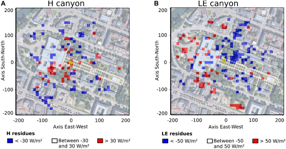
FIGURE 8. Spatial distribution of the residues for (A) H and (B) LE fluxes. The area considered by the model is indicated by the grey rectangle and the measurement mast by the yellow dot.

This representation allows an interpretation of the differences between the model and measurements according to distance and direction from the mast i.e., the footprint of the measurements.

The H fluxes were underestimated (i.e., residues larger than 30 W/m²) by the model when the footprint was very closed to the mast, extended at 50 m south from the mast, and 80–90 m west-south-west from the mast. Model overestimation (i.e., residues lower than -30 W/m²) mainly occurred when the footprint extended to up to 100 m from the southern, western, and northern directions. However, when the measurements footprint was in the canyon considered by the TEB-Surfatm model, neither over- nor underestimation was observed (i.e., residues between -30 W/m² and 30 W/m²) (Figure 8A).

The modelled LE fluxes were underestimated (i.e., residues larger than 50 W/m²) mainly when the measurement footprint originated from south-south-west to north-west directions, and overestimated (i.e., residues lower than -50 W/m²) when it originated from north-east to east directions from the mast. The modelled LE fluxes exhibited a good agreement with measurements (i.e., residues between -50 W/m² and 50 W/m²) when the measurements footprint was in the canyon, except for the area close to the mast in the east direction (Figure 8B).

Hence, the variability of the model accuracy depended on the measurement footprint in link with the heterogeneity of the site characteristics. While the measurement footprint fitted with the area characteristics considered by the TEB-Surfatm model, the modelled H and LE fluxes presented a good agreement with the measurements. It proved the ability of the coupled model to estimate the energy fluxes in urban area, accounting for impervious and vegetated surfaces. The underestimation and overestimation in the western area from the mast for H and LE fluxes, respectively, could be attributed to a more important fraction of impervious surface than what it was considered in the model. Indeed, this zone consisted in mainly a built-up area (Figure 3). Therefore, the evapotranspiration is very weak and most of the energy received by the surface would be dissipated through H flux compared to a vegetated area (Gunawardena et al., 2017; Chrysoulakis et al., 2018). The model overestimation of LE fluxes when the footprint originated from north-north-east and east directions could also be attributed to a difference between the site and modelled characteristics. Indeed, the amount of trees in these areas is larger than the amount considered in the modelled area (Figure 3). Since the maximum stomatal conductance (g_max) is three times larger for grass than for tree (Table 3), the larger amount of grass in the model can lead to model overestimation of the LE fluxes in these areas. That issue was also observed in previous studies (e.g., Wang et al., 2012; Zou et al., 2021). For instance, Litvak et al. (2014) reported that the evapotranspiration of a grass plot was between +50% and +100% larger than a mixed grass and trees plot in summer.

5 Conclusion

The TEB and Surfatm models were coupled in order to estimate energy fluxes in urban areas, accounting for urban green spaces. The coupled TEB-Surfatm model was evaluated against measurements performed in Strasbourg, France, within an urban park composed by grass and trees. The model was able to reproduce the energy fluxes, but its performance varied. The variability of the model accuracy depended on the measurement footprint in link with the heterogeneity of the site characteristics: while the measurement footprint fitted with the area characteristics considered by the TEB-Surfatm model, the modelled H and LE fluxes presented a good agreement with the measurements. In the other cases, some overestimation and underestimation occurred, in link with different fractions of impervious surfaces or green spaces. Hence, strong attention must be given to the model/measure comparisons especially in heterogeneous urban sites, by considering the accordance between the model area and the measurement footprint to avoid erroneous conclusions concerning the model validation.

UHI mitigation, especially in the context of global warming, is of particular importance for citizen comfort and health. To this aim, stakeholders need information on the potential of green spaces to improve the city sustainability. Therefore, the TEB-Surfatm model can be used for the quantification of the impact of urban greening on the urban heat island effect.

Last but not least, the Surfatm model was initially developed for the modelling of pollutant exchanges between the atmosphere and the vegetation. Since the enhancement of air quality in urban area is of particular interest for citizen health (Shang et al., 2013; Andrea Rodriguez-Villamizar et al., 2018; Eisenman et al., 2019), finding solutions to promote atmospheric pollutant removal are required. The TEB-Surfatm model would be able to quantify the impact of urban vegetation of pollutant deposition, and therefore on air quality. This work, i.e., the inclusion of pollutant deposition in the TEB-Surfatm model, will be the next step of the model development.

Data Availability Statement

The raw data supporting the conclusions of this article will be made available by the authors, without undue reservation.

Author Contributions

SL coupled and run the TEB-Surfatm model compared the results with measurements. SL and PS wrote the first draft of the paper. DF, EP, and PS supervised the whole modelling work. GN, PK, TA, MS conducted the field measurements and data processing. JC was in charge of radiometers and sonic anemometers deployement and maintenance, and data centralization. All the authors contributed to the final version of the paper and to data interpretation.

Funding

This modelling work was supported by a grant from Vinci through the Lab Recherche-Environnement Vinci-ParisTech. The experimental dataset collection was part of the COOLTREES project (ANR-17-CE22-0012) funded by the French National Research Agency (ANR). This work benefited from the French state aid managed by the ANR under the “Investissements d’avenir” programme with the reference ANR-16-CONV-0003.

Conflict of Interest

The authors declare that the research was conducted in the absence of any commercial or financial relationships that could be construed as a potential conflict of interest.

Publisher’s Note

All claims expressed in this article are solely those of the authors and do not necessarily represent those of their affiliated organizations, or those of the publisher, the editors and the reviewers. Any product that may be evaluated in this article, or claim that may be made by its manufacturer, is not guaranteed or endorsed by the publisher.

Acknowledgments

Warm thanks to Francis Bruckmann (Faculté de Géographie et Université de Strasbourg), Raphaël Luhahe (Université de Strasbourg) and Philippe Obrecht (Chief gardener- Université de Strasbourg) for their technical assistance with fieldwork and to the University of Strasbourg for all the authorizations to access the jardin du Palais Universitaire.

References

Akbari, H., Pomerantz, M., and Taha, H. (2001). Cool Surfaces and Shade Trees to Reduce Energy Use and Improve Air Quality in Urban Areas. Solar Energy 70, 295–310. doi:10.1016/S0038-092X(00)00089-X

CrossRef Full Text | Google Scholar

Akima, H. (1996). Algorithm 761: Scattered-Data Surface Fitting that Has the Accuracy of a Cubic Polynomial. TOMS 22 (3), 362–371. doi:10.1145/355780.355786

CrossRef Full Text | Google Scholar

Akima, H. (1978). A Method of Bivariate Interpolation and Smooth Surface Fitting for Irregularly Distributed Data Points. ACM Trans. Math. Softw. 4 (2), 148–159. doi:10.1145/355780.355786

CrossRef Full Text | Google Scholar

Alchapar, N., Correa, É., and Cantón, M. A. (2014). Classification of Building Materials Used in the Urban Envelopes According to Their Capacity for Mitigation of the Urban Heat Island in Semiarid Zones. doi:10.1016/j.enbuild.2013.10.012

CrossRef Full Text | Google Scholar

Alexandri, E., and Jones, P. (2008). Temperature Decreases in an Urban Canyon Due to Green Walls and Green Roofs in Diverse Climates. Building Environ. 43 (4), 480–493. doi:10.1016/j.buildenv.2006.10.055

CrossRef Full Text | Google Scholar

Arnfield, A. J. (2003). Two Decades of Urban Climate Research: A Review of Turbulence, Exchanges of Energy and Water, and the Urban Heat Island. Int. J. Climatol. 23 (1), 1–26. doi:10.1002/joc.859

CrossRef Full Text | Google Scholar

Berwal, S., Kumar, D., Pandey, A. K., Singh, V. P., Kumar, R., and Kumar, K. (2016). Dynamics Of Thermal Inertia Over Highly Urban City: A Case Study Of Delhi. Proceedings Volume 10008, Remote Sensing Technologies and Applications in Urban Environments, 100080E. doi:10.1117/12.2241741

CrossRef Full Text | Google Scholar

Bornstein, R., and Lin, Q. (2000). Urban Heat Islands and Summertime Convective Thunderstorms in Atlanta: Three Case Studies Atmos. Environ 34, 507–516. doi:10.1016/S1352-2310(99)00374-X

CrossRef Full Text | Google Scholar

Bournez, E. (2018). “Etude Du Rôle de La Végétation Dans La Création de Microclimats Urbains : Approche Combinée de Mesures et de Modélisations à Différentes Échelles,”. PhD thesis (Strasbourg: Université de Strasbourg).

Google Scholar

Bouyer, J. (2009). “Modélisation et simulation des microclimats urbains - Étude de l’impact de l’aménagement urbain sur les consommations énergétiques des bâtiments,”. PhD thesis (Nantes: Université de Nantes).

Google Scholar

Bouyer, J., Musy, M., and Huang, Y. (2009). Cities and Climate, Chapter 5: Mitigating Urban Heat Island Effect by Urban Design: Forms and Materials. Washington DC: World Bank, 164–181.

Google Scholar

Bowler, D. E., Buyung-Ali, L., Knight, T. M., and Pullin, A. S. (2010). Urban Greening to Cool Towns and Cities: A Systematic Review of the Empirical Evidence. Landscape Urban Plann. 97 (3), 147–155. doi:10.1016/j.landurbplan.2010.05.006

CrossRef Full Text | Google Scholar

Bruse, M., and Fleer, H. (1998). Simulating Surface-Plant-Air Interactions inside Urban Environments with a Three Dimensional Numerical Model. Environ. Model. Softw. 13, 373–384. doi:10.1016/S1364-8152(98)00042-5

CrossRef Full Text | Google Scholar

Burba, G., and Anderson, D. (2010). A Brief Practical Guide to Eddy Covariance Flux Measurements: Principles and Workflow Examples for Scientific and Industrial Applications. LI-COR Biosciences, 212. doi:10.13140/RG.2.1.1626.4161

CrossRef Full Text | Google Scholar

Choudhury, B. J., and Monteith, J. L. (1988). A Four-Layer Model for the Heat Budget of Homogeneous Land Surfaces. Q.J R. Met. Soc. 114 (480), 373–398. doi:10.1002/qj.49711448006

CrossRef Full Text | Google Scholar

Chrysoulakis, N., Grimmond, S., Feigenwinter, C., Lindberg, F., Gastellu-Etchegorry, J.-P., Marconcini, M., et al. (2018). Urban Energy Exchanges Monitoring from Space. Sci. Rep. 8 (1), 11498. doi:10.1038/s41598-018-29873-x

PubMed Abstract | CrossRef Full Text | Google Scholar

Dimoudi, A., and Nikolopoulou, M. (2003). Vegetation in the Urban Environment: Microclimatic Analysis and Benefits. Energy and Buildings 35, 69–76. doi:10.1016/S0378-7788(02)00081-6

CrossRef Full Text | Google Scholar

Duneier, M. (2006). Ethnography, the Ecological Fallacy, and the 1995 Chicago Heat Wave. Am. Sociol. Rev. 71, 679–688. doi:10.1177/000312240607100408

CrossRef Full Text | Google Scholar

Dyer, A. J., and Hicks, B. B. (1970). Flux-gradient Relationships in the Constant Flux Layer. Q.J R. Met. Soc. 96 (410), 715–721. doi:10.1002/qj.49709641012

CrossRef Full Text | Google Scholar

Eisenman, T. S., Churkina, G., Jariwala, S. P., Kumar, P., Lovasi, G. S., Pataki, D. E., et al. (2019). Urban Trees, Air Quality, and Asthma: An Interdisciplinary Review. Landscape Urban Plann. 187, 47–59. doi:10.1016/j.landurbplan.2019.02.010

CrossRef Full Text | Google Scholar

Emmanuel, R., and Fernando, H. (2007). Urban Heat Islands in Humid and Arid Climates: Role of Urban Form and thermal Properties in Colombo, Sri Lanka and Phoenix, USA. Clim. Res. 34, 241–251. doi:10.3354/cr00694

CrossRef Full Text | Google Scholar

Engineering ToolBox, (2003). Emissivity Coefficient Materials. Available at: https://www.engineeringtoolbox.com/emissivity-coefficients-d_447.html [Accessed 19 Feb 2021].

Google Scholar

Feyisa, G. L., Dons, K., and Meilby, H. (2014). Efficiency of Parks in Mitigating Urban Heat Island Effect: An Example from Addis Ababa. Landscape Urban Plann. 123, 87–95. doi:10.1016/j.landurbplan.2013.12.008

CrossRef Full Text | Google Scholar

Gillner, S., Vogt, J., Tharang, A., Dettmann, S., and Roloff, A. (2015). Role of Street Trees in Mitigating Effects of Heat and Drought at Highly Sealed Urban Sites. Landscape Urban Plann. 143, 33–42. doi:10.1016/j.landurbplan.2015.06.005

CrossRef Full Text | Google Scholar

Gunawardena, K. R., Wells, M. J., and Kershaw, T. (2017). Utilising Green and Bluespace to Mitigate Urban Heat Island Intensity. Sci. Total Environ. 584-585, 1040–1055. doi:10.1016/j.scitotenv.2017.01.158

PubMed Abstract | CrossRef Full Text | Google Scholar

Hamdi, R., and Masson, V. (2008). Inclusion of a Drag Approach in the Town Energy Balance (TEB) Scheme: Offline 1D Evaluation in a Street Canyon. J. Appl. Meteorology Climatology 47 (10), 2627–2644. doi:10.1175/2008JAMC1865.1

CrossRef Full Text | Google Scholar

Harlan, S. L., and Ruddell, D. M. (2011). Climate Change and Health in Cities: Impacts of Heat and Air Pollution and Potential Co-benefits from Mitigation and Adaptation . Curr. Opin. Environ. Sustainability 3, 126–134. doi:10.1016/j.cosust.2011.01.001

CrossRef Full Text | Google Scholar

Huber, P. J. (2004). Robust Statistics. New York: John Wiley & Sons.

Google Scholar

Imbert, C., Bhattacharjee, S., and Tencar, J. (2018). “Simulation of Urban Microclimate with SOLENE-Microclimat - an Outdoor Comfort Case Study,” in Proceedings of the symposium on simulation for architecture and urban design, Delft, the Netherlands, June 05-07. (Society for Computer Simulation International), 1–8. doi:10.22360/simaud.2018.simaud.026

CrossRef Full Text | Google Scholar

Johnson, G. T., Oke, T. R., Lyons, T. J., Steyn, D. G., Watson, I. D., and Voogt, J. A. (1991). Simulation of Surface Urban Heat Islands under ?IDEAL? Conditions at Night Part 1: Theory and Tests against Field Data. Boundary-layer Meteorol. 56 (3), 275–294. doi:10.1007/BF00120424

CrossRef Full Text | Google Scholar

Kastendeuch, P. P., Najjar, G., and Colin, J. (2017). Thermo-radiative Simulation of an Urban District with LASER/F. Urban Clim. 21, 43–65. doi:10.1016/j.uclim.2017.05.003

CrossRef Full Text | Google Scholar

Kumar, R., and Kaushik, S. C. (2005). Performance Evaluation of Green Roof and Shading for Thermal Protection of Buildings. Building Environ. 40, 1505–1511. doi:10.1016/j.buildenv.2004.11.015

CrossRef Full Text | Google Scholar

Landes, T., Hayot, C., Najjar, G., Kastendeuch, P., Saudreau, M., Colin, J., et al. (2014). Modélisation 3D d’arbre pour comprendre le climat urbain. Un projet multidisciplinaire ambitieux. Revue XYZ, 141. 4e trimestre 2014, 55–62.

Google Scholar

Lemonsu, A., Masson, V., Shashua-Bar, L., Erell, E., and Pearlmutter, D. (2012). Inclusion of Vegetation in the Town Energy Balance Model for Modelling Urban green Areas. Geosci. Model. Dev. 5 (6), 1377–1393. doi:10.5194/gmd-5-1377-2012

CrossRef Full Text | Google Scholar

Leys, C., Ley, C., Klein, O., Bernard, P., and Licata, L. (2013). Detecting Outliers: Do Not Use Standard Deviation Around the Mean, Use Absolute Deviation Around the Median. J. Exp. Soc. Psychol. 49 (4), 764–766. doi:10.1016/j.jesp.2013.03.013

CrossRef Full Text | Google Scholar

Li, C., Zhou, J., Cao, Y., Zhong, J., Liu, Y., Kang, C., et al. (2014). Interaction between Urban Microclimate and Electric Air-Conditioning Energy Consumption during High Temperature Season. Appl. Energ. 117, 149–156. doi:10.1016/j.apenergy.2013.11.057

CrossRef Full Text | Google Scholar

Lichiheb, N., Personne, E., Bedos, C., and Barriuso, E. (2014). Adaptation of a Resistive Model to Pesticide Volatilization from Plants at the Field Scale: Comparison with a Dataset. Atmos. Environ. 83, 260–268. doi:10.1016/j.atmosenv.2013.11.004

CrossRef Full Text | Google Scholar

Litvak, E., Bijoor, N. S., and Pataki, D. E. (2014). Adding Trees to Irrigated Turfgrass Lawns May Be a Water-Saving Measure in Semi-arid Environments. Ecohydrology 7 (5), 1314–1330. doi:10.1002/eco.1458

CrossRef Full Text | Google Scholar

Liu, Z., He, C., Zhou, Y., and Wu, J. (2014). How Much of the World’s Land Has Been Urbanized, Really? A Hierarchical Framework for Avoiding Confusion. Landscape Ecol. 29. doi:10.1007/s10980-014-0034-y

CrossRef Full Text | Google Scholar

Martilli, A., Clappier, A., and Rotach, M. W. (2002). An Urban Surface Exchange Parameterisation for Mesoscale Models. Boundary-Layer Meteorology 104 (2), 261–304. doi:10.1023/a:1016099921195

CrossRef Full Text | Google Scholar

Masson, V. (2000). A Physically-Based Scheme for the Urban Energy Budget in Atmospheric Models. Boundary-Layer Meteorology 94 (3), 357–397. doi:10.1023/a:1002463829265

CrossRef Full Text | Google Scholar

Masson, V., Grimmond, C. S. B., and Oke, T. R. (2002). Evaluation of the Town Energy Balance (TEB) Scheme with Direct Measurements from Dry Districts in Two Cities. J. Appl. Meteorology 41 (10), 1011–1026. doi:10.1175/1520-0450(2002)041<1011:EOTTEB>2.0.CO;2

CrossRef Full Text | Google Scholar

Mcevoy, A., Markvart, T., and Castañer, L. (2012). Practical Handbook of Photovoltaics. Fundamentals and Applications. 2nd edn. Waltham, MA: Academic Press. doi:10.1016/C2011-0-05723-X

CrossRef Full Text | Google Scholar

Memon, R. A., Leung, D. Y. C., and Liu, C.-H. (2009). An Investigation of Urban Heat Island Intensity (UHII) as an Indicator of Urban Heating. Atmos. Res. 94 (3), 491–500. doi:10.1016/j.atmosres.2009.07.006

CrossRef Full Text | Google Scholar

Middel, A., Häb, K., Brazel, A. J., Martin, C. A., and Guhathakurta, S. (2014). Impact of Urban Form and Design on Mid-afternoon Microclimate in Phoenix Local Climate Zones. Landscape Urban Plann. 122, 16–28. doi:10.1016/j.landurbplan.2013.11.004

CrossRef Full Text | Google Scholar

Monteith, J. L., and Unsworth, M. H. (2013). Principles of Environmental Physics: Plants, Animals, and the Atmosphere. 4th edn. Amsterdam; Boston: Elsevier/Academic Press.

Google Scholar

Neftel, A., Spirig, C., and Ammann, C. (2008). Application and Test of a Simple Tool for Operational Footprint Evaluations. Environ. Pollut. 152 (1523), 644–652. doi:10.1016/j.envpol.2007.06.062

PubMed Abstract | CrossRef Full Text | Google Scholar

Noilhan, J., and Mahfouf, J.-F. (1996). The ISBA Land Surface Parameterisation schemeThe ISBA Land Surface Parameterisation Scheme. Global and Planetary Change. Glob. Planet. Change 13, 145–159. doi:10.1016/0921-8181(95)00043-7

CrossRef Full Text | Google Scholar

Noilhan, J., and Planton, S. (1989). A Simple Parameterization of Land Surface Processes for Meteorological Models. Monthly Weather Review. Am. Meteorol. Soc. 117 (3), 536–549. doi:10.1175/1520-0493(1989)117<0536:ASPOLS>2.0.CO;2

CrossRef Full Text | Google Scholar

Nunez, M., and Oke, T. R. (1977). The Energy Balance of an Urban Canyon. J. Appl. Meteorol. 16 (1), 11–19. doi:10.1175/1520-0450(1977)016<0011:teboau>2.0.co;2

CrossRef Full Text | Google Scholar

Nuruzzaman, M. (2015). Urban Heat Island: Causes, Effects and Mitigation Measures - A Review. Ijema 3, 67–73. doi:10.11648/j.ijema.20150302.15

CrossRef Full Text | Google Scholar

Oke, T. R. (1982). The Energetic Basis of the Urban Heat Island. Q.J R. Met. Soc. 108 (455), 1–24. doi:10.1002/qj.49710845502

CrossRef Full Text | Google Scholar

Pearlmutter, D., Krüger, E. L., and Berliner, P. (2009). The Role of Evaporation in the Energy Balance of an Open-Air Scaled Urban Surface. Int. J. Climatol. 29 (6), 911–920. doi:10.1002/joc.1752

CrossRef Full Text | Google Scholar

Personne, E., Loubet, B., Herrmann, B., Mattsson, M., Schjoerring, J. K., Nemitz, E., et al. (2009). SURFATM-NH3: A Model Combining the Surface Energy Balance and Bi-directional Exchanges of Ammonia Applied at the Field Scale. Biogeosciences 6 (8), 1371–1388. doi:10.5194/bg-6-1371-2009

CrossRef Full Text | Google Scholar

Pigeon, G., Legain, D., Durand, P., and Masson, V. (2007). Anthropogenic Heat Release in an Old European Agglomeration (Toulouse, France). Int. J. Climatol. 27 (14), 1969–1981. doi:10.1002/joc.1530

CrossRef Full Text | Google Scholar

Pratt, D. A., and Ellyett, C. D. (1979). The Thermal Inertia Approach to Mapping of Soil Moisture and Geology. Remote Sensing Environ. 8 (2), 151–168. doi:10.1016/0034-4257(79)90014-2

CrossRef Full Text | Google Scholar

Qiu, G.-y., Li, H.-y., Zhang, Q.-t., Chen, W., Liang, X.-j., and Li, X.-z. (2013). Effects of Evapotranspiration on Mitigation of Urban Temperature by Vegetation and Urban Agriculture. J. Integr. Agric. 12 (8), 1307–1315. doi:10.1016/S2095-3119(13)60543-2

CrossRef Full Text | Google Scholar

Radhi, H., Assem, E., and Sharples, S. (2014). On the Colours and Properties of Building Surface Materials to Mitigate Urban Heat Islands in Highly Productive Solar Regions. Building Environ. 72, 162–172. doi:10.1016/j.buildenv.2013.11.005

CrossRef Full Text | Google Scholar

Rodríguez-Villamizar, L., Rojas-Roa, N., Blanco-Becerra, L., Herrera-Galindo, V., and Fernández-Niño, J. (2018). Short-Term Effects of Air Pollution on Respiratory and Circulatory Morbidity in Colombia 2011-2014: A Multi-City, Time-Series Analysis. Ijerph 15 (8), 1610. doi:10.3390/ijerph15081610

CrossRef Full Text | Google Scholar

Rosenfeld, A. H., Akbari, H., Romm, J. J., and Pomerantz, M. (1998). Cool Communities: Strategies for Heat Island Mitigation and Smog Reduction. Energy and Buildings 28 (1), 51–62. doi:10.1016/S0378-7788(97)00063-7

CrossRef Full Text | Google Scholar

Rossi, F., Pisello, A. L., Nicolini, A., Filipponi, M., and Palombo, M. (2014). Analysis of Retro-Reflective Surfaces for Urban Heat Island Mitigation: A New Analytical Model. Appl. Energ. 114, 621–631. doi:10.1016/j.apenergy.2013.10.038

CrossRef Full Text | Google Scholar

Roupioz, L., Kastendeuch, P., Nerry, F., Colin, J., Najjar, G., and Luhahe, R. (2018). Description and Assessment of the Building Surface Temperature Modeling in LASER/F. Energy and Buildings 173, 91–102. doi:10.1016/j.enbuild.2018.05.033

CrossRef Full Text | Google Scholar

Salamanca, F., and Martilli, A. (2009). A New Building Energy Model Coupled with an Urban Canopy Parameterization for Urban Climate Simulations—Part II. Validation with One Dimension Off-Line Simulations. Theor. Appl. Climatology 99 (3), 345. doi:10.1007/s00704-009-0143-8

CrossRef Full Text | Google Scholar

Santamouris, M., Synnefa, A., and Karlessi, T. (2011). Using Advanced Cool Materials in the Urban Built Environment to Mitigate Heat Islands and Improve thermal comfort Conditions. Solar Energy 85, 3085–3102. doi:10.1016/j.solener.2010.12.023

CrossRef Full Text | Google Scholar

Santamouris, M. (2013). Using Cool Pavements as a Mitigation Strategy to Fight Urban Heat Island-A Review of the Actual Developments. Renew. Sustain. Energ. Rev. 26, 224–240. doi:10.1016/j.rser.2013.05.047

CrossRef Full Text | Google Scholar

Sarrat, C., Lemonsu, A., Masson, V., and Guedalia, D. (2006). Impact of Urban Heat Island on Regional Atmospheric Pollution. Atmos. Environ. 40 (10), 1743–1758. doi:10.1016/j.atmosenv.2005.11.037

CrossRef Full Text | Google Scholar

Schaap, M. G., and Genuchten, M. T. (2006). A Modified Mualem-Van Genuchten Formulation for Improved Description of the Hydraulic Conductivity Near Saturation. Vadose zone j. 5 (1), 27–34. doi:10.2136/vzj2005.0005

CrossRef Full Text | Google Scholar

Sellin, A., and Kupper, P. (2007). Temperature, Light and Leaf Hydraulic Conductance of Little-Leaf Linden (Tilia Cordata) in a Mixed Forest Canopy. Tree Physiol. 27, 679–688. doi:10.1093/treephys/27.5.679

PubMed Abstract | CrossRef Full Text | Google Scholar

Shahmohamadi, P., Che-Ani, A. I., Ramly, A., Maulud, K. N. A., and Mohd-Nor, M. F. I. (2010). Reducing Urban Heat Island Effects: A Systematic Review to Achieve Energy Consumption Balance. Int. J. Phys. Sci. 5 (6), 5170–00200. doi:10.5897/IJPS.9000475

CrossRef Full Text | Google Scholar

Shang, Y., Sun, Z., Cao, J., Wang, X., Zhong, L., Bi, X., et al. (2013). Systematic Review of Chinese Studies of Short-Term Exposure to Air Pollution and Daily Mortality. Environ. Int. 54, 100–111. doi:10.1016/j.envint.2013.01.010

PubMed Abstract | CrossRef Full Text | Google Scholar

Shashua-Bar, L., and Hoffman, M. E. (2000). Vegetation as a Climatic Component in the Design of an Urban Street. Energy and Buildings 31 (3), 221–235. doi:10.1016/S0378-7788(99)00018-3

CrossRef Full Text | Google Scholar

Simpson, D., Benedictow, A., Berge, H., Bergström, R., Emberson, L. D., Fagerli, H., et al. (2012). The EMEP MSC-W Chemical Transport Model - Technical Description. Atmos. Chem. Phys. 12, 7825–7865. doi:10.5194/acp-12-7825-2012

CrossRef Full Text | Google Scholar

Stella, P., Kortner, M., Ammann, C., Foken, T., Meixner, F. X., and Trebs, I. (2013a). Measurements of Nitrogen Oxides and Ozone Fluxes by Eddy Covariance at a Meadow: Evidence for an Internal Leaf Resistance to NO2. Biogeosciences 10 (9), 5997–6017. doi:10.5194/bg-10-5997-2013

CrossRef Full Text | Google Scholar

Stella, P., Personne, E., Lamaud, E., Loubet, B., Trebs, I., and Cellier, P. (2013b). Assessment of the Total, Stomatal, Cuticular, and Soil 2 Year Ozone Budgets of an Agricultural Field with Winter Wheat and Maize Crops. J. Geophys. Res. Biogeosci. 118 (3), 1120–1132. doi:10.1002/jgrg.20094

CrossRef Full Text | Google Scholar

Stella, P., Personne, E., Loubet, B., Lamaud, E., Ceschia, E., Béziat, P., et al. (2011). Predicting and Partitioning Ozone Fluxes to maize Crops from Sowing to Harvest: the Surfatm-O3 Model. Biogeosciences 8 (10), 2869–2886. doi:10.5194/bg-8-2869-2011

CrossRef Full Text | Google Scholar

Stone, B., and Norman, J. M. (2006). Land Use Planning and Surface Heat Island Formation: A Parcel-Based Radiation Flux Approach. Atmos. Environ. 40, 3561–3573. doi:10.1016/j.atmosenv.2006.01.015

CrossRef Full Text | Google Scholar

Synnefa, A., Dandou, A., Santamouris, M., Tombrou, M., and Soulakellis, N. (2008). On the Use of Cool Materials as a Heat Island Mitigation Strategy. J. Appl. Meteorology Climatology 47 (11), 2846–2856. doi:10.1175/2008JAMC1830.1

CrossRef Full Text | Google Scholar

Taha, H. (1997). Urban Climates and Heat Islands: Albedo, Evapotranspiration, and Anthropogenic Heat. Energy and Buildings 25 (2), 99–103. doi:10.1016/S0378-7788(96)00999-1

CrossRef Full Text | Google Scholar

Tóth, E. G., Ágota, J., Magdolna, S., Steiner, M., and Hrotko, K. (2015). Leaf Gas Exchange Characteristics of Drought Stressed Linden (Tilia Sp.) Trees. Appl. Ecol. Env Res. 13, 1109–1120. doi:10.15666/aeer/1304_11091120

CrossRef Full Text | Google Scholar

United Nations, Department of Economic and Social Affairs, and Population Division (2019). World Urbanization Prospects: The 2018 Revision. Available at: https://population.un.org/wup/Publications/Files/WUP2018-Report.pdf [Accessed January 07, 2022].

Google Scholar

Vandentorren, S., Suzan, F., Medina, S., Pascal, M., Maulpoix, A., Cohen, J.-C., et al. (2004). Mortality in 13 French Cities during the August 2003 Heat Wave. Am. J. Public Health 94 (9), 1518–1520. doi:10.2105/ajph.94.9.1518

PubMed Abstract | CrossRef Full Text | Google Scholar

Vatani, L., Hosseini, S. M., Serjaz, M. R., Shamsi, S. S., Ghodsi, M. J. Z., and Alavi, S. J. (2018). Comparison of Tree Species Albedo and Soil Carbon Sequestration as Effective Factors on Global Warming in Reforestation of Hyrcanian Forests. Expert Opin. Environ. Biol. Vol. 7. doi:10.4172/2325-9655-C1-020

CrossRef Full Text | Google Scholar

Wang, S., Fu, B. J., Gao, G. Y., Yao, X. L., and Zhou, J. (2012). Soil Moisture and Evapotranspiration of Different Land Cover Types in the Loess Plateau, China. Hydrol. Earth Syst. Sci. 16, 2883–2892. doi:10.5194/hess-16-2883-2012

CrossRef Full Text | Google Scholar

Zeri, M., S. Alvalá, R., Carneiro, R., Cunha-Zeri, G., Costa, J., Rossato Spatafora, L., et al. (2018). Tools for Communicating Agricultural Drought over the Brazilian Semiarid Using the Soil Moisture Index. Water 10, 1421. doi:10.3390/w10101421

CrossRef Full Text | Google Scholar

Zou, Z., Yan, C., Yu, L., Jiang, X., Ding, J., Ding, J., et al. (2021). Different Responses of Evapotranspiration Rates of Urban Lawn and Tree to Meteorological Factors and Soil Water in Hot Summer in a Subtropical Megacity. Forests Multidisciplinary Digital Publishing Inst. 12 (11), 1463. doi:10.3390/f12111463

CrossRef Full Text | Google Scholar