Spatiotemporal Distributions of PM2.5 Concentrations in the Beijing–Tianjin–Hebei Region From 2013 to 2020

Fine particulate matter (PM_2.5) seriously affects the environment, climate, and human health. Over the past decades, the Beijing–Tianjin–Hebei region (BTH) has been severely affected by pollutant gas and PM_2.5 emissions caused by heavy industrial production, topography, and other factors and has been one of the most polluted areas in China. Currently, the long-term, large-scale, and high spatial resolution monitoring PM_2.5 concentrations ([PM_2.5]) using satellite remote sensing technology is an important task for the prevention and control of air pollution. The aerosol optical depth (AOD) retrieved by satellites combined with a variety of auxiliary information was widely used to estimate [PM_2.5]. In this study, a two-stage statistical regression [linear mixed effects (LME) + geographically weighted regression (GWR)] model, combined with the latest high spatial resolution (1 km) AOD product and meteorological and land use parameters, was constructed to estimate [PM_2.5] in BTH from 2013 to 2020. The model was fitted annually, and the ranges of coefficient of determination (R²), root mean square prediction errors (RMSPE), and relative prediction error (RPE) for the model cross-validation were 0.85–0.95, 7.87–29.90 μg/m³, and 19.19%–32.71%, respectively. Overall, the model obtained relatively good performance and could effectively estimate [PM_2.5] in BTH. The [PM_2.5] showed obvious temporal characteristic within a year (high in winter and low in summer) and spatial characteristic (high in the southern plain and low in the northern mountain). During the investigated period of 2013–2020, the high pollutant areas ([PM_2.5] > 75 μg/m³) in 2020 significantly narrowed compared to 2013, and the annual average [PM_2.5] in BTH fell below 55 μg/m³, with a drop of 54.04%. In particular, the [PM_2.5] in winter season dropped sharply from 2015 to 2017 and declined steadily after 2017. Our results suggested that significant achievements have been made in air pollution control over the past 8 years, and they still need to be maintained. The research can provide scientific basis and support for the prevention and control of air pollution in BTH and beyond.

Introduction

Fine particulate matter (PM_2.5, particles with aerodynamic diameter less than 2.5 μm) are suspended in the atmosphere as a composite of solid and liquid particles. It can carry toxic and harmful substances over long distances, crossing countries and geographic boundaries (Engel-Cox et al., 2013; Li et al., 2017). Epidemiological studies have shown that exposure to high PM_2.5 concentrations ([PM_2.5]) has adverse effects on human health, such as increasing morbidity and mortality of cardiopulmonary diseases (Chow et al., 2006; Gu et al., 2018; Riediker et al., 2018; Zhang et al., 2018). With the rapid economic and urbanization development, PM_2.5 has become a major air pollutant in China, especially in densely populated urban agglomerations, such as the Beijing–Tianjin–Hebei region (BTH) and the Yangtze River Delta region (He and Huang, 2018a; Wang G. et al., 2021). Therefore, studying the spatiotemporal patterns and trends of [PM_2.5] is conductive to taking accurate preventive measures against PM_2.5 pollution for policymakers and has important practical significance for air pollution control (Yan et al., 2021).

At present, PM_2.5 monitoring data mainly were derived from the ground monitoring network and aerosol optical depth (AOD) products generated by satellite sensors (van Donkelaar et al., 2006; Chudnovsky et al., 2014). AOD is a measure of the degree about which aerosols prevent light from penetrating the atmosphere and describes the reduction effect of aerosols on light. The AOD retrieved by visible channels is most sensitive to particles with sizes between 0.1 and 2 μm (close to the particle size of PM_2.5), which is an important theoretical basis for establishing the correlation between AOD and PM_2.5 (Kahn er al., 1998; Hu et al., 2013). Generally, satellite-derived AOD can provide valuable information for the estimation of ground-level PM_2.5 pollution due to its large spatial coverage, high spatial resolution, and reliable repeated measurement, especially suitable for those places without PM_2.5 monitoring station on the surface (Schaap et al., 2009; Yeganeh et al., 2017; Stowell et al., 2020). Recently, most of the AOD products used to predict [PM_2.5] were derived from the Moderate Resolution Imaging Spectroradiometer (MODIS), Visible Infrared Imaging Radiometer Suite (VIIRS), Multiangle Imaging SpectroRadiometer (MISR), and Advanced Himawari Imager (AHI) that the nominal spatial resolutions for AOD retrieved by their algorithms are 10 or 3 km, 17.6 or 4.4, 0.75 and 5 km, respectively (Lee et al., 2011; Hu et al., 2014a; Yao et al., 2018; Wang et al., 2020). However, the coarser resolution AOD products hinder the study of fine-scale [PM_2.5]. For example, the detailed spatial variability of PM_2.5 exposure was ignored at the urban scale (Hu et al., 2014b). A new high spatial resolution (1-km) MODIS Collection 6 (C6) daily AOD product (MCD19A2) was released in 2018, which was generated based on the Multi-Angle Implementation of Atmospheric Correction (MAIAC) algorithm and demonstrated excellent performance in estimating [PM_2.5] (Lyapustin et al., 2018; Zhang Z. et al., 2019; Choi et al., 2019).

Previous studies have established a variety of models to explore the relationship between station-based PM_2.5 observations and satellite-based AOD data, including scaling approach (Liu et al., 2004), semi-empirical (Wang and Christopher, 2003), and statistical regression models. Given their simplicity, fast process, and high performance, statistical regression models are widely used. These models ranged from simple linear regression (Engel-cox et al., 2004) in early study to advanced statistical models, such as linear mixed effects (LME) (Lee et al., 2011), generalized additive (GAM) (Liu et al., 2009), geographically weighted regression (GWR) (Hu et al., 2013), space-time LME (STLME) (Wang W. et al., 2021), geographically and temporally weighted regression (GTWR) (Bai et al., 2016), and time fixed effects regression (TEFR) (Yao et al., 2018). To improve prediction accuracy, various models have evolved from using AOD as the only predictor to a combination of multiple additional predictors [e.g., meteorological factors, human activities, and land use (LU) variables] (Gupta and Christopher, 2009; Hu et al., 2017). To reduce the deviation caused by a single model prediction, more complex models were then developed by combining two or more models, such as two-stage model (e.g., LME + GWR, LME + GAM, and TEFR + GWR) (Ma et al., 2016; Yao et al., 2019; Xue et al., 2020; Guo et al., 2021) and three-stage model [e.g., inverse probability weighting (IPW) + generalized additive mixed model (GAMM) + kriging with external drift (KED)] (Liang et al., 2018). In addition, some machine learning methods were employed to estimate [PM_2.5], such as random forest (RF) (Stafoggia et al., 2019; Zhao et al., 2020), artificial neural network (ANN) (Polezer et al., 2018), adaptive deep neural network (SADNN) (Chen et al., 2021), and support vector machine (SVM) (Moazami et al., 2016). However, the parameters in the machine learning models cannot explain the spatiotemporal relationship between PM_2.5 and AOD, owing to an unknown mechanism, causing the model to lack reasoning capability (Yang et al., 2021). The LME + GWR model is weak in dealing with nonlinear relationships between various predictors, but it can accurately capture the spatiotemporal variability of PM_2.5–AOD, which is better than the LME model and LME + GAM model (Zhang K. et al., 2019; Guo et al., 2021). Moreover, related studies indicated that adding interaction terms (quadratic terms) to the statistical regression models could better describe nonlinear effects (Xiao et al., 2017; He et al., 2020).

PM_2.5 estimation data with higher resolution and long-term series are of great significance for the analysis of small-scale air pollution (Lu et al., 2021). In this study, our main goal was to estimate the [PM_2.5] in the BTH and analyze its long-term spatiotemporal characteristics and trends. The specific objectives of this research were 1) to establish a suitable two-stage statistical regression model (LME + GWR), including adding quadratic terms and interaction terms in the model to account for the nonlinear relationship, and considering the influence of meteorological and LU information and AOD data in the BTH; 2) to estimate the daily [PM_2.5] distribution with 1-km spatial resolution in the BTH from 2013 to 2020; and 3) to analyze the spatiotemporal characteristics and trends of long-term [PM_2.5] on annual, seasonal, and monthly scales. The results can provide a reference for the joint prevention and control of particulate pollution in the study area.

Materials

Study Area

The BTH (113.45°E–119.85°E and 36.03°N–42.62°N) is one of the most important administrative, commercial, and cultural center in northern China, including Beijing and Tianjin, and 11 prefecture-level cities of Hebei Province (Figure 1). The region is densely populated and is a secondary industry that used coal as the main energy source emits various air pollutants, which causing relatively severe haze (Zhao et al., 2019). In particular, in the inland plains, coupled with unfavorable topography, it makes it more difficult for pollutants to spread (Lv et al., 2017). According to the statistics from the “China Environmental Bulletin” (http://www.cnemc.cn/jcbg/zghjzkgb/) during 2013–2020, the BTH included seven, eight, seven, six, six, five, four, and one, respectively, among the top 10 cities with poor air quality in China. Although the air quality in this region has improved during the past few years, we should still pay close attention to PM_2.5 pollution. Therefore, it is essential to analyze the spatiotemporal distribution and the trend of [PM_2.5].

FIGURE 1

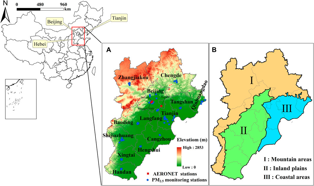
FIGURE 1. Study area with 80 monitoring stations in the Beijing–Tianjin–Hebei region (A) and sub-areas (B) divided by terrain.

PM_2.5 Monitoring Data and Predictor Variables

In addition to adding AOD to the model for [PM_2.5] prediction, it has been recognized that combining meteorological and LU information can significantly improve the model predictability (Hu et al., 2017; Wang G. et al., 2021). In this study, for the proposed two-stage statistical regression (LME + GWR) model, a main independent predictor (AOD) and eight auxiliary predictors [i.e., planetary boundary layer height (PBLH), 2-m air temperature (TEMP), 10-m wind speed (WS), relative humidity (RH, specific humidity calculated), surface pressure (PRS), precipitation (PRCP), forest coverage (FC), and urban coverage (UC)] were utilized through variables selection and multicollinearity diagnosis. The datasets covered the period from January 1, 2013, to December 31, 2020. The detail information about the datasets is shown in Table 1.

1) PM_2.5 data. The PM_2.5 hourly concentration of 80 monitoring stations in BTH was obtained from the National Urban Air Quality Real-time Release Platform. In the process of fitting the daily mean [PM_2.5], we eliminated the [PM_2.5] (i.e., <2 and >500 μg/m³) that was not within the monitoring range of the National Ambient Air Quality Standard (NAAQS) (GB 3095-2012) to ensure the validity of the PM_2.5 data.

2) AErosol RObotic NETwork (AERONET) AOD. The AOD measured by AERONET was used as the true value to verify the accuracy of the AOD retrieved by remote sensing. The AERONET AOD data (version 3, level 2) from three sites (i.e., Beijing, Beijing-CAMS, and Xianghe) were collected in our modeling area (https://aeronet.gsfc.nasa.gov/), which were used to validate the MODIS MAIAC AOD.

3) One-kilometer AOD data. High-resolution AOD products are increasingly used to capture the fine-scale differences in the spatial distribution of [PM_2.5]. The emergence of the MAIAC algorithm provided a theoretical basis for constructing a high-resolution [PM_2.5] estimation model. The MAIAC Terra/Aqua AOD (0.55 µm) products were available through the MODIS Collection-6 data record. The AERONET AOD_{550 nm} was calculated from the AOD at 675 and 440 nm using the Angstrom exponent. Simple linear regressions were carried out between the MAIAC Terra/Aqua AOD (0.55 µm) and AERONET AOD_{550 nm} at the AERONET sites for each year. The results show that the fitting with the coefficient of determination (R²) in 0.81–0.91 was acceptable in all years (Figure 2). The root mean square prediction error (RMSPE) ranged from 0.10 to 0.25, 73.15%–83.74% of the samples falling within the interval of 1 × variance, and the slope of 0.95–1.17, which met the verification accuracy requirements.

4) Meteorological data. The hourly PBLH data were derived from the Goddard Earth Observing System Model 5-Forward-processing (GEOS5-FP). Other daily meteorological data (e.g., TEMP, WS, RH, PRS, and PRCP) were extracted from the National Tibetan Plateau Data Center (TPDC) and only cover the period from 2013 to 2018 (Yang and He, 2019). The daily data from 2019 to 2020 were downloaded from the National Meteorological Science Data Center. The meteorological data in the two periods have negligible influence on the model prediction results because they have similar spatial resolutions and need to be interpolated to the same resolution as MODIS MAIAC AOD.

5) LU data. LU data were downloaded from the Geographical Information Monitoring Cloud Platform (GIM Cloud). The study selected LU data in 2015 to represent the LU status from 2013 to 2020 and extracted the urban coverage and FC in the study area into the model.

6) Data integration. Considering to match the daily [PM_2.5], the daily PBLH data were represented by averaging the observation values obtained at two times during the transit of the MODIS satellite. The daily meteorological data were then resampled to the 1-km grid by the bilinear interpolation method. In addition, the UC and FC data with 30-m spatial resolutions were averaged over the 1-km grid.

TABLE 1

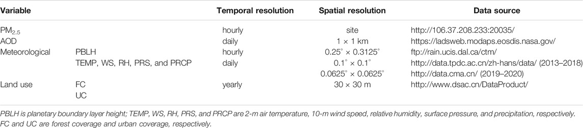
TABLE 1. Information about data source, temporal and spatial resolution.

FIGURE 2

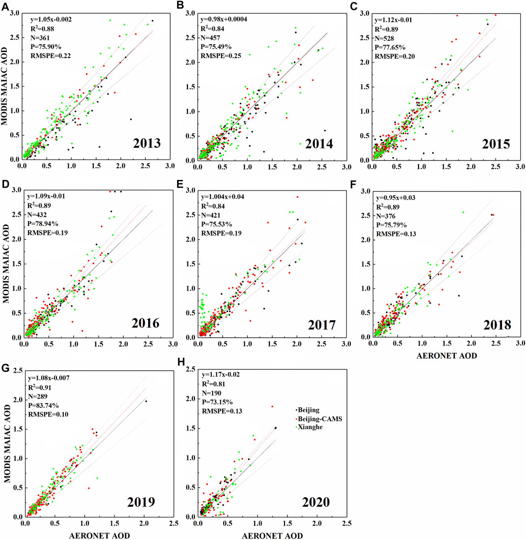
FIGURE 2. Scatter plot of MODIS MAIAC AOD and AERONET AOD at 550 nm for the period of 2013–2020 (A–H). The red dashed line is the regression line. The black line is a 1:1 line. The gray lines represent the expected error (EE) envelopes [±(0.05 + 20% × AERONET AOD)]. It also shows the coefficient of determination (R²), the number of samples (N), the percentage in EE (P), and the root mean square prediction error (RMSPE).

Methods

Collinearity Diagnosis

Considering the stability of the predictive model, the collinearity of the independent variables should be diagnosed. In this study, the variance inflation factor (VIF) and tolerance value (TV) were selected to diagnose the collinearity of the selected variables. The VIF and TV of all independent variables participating in the model satisfied VIF < 10 and TV > 0.1 for each year (Table 2), indicating that there was no collinearity problem among the independent variables and could be considered for model fitting.

TABLE 2

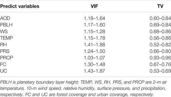
TABLE 2. The range of variance inflation factor (VIF) and tolerance value (TV) in the analysis of variable collinearity.

Two-Stage Statistics Regression Model

A two-stage statistical regression model consisting of LME model and GWR model was used to simulate the spatiotemporal variation of the PM_2.5–AOD relationship. The LME model in the first stage was applied to correct the time-varying relationship of PM_2.5–AOD. The quadratic term of AOD (AOD²) and the interaction between PBLH and AOD (PBLH × AOD) were added to the model to explain the nonlinear relationship between AOD and PM_2.5. The specific structure of the model is as follows:

$\begin{array}{l}{\text{PM}}_{2.5st}=\left({\beta }_0+{\theta }_0\right)+\left({\beta }_1+{\theta }_1\right){\text{AOD}}_{st}+\left({\beta }_2+{\theta }_2\right){\text{AOD}}_{st}^2+\left({\beta }_3+{\theta }_3\right){\text{PBLH}}_{st}+\\ \left({\beta }_4+{\theta }_4\right){\text{WS}}_{st}+\left({\beta }_5+{\theta }_5\right){\text{TEMP}}_{st}+\left({\beta }_6+{\theta }_6\right){\text{RH}}_{st}+\left({\beta }_7+{\theta }_7\right){\text{PRS}}_{st}+\left({\beta }_8+{\theta }_8\right)\\ {\text{PRCP}}_{st}+{\beta }_9\times {\text{PBLH}}_{st}\times \mathrm{AO}{\mathrm{D}}_{\mathrm{st}}+{\beta }_{10}\times \mathrm{F}{\mathrm{C}}_s+{\mathrm{\beta }}_{\mathrm{11}}\times \mathrm{U}{\mathrm{C}}_s+{\epsilon }_{st}\left({\theta }_{1\sim 8}\right)\sim N\left[\left(\mathrm{0,0,0},\psi \right)\right],{\epsilon }_{st}\sim N\left(0,{\sigma }^2\right)\end{array}(1)$

where PM_2.5st is the [PM_2.5] at station s on day t; AOD_st is the AOD of the grid cell in which the station s is positioned on day t; AOD²st is the quadratic term for AOD at station s on day t; PBLHst, WSst, TEMPst, RHst, PRSst, and PRCPst are the planetary boundary layer height, wind speed at 10-m height, temperature at 2-m height, relative humidity, surface pressure, and precipitation at station s on day t, respectively; PBLH_st × AOD_st is the interaction between PBLH and AOD at station s on day t; FC_s and UC_s are the FC value and UC value at station s, respectively; β₀ and θ₀ are the fixed and random intercepts, respectively; β₁ and β₂ are the fixed slopes of square polynomials for AOD; β₃, β₄, β₅, β₆, β₇, β₈, β₁₀, and β₁₁ are the fixed slopes of PBLH, WS, TEMP, RH, PRS, PRCP, FC, and UC; β₉ is the fixed slope of the interaction between PBLH and AOD; θ₁ and θ₂ are the daily random slopes of square polynomials for AOD; and θ₃–θ₈ are the daily random slopes of each meteorological variables, respectively.

The GWR model of the second stage was used to correct the spatial heterogeneity between PM_2.5 and AOD. The specific method was to model the residuals of the LME model. This GWR model was fitted once a day to account for temporal variability. In addition, the model using adaptive bandwidth selection methods calculated by minimizing the corrected Akaike Information Criterion (AIC) value. The specific expression is as follows:

${\text{PM}}_{2.5\_{\text{resi}}_{\text{st}}}={\beta }_0\left(u_s,v_s\right)+{\beta }_1\left(u_s,v_s\right){\text{AOD}}_{st}+{\epsilon }_{st} {\epsilon }_{st}\sim N\left(0,{\sigma }^2\right) (2)$

where PM_2.5_resi_st is the residual value from the LME model at station s in day t; AOD_st is the AOD value at station s on day t; (u_s, v_s) is the spatial coordinates of the monitoring station s; and β₀ (u_s,v_s) and β₁ (u_s,v_s) represent the regression intercept and regression slope at station s, respectively.

For model verification, a 10-fold cross-validation (CV) method was conducted to detect the degree of overfitting of the model. The entire model-fitting dataset was randomly split into 10 subsets, with each subset containing approximately 10% of the dataset. In each CV time, we selected one subset as the testing sample and used the remaining nine subsets to fit the model for prediction on the testing sample. This process was repeated 10 times to ensure that all the subsets were predicted. We fitted a linear regression was performed between the measured and predicted [PM_2.5], and the fitted R², slope, RMSPE, and relative prediction error (RPE) were evaluated the performance of the model. They represented by Eqs. 3 and 4, respectively.

$RMSPE=\sqrt{\frac{{{\displaystyle \sum }}_{i=1}^n{\left(y_{mod,i}-y_{obs,i}\right)}^2}{n} }(3)$

$RPE=\frac{RMSPE\times 100\%}{\overline{y}} (4)$

where y_mod,i is the estimated PM_2.5 at site i; y_obs,i is the observed PM_2.5 at site i; n is the total number of data samples; and $\overline{y}$ is the average of the observed PM_2.5.

The estimation process of the daily [PM_2.5] by the LME + GWR model is shown in Supplementary Figure S1.

Results

Descriptive Statistics

As shown in Table 3, the daily minimum and maximum [PM_2.5] in the BTH were ranged from 2 to 3 μg/m³ and from 371 to 499 μg/m³, respectively, which indicated that the pollution degree of different areas in the BTH had considerable differences. The annual average [PM_2.5] during the investigated period from 2013 to 2020 in the BTH were 91.27, 85.93, 72.89, 68.22, 61.02, 53.53, 45.75, and 40.97 μg/m³, respectively, indicating that the PM_2.5 pollution has been on a downward trend in the past 8 years. However, it still exceeded the limit (35 μg/m³) of the national secondary standard for ambient air quality (GB3095-2012). The average annual AOD ranged from 0.37 to 0.69 during the same period. The great difference between the mean FC and UC reflected that most of the monitoring sites in the study area were located inside or around the city. In addition, the ranges of the meteorological variables from 2013 to 2020 are also shown in Table 3.

TABLE 3

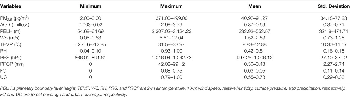
TABLE 3. Statistical indicators of modeling variables.

During the period from 2013 to 2020, the monthly [PM_2.5] monitored in the BTH demonstrated that the median monthly [PM_2.5] presented a U-shaped oscillation for each year (Figure 3). Overall, the [PM_2.5] displayed significant monthly differences, following the change pattern of “high in winter, low in summer, falling in spring and rising in autumn”. In detail, [PM_2.5] displayed a downward trend from January to May, a general stability from June to September, and an upward trend from October to December. The reason for the highest monthly [PM_2.5] in December and January was the combined effect of coal-fired heating in winter and unfavorable meteorological conditions in the BTH, such as low air humidity and weak wind speed.

FIGURE 3

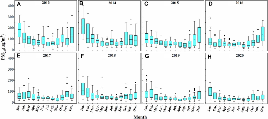
FIGURE 3. The monthly mean observed PM_2.5 concentrations from 2013 to 2020 (A–H) in the Beijing–Tianjin–Hebei region.

Model-Fitting and Validation

The comparison of LME + GWR model fitting (Figure 4A) and 10-fold CV results (Figure 4B) from 2013 to 2020 indicated that the model displayed excellent performance in capturing daily [PM_2.5]. For model fitting, the data distribution was concentrated toward the regression line. The R² ranged from 0.89 to 0.97, indicating that the two-stage model could effectively explain 89%–97% of the ground-level [PM_2.5] variation. The slope ranged from 0.89 to 1.04, indicating that only a small prediction bias remained in the model. In addition, the fitting results also displayed that the RMSPE and RPE were 6.85–24.60 μg/m³ and 16.67%–26.94%, respectively. Compared with model fitting, the 10-fold CV results showed that the CV-R², CV-RMSPE, and CV-RPE ranged from 0.85 to 0.95, 7.87 μg/m³ to 29.90 μg/m³, and 19.19–32.72%, respectively. The CV-R² decreased, and CV-RMSPE and CV-RPE increased, indicating that the model had a slight overfitting. In addition, Figure 4 shows that, when the measured [PM_2.5] exceeds 400 μg/m³, the model had a slight “high value underestimation” phenomenon.

FIGURE 4

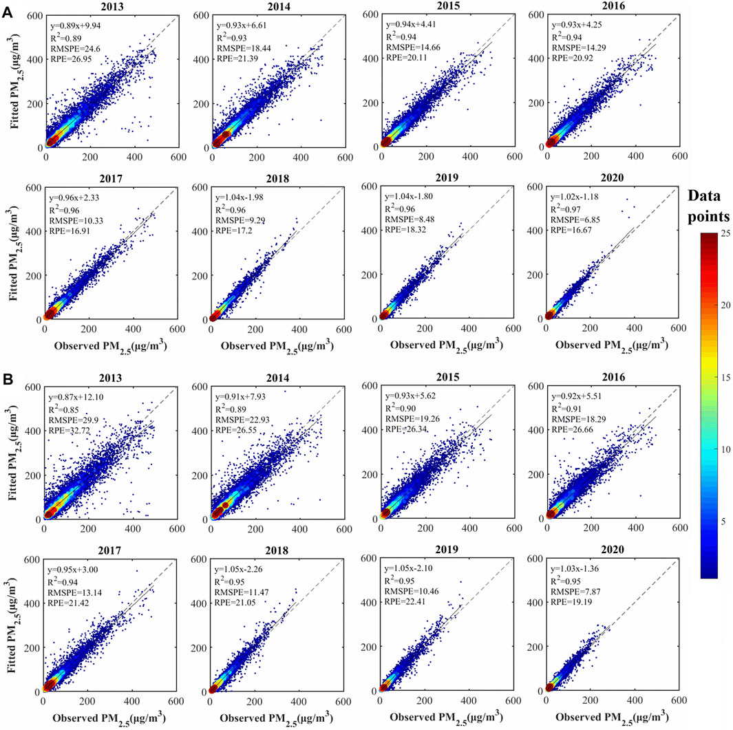
FIGURE 4. Comparison of model fitting (A) and 10-fold cross-validation (B) results from 2013 to 2020.

During the study period, the model performed best in 2020. Under the regression of the observed and predicted [PM_2.5] in the study area, CV-R² was the highest at 0.95, and the CV-RMSPE and CV-RPE were the lowest at 7.87 μg/m³ and 19.19%, respectively. This is mainly attributable to the government’s series of “Air Pollution Prevention and Control Action Plans” (APPCAP), and the [PM_2.5] has been declining year by year. About 93.72% of [PM_2.5] data samples in 2020 were less than 100 μg/m³. In contrast, the model performed the worst in 2013, with the lowest CV-R² and the largest forecast uncertainty. The main reason was that more than 32.38% of the data samples were more than 100 μg/m³, and relatively discrete data samples increased the difficulty of model fitting. Overall, the LME + GWR model that we have established was robust. Using the LME + GWR model combined with the 1-km MAIAC AOD product could excellently predict the daily near-surface [PM_2.5] with CV-R² > 0.84, CV-RMSPE < 30 μg/m³, and CV-RPE < 33% in the BTH.

Spatiotemporal Patterns of PM_2.5 Concentrations

Annual Variations

Figure 5 illustrated the annual mean [PM_2.5] estimated by the LME + GWR model, and ground-level observed [PM_2.5] from 2013 to 2020 in the BTH. The spatial variation pattern of [PM_2.5] estimated by the model was in good agreement with ground observations. The low-value areas of [PM_2.5] were located in the western and northern mountainous areas (Zone I), and the high-value areas were located in the middle and south of the BTH inland plain (Zone II). In general, the [PM_2.5] present a spatial distribution pattern of “low in the northern mountains and high in the southern plains”. During the study period, the annual mean [PM_2.5] were 69.67, 65.31, 49.26, 51.17, 44.96, 43.11, 34.54, and 32.02 μg/m³, respectively, and the overall PM_2.5 pollution level dropped significantly. Moreover, high-concentration areas ([PM_2.5] > 75 μg/m³) have shrunk remarkably, and polluted cities were mainly concentrated in Handan, Xingtai, Shijiazhuang, and Baoding.

FIGURE 5

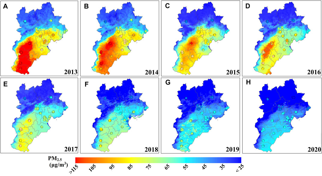
FIGURE 5. The distribution of the annual mean estimated PM_2.5 concentrations and observed PM_2.5 concentrations in the Beijing–Tianjin–Hebei region during 2013–2020 (A–H).

We adopted linear regression method to analyze the trends of annual mean [PM_2.5] in BTH. Figure 6 illustrates the spatial distribution of the slope and significance level of [PM_2.5] from 2013 to 2020. Most of the mountain areas (Zone I) in the BTH failed the significance test (p ≥ 0.01). The reason was speculated that the [PM_2.5] changed slightly during the study period. In addition, the [PM_2.5] level showed a significant decreasing trend (p < 0.05) in inland and coastal areas (Zone II and Zone III).

FIGURE 6

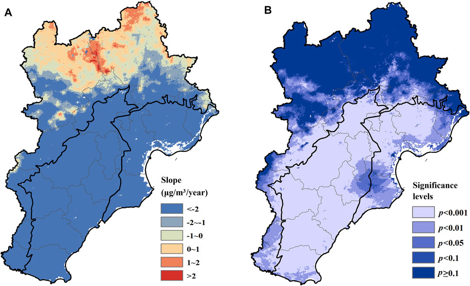
FIGURE 6. Spatial distributions of the slope (A) and significance levels (B) of annual mean PM_2.5 concentrations in the Beijing–Tianjin–Hebei region from 2013 to 2020.

Seasonal Variations

PM_2.5 pollution in the BTH displayed strong seasonal variability. On the whole, the [PM_2.5] presented the seasonal variation characteristics of “high concentration in winter, low concentration in summer, and transition between spring and autumn” (Figure 7). During the study period in winter, the mean [PM_2.5] were 117.46, 84.24, 75.30, 72.72, 55.97, 52.75, 51.48, and 51.42 μg/m³, respectively. There was a sharp decline in pollution from 2015 to 2017 and a steady decline after 2017. Compared with the [PM_2.5] in the winter of 2013, there was a decrease of 61 μg/m³ (52%) in 2017 and 66 μg/m³ (56%) in 2020. In addition, the annual and seasonal mean [PM_2.5] in the Zone II dropped the fastest compared with Zone I and Zone III (Figure 8).

FIGURE 7

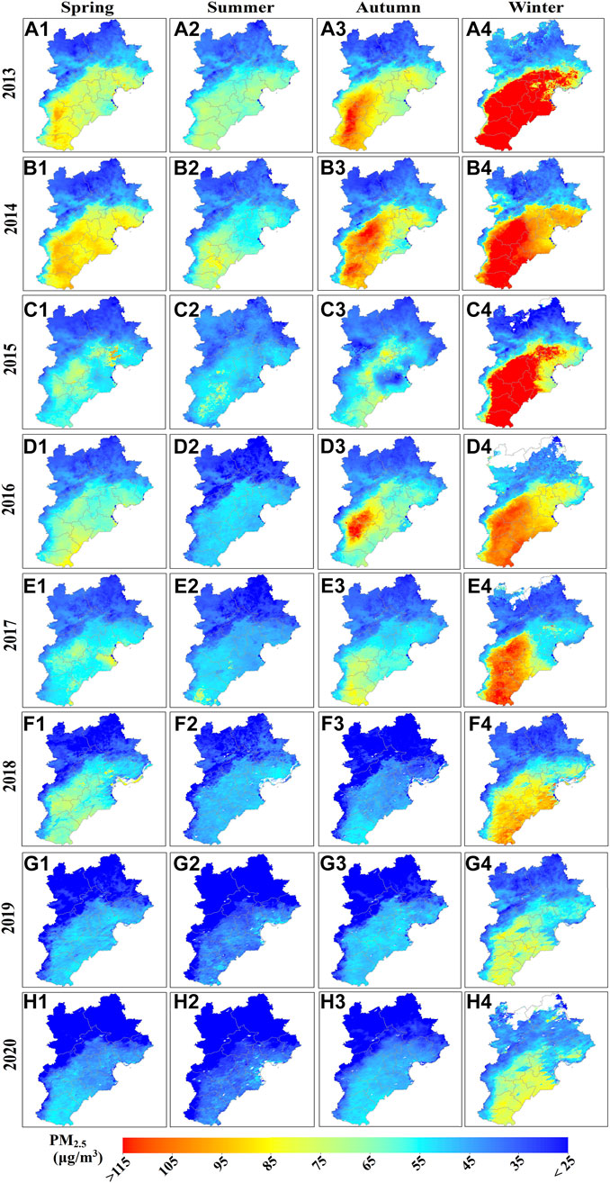
FIGURE 7. Distribution of mean PM_2.5 concentrations in spring (A1–H1), summer (A2–H2), autumn (A3–H3), and winter (A4–H4) in the Beijing–Tianjin–Hebei region during 2013–2020.

FIGURE 8

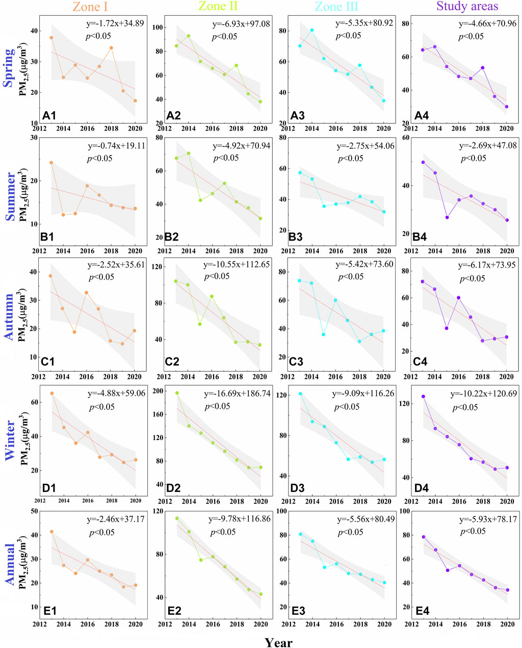
FIGURE 8. Scatter plots of seasonal and annual trends of PM_2.5 concentrations in the Zone I (A1–E1), Zone II (A2–E2), Zone III (A3–E3), and the Beijing–Tianjin–Hebei region (A4–E4) from 2013 to 2020. (The gray band represents the 95% confidence interval).

Monthly Variations

During the study period, the estimated monthly [PM_2.5] of each year presented a U-shaped pattern (Figure 9), which was consistent with the monthly measured [PM_2.5] distribution (Figure 3). January and December were the two months with the highest monthly mean [PM_2.5], which were related to coal-fired heating in the BTH. In addition, the low atmospheric humidity and temperature in these two months were also an important reason.

FIGURE 9

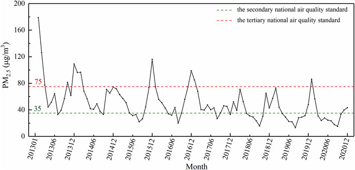
FIGURE 9. Statistical variations of the monthly mean PM_2.5 concentrations in the Beijing–Tianjin–Hebei region from 2013 to 2020.

For the spatial distribution, the mean monthly [PM_2.5] had significant differences (Figure 10). The [PM_2.5] from May to September remained at a relatively low level. From October to February of the next year, cities in inland plain areas (e.g., Shijiazhuang, Baoding, Handan, and Xingtai) had the high-level [PM_2.5].

FIGURE 10

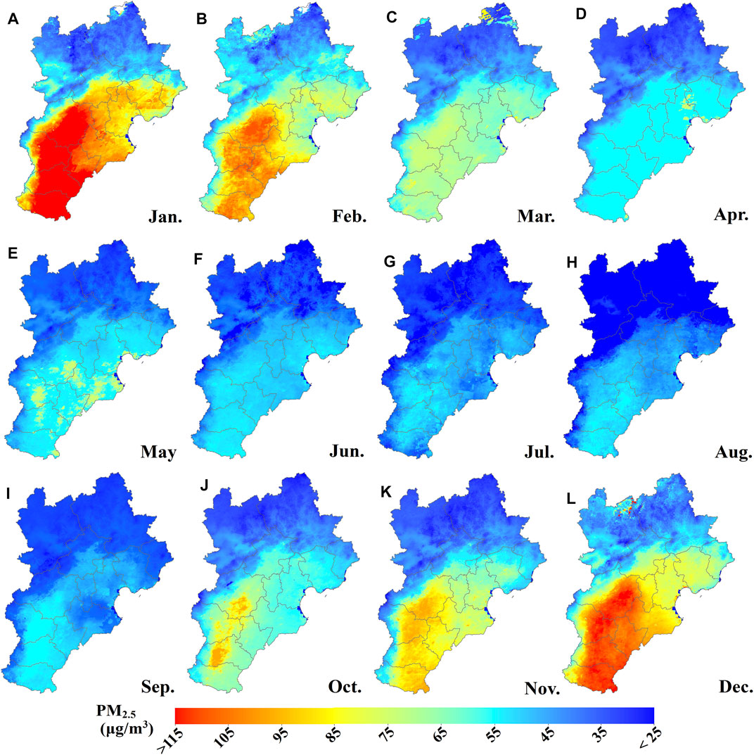
FIGURE 10. Spatial distributions of monthly mean PM_2.5 concentrations (A–L) in the Beijing–Tianjin–Hebei region during 2013–2020.

Figure 11 represents the daily fluctuations of [PM_2.5] based on station measurements and model estimates in Beijing and Shijiazhuang. The [PM_2.5] estimated by LME + GWR from 2013 to 2020 had excellent consistency with the monitoring station data and merely appeared a “high value underestimated” prediction deviation at few high concentrations (more than 400 μg/m³). The fluctuation pattern of PM_2.5 pollution in Shijiazhuang was identical with Beijing. The peak values of [PM_2.5] were mainly distributed in winter, and the peak value in Shijiazhuang (the highest of 492.28 μg/m³ appeared in 2014) was higher than that in Beijing (the highest of 463.52 μg/m³ appeared in 2015). During the study period, the annual mean [PM_2.5] in Beijing were 57.54, 54.34, 54.30, 54.53, 54.38, 39.07, 30.87, and 30.09 μg/m³, which were lower than 108.40, 91.61, 69.31, 74.48, 67.63, 53.63, 43.52, and 39.87 μg/m³ in Shijiazhuang. However, PM_2.5 fell sharply in Shijiazhuang, with a drop of 63.21% from 2013 to 2020. In addition, the frequency of high pollution in Shijiazhuang in winter was higher than that in Beijing.

FIGURE 11

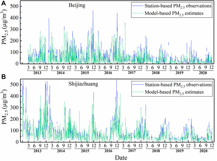
FIGURE 11. Daily fluctuation in PM_2.5 concentrations based on station observations and model-based estimates in Beijing (A) and Shijiazhuang (B).

Discussion

Causes Affecting the Spatiotemporal Distributions of PM_2.5

During the period from 2013 to 2020, [PM_2.5] in the BTH showed obvious spatiotemporal variations on different scales of annual, seasonal, and monthly. Overall [PM_2.5] in the BTH revealed a downward trend during the investigated period. Exploring the reasons for the decrease in the [PM_2.5] was inseparable from the national policy control, such as coal-to-gas and energy-saving transformation (Pan et al., 2021). In detail, the APPCAP implemented between 2013 and 2017 has successfully reduced [PM_2.5] (Yue et al., 2020), and the sharp decline in 2017 was closely related to the termination year of the APPCAP in 2017. Moreover, the [PM_2.5] in December 2015 and December 2016 were significantly higher than that in other years. The reason was that El Niño in 2015 enhanced the winter air pollution in northern China (Chang et al., 2016). The high concentration in the winter of 2016 might be influenced by anthropogenic factors (Ding et al., 2021). In addition, the [PM_2.5] in the winter of 2018–2020 decreased slowly compared with 2017, and the light-pollution areas (such as Langfang and Tangshan) slightly expanded. Furthermore, combined with the contribution of the suspension of work and production during new coronavirus disease (COVID-19) (Xian et al., 2021), the [PM_2.5] in the winter of 2020 dropped to 51.42 μg/m³, which was the lowest [PM_2.5] in winter during the study period.

In the BTH, [PM_2.5] presented the significant seasonal variation characteristics of “high in winter, low in summer, and transition between spring and autumn”, which were consistent with previous studies (Wu et al., 2016; Guo et al., 2021; Lu et al., 2021). The high [PM_2.5] in winter was concentrated in cities such as Shijiazhuang, Xingtai, and Handan. In the study areas, pollutant emissions were mainly due to the coal-fired heating and unfavorable meteorological conditions (Lv et al., 2017). Relevant studies have pointed out that the increase of boundary layer height and higher water vapor content in summer are the main reasons for the low [PM_2.5] (Qu et al., 2016; Ding et al., 2021). Moreover, the elevated [PM_2.5] levels in autumn were likely caused by the large scale straw burning in the rural areas and coal burning for heating in November (Duan et al., 2004; Lv et al., 2017). In addition, the spatiotemporal variation trends on the monthly scale follow the characteristics of seasonal changes, with the most polluted months appearing in December and January.

Comparisons With Other Studies in the Beijing–Tianjin–Hebei Region

In previous studies, the CV-R² value range of the satellite-based ground [PM_2.5] estimation model for the BTH was 0.54–0.95 (Table 4). Among these, the [PM_2.5] estimation model based on MODIS MAIAC AOD (CV-R² up to 0.82–0.95) has been found to perform better than other [PM_2.5] estimation models (a maximum CV-R² of 0.83), owing to its superior spatial resolution. Under the same high spatial resolution of AOD, our model showed similar or even better performance than other machine learning models. The performance statistics of the LME + GWR model developed was also comparable with other studies conducted in the United States that used the MODIS MAIAC AOD data (CV-R² up to 0.62–0.84) (Hu et al., 2014a, 2014b; Chudnovsky et al., 2014; Stowell et al., 2020). For model, the LME model cannot estimate the daily value of PM_2.5 at non-monitoring points, even if there are abundant data available. Models such as TEFR and STLME also have this shortcoming (Wu et al., 2016; Wang W. et al., 2021). In addition, machine learning methods that account for complex nonlinear relationships between different variables by adding hidden nodes and layers exhibited good performance in estimating [PM_2.5] (Ni et al., 2018; Stafoggia et al., 2019; Sun et al., 2019; Zhao et al., 2020; Ding et al., 2021). However, the addition of more hidden nodes and layers consumed a lot of time in estimating PM_2.5 load and produced different results for each training (Wang W. et al., 2021). Therefore, the LME + GWR model has certain advantages in terms of performance and stability. For AOD product, AHI AOD was commonly used to estimate hourly [PM_2.5] due to its high resolution. However, AHI cannot retrieve AOD at nighttime, and the quality is slightly inferior to MODIS AOD (Sun et al., 2019; Wang W. et al., 2021).

TABLE 4

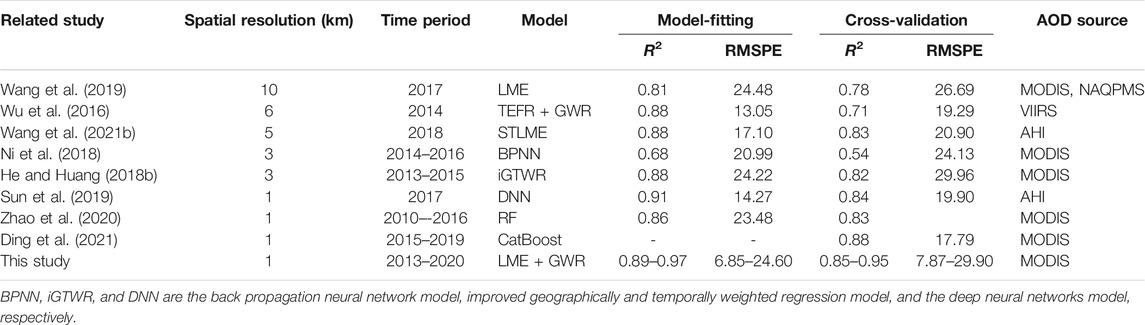
TABLE 4. Performances of previous studies on PM_2.5 estimates in the Beijing–Tianjin–Hebei region.

The model proposed in this study has many advantages. First, the high spatiotemporal resolution MAIAC Terra/Aqua fusion AOD data were employed in the model and achieved satisfactory performance. Second, the AOD quadratic term (AOD²) and the interaction term of AOD and PBLH (PBLH×AOD) were introduced into the first-stage LME model to describe the nonlinear effect of the model. Third, we adopted the GWR model as the second-stage model to improve the spatial difference of the PM_2.5–AOD. The bisquare kernel bandwidth function and adaptive bandwidth method were selected owing to the difference between the daily sample data. After CV, the degree of overfitting was very small (compared with R², CV-R² was only reduced by 0.01–0.04).

However, the model still has some limitations. One limitation was the mismatch in spatial resolution between MODIS MAIAC AOD (0.01° × 0.01°) and meteorological parameters (0.1° × 0.1° and 0.0625° × 0.0625°). Although the bilinear interpolation method for meteorological factors has proved to have better performance than linear interpolation and nearest neighbor interpolation algorithms (Zhao et al., 2020), more meteorological products with high spatial resolution were still needed. Another limitation was that we only keep three data records in some days to bring into the model. Related studies have pointed out that the overfitting degree of the two-stage model incorporating GWR decreases with the increase in the number of matching data records per day (Hu et al., 2014a; Wu et al., 2016). Therefore, too few observations in some days would lead to the GWR model to overfitting. We will explore the optimal threshold that matches the minimum number of data records later. In addition, some studies have indicated that PM_2.5 monitoring stations mostly located in cities and suburbs, and the PM_2.5 estimation in mountainous and rural areas was relatively poor (Zeng et al., 2020; Ding et al., 2021). Our study area is in the BTH with characteristics of urban industrial conditions. In particular, Hebei Province that has many rural administrative units also has a large number of factories. Provincial monitoring sites with a larger coverage area should be added to future research to increase the regional representation of the sample.

Conclusion

In this study, the two-stage model (LME + GWR) that applied MODIS MAIAC AOD and measured [PM_2.5] and meteorological and LU data as input variables was constructed to estimate the daily [PM_2.5] from 2013 to 2020 in the BTH. The LME + GWR model presented satisfactory performance (CV-R² was 0.85–0.95, RMSPE was 7.87–29.90 μg/m³, and RPE was 19.19–32.71%) and provided a well-documented dataset for air pollution monitoring. During the investigated period from 2013 to 2020, PM_2.5 pollution in the BTH region has generally been on a downward trend. This decline is mainly due to anthropogenic factors such as pollution-preventing policies, but natural factors such as climate phenomenon (El Niño) also have a certain effect. In particular, in winter season, the [PM_2.5] exhibited relatively small fluctuations from 2013 to 2014, a sharp decline occurred from 2015 to 2017, and a steady decline from 2018 to 2020.

Data Availability Statement

The original contributions presented in the study are included in the article/Supplementary Material, further inquiries can be directed to the corresponding authors.

Author Contributions

DX and WW had the idea for the article and critically revised the work; XY performed the data processing and analysis; HB and JT gave many suggestions for this paper; XY, DX, and WW prepared the manuscript. All authors read and approved the final manuscript.

Funding

This work was supported by the National Natural Science Foundation of China (no.41471091) and the High-level Talents Training and Subsidy Project of Hebei Academy of Science (202201).

Conflict of Interest

The authors declare that the research was conducted in the absence of any commercial or financial relationships that could be construed as a potential conflict of interest.

Publisher’s Note

All claims expressed in this article are solely those of the authors and do not necessarily represent those of their affiliated organizations or those of the publisher, the editors, and the reviewers. Any product that may be evaluated in this article, or claim that may be made by its manufacturer, is not guaranteed or endorsed by the publisher.

Supplementary Material

The Supplementary Material for this article can be found online at: https://www.frontiersin.org/articles/10.3389/fenvs.2022.842237/full#supplementary-material

References

Bai, Y., Wu, L., Qin, K., Zhang, Y., Shen, Y., and Zhou, Y. (2016). A Geographically and Temporally Weighted Regression Model for Ground-Level PM2.5 Estimation from Satellite-Derived 500 M Resolution AOD. Remote Sensing 8 (3), 262. doi:10.3390/rs8030262

CrossRef Full Text | Google Scholar

Chang, L., Xu, J., Tie, X., and Wu, J. (2016). Impact of the 2015 El Nino Event on Winter Air Quality in China. Sci. Rep. 6, 34275. doi:10.1038/srep34275

PubMed Abstract | CrossRef Full Text | Google Scholar

Chen, B., You, S., Ye, Y., Fu, Y., Ye, Z., Deng, J., et al. (2021). An Interpretable Self-Adaptive Deep Neural Network for Estimating Daily Spatially-Continuous PM2.5 Concentrations across China. Sci. Total Environ. 768, 144724. doi:10.1016/j.scitotenv.2020.144724

PubMed Abstract | CrossRef Full Text | Google Scholar

China, M. E. P. (2012). Ambient Air Quality Standards. GB 3095-2012. Beijing: China Environmental Science Press.

Google Scholar

Choi, M., Lim, H., Kim, J., Lee, S., Eck, T. F., Holben, B. N., et al. (2019). Validation, Comparison, and Integration of GOCI, AHI, MODIS, MISR, and VIIRS Aerosol Optical Depth over East Asia during the 2016 KORUS-AQ Campaign. Atmos. Meas. Tech. 12 (8), 4619–4641. doi:10.5194/amt-12-4619-2019

CrossRef Full Text | Google Scholar

Chow, J. C., Watson, J. G., Mauderly, J. L., Costa, D. L., Wyzga, R. E., Vedal, S., et al. (20062006). Health Effects of Fine Particulate Air Pollution: Lines that Connect. J. Air Waste Manage. Assoc. 56 (10), 1368–1380. doi:10.1080/10473289.2006.10464545

CrossRef Full Text | Google Scholar

Chudnovsky, A. A., Koutrakis, P., Kloog, I., Melly, S., Nordio, F., Lyapustin, A., et al. (2014). Fine Particulate Matter Predictions Using High Resolution Aerosol Optical Depth (AOD) Retrievals. Atmos. Environ. 89, 189–198. doi:10.1016/j.atmosenv.2014.02.019

CrossRef Full Text | Google Scholar

Ding, Y., Chen, Z., Lu, W., and Wang, X. (2021). A CatBoost Approach with Wavelet Decomposition to Improve Satellite-Derived High-Resolution PM2.5 Estimates in Beijing-Tianjin-Hebei. Atmos. Environ. 249, 118212. doi:10.1016/j.atmosenv.2021.118212

CrossRef Full Text | Google Scholar

Duan, F., Liu, X., Yu, T., and Cachier, H. (2004). Identification and Estimate of Biomass Burning Contribution to the Urban Aerosol Organic Carbon Concentrations in Beijing. Atmos. Environ. 38, 1275–1282. doi:10.1016/j.atmosenv.2003.11.037

CrossRef Full Text | Google Scholar

Engel-cox, J. A., Holloman, C. H., Coutant, B. W., and Hoff, R. M. (2004). Qualitative and Quantitative Evaluation of MODIS Satellite Sensor Data for Regional and Urban Scale Air Quality. Atmos. Environ. 38 (16), 2495–2509. doi:10.1016/j.atmosenv.2004.01.039

CrossRef Full Text | Google Scholar

Engel-Cox, J., Kim Oanh, N. T., van Donkelaar, A., Martin, R. V., and Zell, E. (2013). Toward the Next Generation of Air Quality Monitoring: Particulate Matter. Atmos. Environ. 80, 584–590. doi:10.1016/j.atmosenv.2013.08.016

CrossRef Full Text | Google Scholar

Gu, Y., Wong, T. W., Law, C. K., Dong, G. H., Ho, K. F., Yang, Y., et al. (2018). Impacts of Sectoral Emissions in China and the Implications: Air Quality, Public Health, Crop Production, and Economic Costs. Environ. Res. Lett. 13 (8), 084008. doi:10.1088/1748-9326/aad138

CrossRef Full Text | Google Scholar

Guo, W., Zhang, B., Wei, Q., Guo, Y., Yin, X., Li, F., et al. (2021). Estimating Ground-Level PM2.5 Concentrations Using Two-Stage Model in Beijing-Tianjin-Hebei, China. Atmos. Pollut. Res. 12 (9), 101154. doi:10.1016/j.apr.2021.101154

CrossRef Full Text | Google Scholar

Gupta, P., and Christopher, S. A. (2009). Particulate Matter Air Quality Assessment Using Integrated Surface, Satellite, and Meteorological Products: Multiple Regression Approach. J. Geophys. Res. 114, D14205. doi:10.1029/2008JD011496

CrossRef Full Text | Google Scholar

He, Q., Gu, Y., and Zhang, M. (2020). Spatiotemporal Trends of PM2.5 Concentrations in central China from 2003 to 2018 Based on MAIAC-Derived High-Resolution Data. Environ. Int. 137, 105536. doi:10.1016/j.envint.2020.105536

PubMed Abstract | CrossRef Full Text | Google Scholar

He, Q., and Huang, B. (2018b). Satellite-based High-Resolution PM2.5 Estimation over the Beijing-Tianjin-Hebei Region of China Using an Improved Geographically and Temporally Weighted Regression Model. Environ. Pollut. 236, 1027–1037. doi:10.1016/j.envpol.2018.01.053

PubMed Abstract | CrossRef Full Text | Google Scholar

He, Q., and Huang, B. (2018a). Satellite-based Mapping of Daily High-Resolution Ground PM2.5 in China via Space-Time Regression Modeling. Remote Sensing Environ. 206, 72–83. doi:10.1016/j.rse.2017.12.018

CrossRef Full Text | Google Scholar

Hu, X., Belle, J. H., Meng, X., Wildani, A., Waller, L. A., Strickland, M. J., et al. (2017). Estimating PM2.5 Concentrations in the Conterminous United States Using the Random Forest Approach. Environ. Sci. Technol. 51 (12), 6936–6944. doi:10.1021/acs.est.7b01210

PubMed Abstract | CrossRef Full Text | Google Scholar

Hu, X., Waller, L. A., Al-Hamdan, M. Z., Crosson, W. L., Estes, M. G., Estes, S. M., et al. (2013). Estimating Ground-Level PM2.5 Concentrations in the southeastern U.S. Using Geographically Weighted Regression. Environ. Res. 121, 1–10. doi:10.1016/j.envres.2012.11.003

PubMed Abstract | CrossRef Full Text | Google Scholar

Hu, X., Waller, L. A., Lyapustin, A., Wang, Y., Al-Hamdan, M. Z., Crosson, W. L., et al. (2014a). Estimating Ground-Level PM2.5 Concentrations in the Southeastern United States Using MAIAC AOD Retrievals and a Two-Stage Model. Remote Sensing Environ. 140, 220–232. doi:10.1016/j.rse.2013.08.032

CrossRef Full Text | Google Scholar

Hu, X., Waller, L. A., Lyapustin, A., Wang, Y., and Liu, Y. (2014b). 10-year Spatial and Temporal Trends of PM2.5 Concentrations in the southeastern US Estimated Using High-Resolution Satellite Data. Atmos. Chem. Phys. 14 (12), 6301–6314. doi:10.5194/acp-14-6301-2014

PubMed Abstract | CrossRef Full Text | Google Scholar

Kahn, R., Banerjee, P., Mcdonald, D., and Diner, D. J. (1998). Sensitivity of Multiangle Imaging to Aerosol Optical Depth and to Pure-Particle Size Distribution and Composition over Ocean. J. Geophys. Res. 103 (D24), 32195–32213. doi:10.1029/98JD01752

CrossRef Full Text | Google Scholar

Lee, H. J., Liu, Y., Coull, B. A., Schwartz, J., and Koutrakis, P. (2011). A Novel Calibration Approach of MODIS AOD Data to Predict PM2.5 Concentrations. Atmos. Chem. Phys. 11 (15), 7991–8002. doi:10.5194/acp-11-7991-2011

CrossRef Full Text | Google Scholar

Li, T., Shen, H., Zeng, C., Yuan, Q., and Zhang, L. (2017). Point-surface Fusion of Station Measurements and Satellite Observations for Mapping PM2.5 Distribution in China: Methods and Assessment. Atmos. Environ. 152, 477–489. doi:10.1016/j.atmosenv.2017.01.004

CrossRef Full Text | Google Scholar

Liang, F., Xiao, Q., Wang, Y., Lyapustin, A., Li, G., Gu, D., et al. (2018). MAIAC-based Long-Term Spatiotemporal Trends of PM2.5 in Beijing, China. Sci. Total Environ. 616-617, 1589–1598. doi:10.1016/j.scitotenv.2017.10.155

PubMed Abstract | CrossRef Full Text | Google Scholar

Liu, Y., Paciorek, C. J., and Koutrakis, P. (2009). Estimating Regional Spatial and Temporal Variability of PM 2.5 Concentrations Using Satellite Data, Meteorology, and Land Use Information. Environ. Health Perspect. 117 (6), 886–892. doi:10.1289/ehp.0800123

PubMed Abstract | CrossRef Full Text | Google Scholar

Liu, Y., Park, R. J., Jacob, D. J., Li, Q., Kilaru, V., and Sarnat, J. A. (2004). Mapping Annual Mean Ground-Level PM2.5concentrations Using Multiangle Imaging Spectroradiometer Aerosol Optical Thickness over the Contiguous United States. J. Geophys. Res. 109, a–n. doi:10.1029/2004jd005025

CrossRef Full Text | Google Scholar

Lu, J., Zhang, Y., Chen, M., Wang, L., Zhao, S., Pu, X., et al. (2021). Estimation of Monthly 1 Km Resolution PM2.5 Concentrations Using a Random forest Model over "2 + 26" Cities, China. Urban Clim. 35, 100734. doi:10.1016/j.uclim.2020.100734

CrossRef Full Text | Google Scholar

Lv, B., Hu, Y., Chang, H. H., Russell, A. G., Cai, J., Xu, B., et al. (2017). Daily Estimation of Ground-Level PM2.5 Concentrations at 4 Km Resolution over Beijing-Tianjin-Hebei by Fusing MODIS AOD and Ground Observations. Sci. Total Environ. 580, 235–244. doi:10.1016/j.scitotenv.2016.12.049

PubMed Abstract | CrossRef Full Text | Google Scholar

Lyapustin, A., Wang, Y., Korkin, S., and Huang, D. (2018). MODIS Collection 6 MAIAC Algorithm. Atmos. Meas. Tech. 11 (10), 5741–5765. doi:10.5194/amt-11-5741-2018

CrossRef Full Text | Google Scholar

Ma, Z., Hu, X., Sayer, A. M., Levy, R., Zhang, Q., Xue, Y., et al. (2016). Satellite-Based Spatiotemporal Trends in PM 2.5 Concentrations: China, 2004-2013. Environ. Health Perspect. 124 (2), 184–192. doi:10.1289/ehp.1409481

PubMed Abstract | CrossRef Full Text | Google Scholar

Moazami, S., Noori, R., Amiri, B. J., Yeganeh, B., Partani, S., and Safavi, S. (2016). Reliable Prediction of Carbon Monoxide Using Developed Support Vector Machine. Atmos. Pollut. Res. 7 (3), 412–418. doi:10.1016/j.apr.2015.10.022

CrossRef Full Text | Google Scholar

Ni, X., Cao, C., Zhou, Y., Cui, X., and P. Singh, R. (2018). Spatio-Temporal Pattern Estimation of PM2.5 in Beijing-Tianjin-Hebei Region Based on MODIS AOD and Meteorological Data Using the Back Propagation Neural Network. Atmosphere 9, 105. doi:10.3390/atmos9030105

CrossRef Full Text | Google Scholar

Pan, X., Zhao, Y., and Wang, M. (2021). Impact of COVID-19 on Extremely Polluted Air Quality and Trend Forecast in Seven Provinces and Three Cities of China. Front. Environ. Sci. 9, 770900. doi:10.3389/fenvs.2021.770900

CrossRef Full Text | Google Scholar

Polezer, G., Tadano, Y. S., Siqueira, H. V., Godoi, A. F. L., Yamamoto, C. I., de André, P. A., et al. (2018). Assessing the Impact of PM2.5 on Respiratory Disease Using Artificial Neural Networks. Environ. Pollut. 235, 394–403. doi:10.1016/j.envpol.2017.12.111

PubMed Abstract | CrossRef Full Text | Google Scholar

Qu, W., Wang, J., Zhang, X., Sheng, L., and Wang, W. (2016). Opposite Seasonality of the Aerosol Optical Depth and the Surface Particulate Matter Concentration over the North China Plain. Atmos. Environ. 127, 90–99. doi:10.1016/j.atmosenv.2015.11.061

CrossRef Full Text | Google Scholar

Riediker, M., Franc, Y., Bochud, M., Meier, R., and Rousson, V. (2018). Exposure to Fine Particulate Matter Leads to Rapid Heart Rate Variability Changes. Front. Environ. Sci. 6, 2. doi:10.3389/fenvs.2018.00002

CrossRef Full Text | Google Scholar

Schaap, M., Apituley, A., Timmermans, R. M. A., Koelemeijer, R. B. A., and de Leeuw, G. (2009). Exploring the Relation between Aerosol Optical Depth and PM2.5 at Cabauw, the Netherlands. Atmos. Chem. Phys. 9, 909–925. doi:10.5194/acp-9-909-2009

CrossRef Full Text | Google Scholar

Stafoggia, M., Bellander, T., Bucci, S., Davoli, M., de Hoogh, K., de' Donato, F., et al. (2019). Estimation of Daily PM10 and PM2.5 Concentrations in Italy, 2013-2015, Using a Spatiotemporal Land-Use Random-forest Model. Environ. Int. 124, 170–179. doi:10.1016/j.envint.2019.01.016

PubMed Abstract | CrossRef Full Text | Google Scholar

Stowell, J. D., Bi, J., Al-Hamdan, M. Z., Lee, H. J., Lee, S.-M., Freedman, F., et al. (2020). Estimating PM2.5 in Southern California Using Satellite Data: Factors that Affect Model Performance. Environ. Res. Lett. 15 (9), 094004. doi:10.1088/1748-9326/ab9334

CrossRef Full Text | Google Scholar

Sun, Y., Zeng, Q., Geng, B., Lin, X., Sude, B., and Chen, L. (2019). Deep Learning Architecture for Estimating Hourly Ground-Level PM2.5 Using Satellite Remote Sensing. IEEE Geosci. Remote Sensing Lett. 16 (9), 1343–1347. doi:10.1109/lgrs.2019.2900270

CrossRef Full Text | Google Scholar

van Donkelaar, A., Martin, R. V., and Park, R. J. (2006). Estimating Ground-Level PM2.5using Aerosol Optical Depth Determined from Satellite Remote Sensing. J. Geophys. Res. 111, D21201. doi:10.1029/2005JD006996

CrossRef Full Text | Google Scholar

Wang, G., Leng, W., Jiang, S., and Cao, B. (2021a). Long-Term Variation in Wintertime Atmospheric Diffusion Conditions over the Sichuan Basin. Front. Environ. Sci. 9, 763504. doi:10.3389/fenvs.2021.763504

CrossRef Full Text | Google Scholar

Wang, J., and Christopher, S. A. (2003). Intercomparison between Satellite-Derived Aerosol Optical Thickness and PM2.5mass: Implications for Air Quality Studies. Geophys. Res. Lett. 30 (21), 2095. doi:10.1029/2003gl018174

CrossRef Full Text | Google Scholar

Wang, Q., Zeng, Q., Tao, J., Sun, L., Zhang, L., Gu, T., et al. (2019). Estimating PM2.5 Concentrations Based on MODIS AOD and NAQPMS Data over Beijing-Tianjin-Hebei. Sensors 19 (5), 1207. doi:10.3390/s19051207

PubMed Abstract | CrossRef Full Text | Google Scholar

Wang, W., He, J., Miao, Z., and Du, L. (2021b). Space-Time Linear Mixed-Effects (STLME) Model for Mapping Hourly fine Particulate Loadings in the Beijing-Tianjin-Hebei Region, China. J. Clean. Prod. 292, 125993. doi:10.1016/j.jclepro.2021.125993

CrossRef Full Text | Google Scholar

Wang, X., Sun, W., Zheng, K., Ren, X., and Han, P. (2020). Estimating Hourly PM2.5 Concentrations Using MODIS 3 Km AOD and an Improved Spatiotemporal Model over Beijing-Tianjin-Hebei, China. Atmos. Environ. 222, 117089. doi:10.1016/j.atmosenv.2019.117089

CrossRef Full Text | Google Scholar

Wu, J., Yao, F., Li, W., and Si, M. (2016). VIIRS-based Remote Sensing Estimation of Ground-Level PM2.5 Concentrations in Beijing-Tianjin-Hebei: A Spatiotemporal Statistical Model. Remote Sensing Environ. 184, 316–328. doi:10.1016/j.rse.2016.07.015

CrossRef Full Text | Google Scholar

Xian, T., Li, Z., and Wei, J. (2021). Changes in Air Pollution Following the COVID-19 Epidemic in Northern China: The Role of Meteorology. Front. Environ. Sci. 9, 654651. doi:10.3389/fenvs.2021.654651

CrossRef Full Text | Google Scholar

Xiao, Q., Wang, Y., Chang, H. H., Meng, X., Geng, G., Lyapustin, A., et al. (2017). Full-coverage High-Resolution Daily PM2.5 Estimation Using MAIAC AOD in the Yangtze River Delta of China. Remote Sensing Environ. 199, 437–446. doi:10.1016/j.rse.2017.07.023

CrossRef Full Text | Google Scholar

Xue, W., Zhang, J., Zhong, C., Ji, D., and Huang, W. (2020). Satellite-derived Spatiotemporal PM2.5 Concentrations and Variations from 2006 to 2017 in China. Sci. Total Environ. 712, 134577. doi:10.1016/j.scitotenv.2019.134577

PubMed Abstract | CrossRef Full Text | Google Scholar

Yan, J.-W., Tao, F., Zhang, S.-Q., Lin, S., and Zhou, T. (2021). Spatiotemporal Distribution Characteristics and Driving Forces of PM2.5 in Three Urban Agglomerations of the Yangtze River Economic Belt. Ijerph 18, 2222. doi:10.3390/ijerph18052222

PubMed Abstract | CrossRef Full Text | Google Scholar

Yang, K., and He, J. (2019). China Meteorological Forcing Dataset (1979-2018). National Tibetan Plateau Data Center. doi:10.11888/AtmosphericPhysics.tpe.249369.file

CrossRef Full Text | Google Scholar

Yang, W., He, Z., Huang, H., and Huang, J. (2021). A Clustering Framework to Reveal the Structural Effect Mechanisms of Natural and Social Factors on PM2.5 Concentrations in China. Sustainability 13 (3), 1428. doi:10.3390/su13031428

CrossRef Full Text | Google Scholar

Yao, F., Si, M., Li, W., and Wu, J. (2018). A Multidimensional Comparison between MODIS and VIIRS AOD in Estimating Ground-Level PM2.5 Concentrations over a Heavily Polluted Region in China. Sci. Total Environ. 618, 819–828. doi:10.1016/j.scitotenv.2017.08.209

PubMed Abstract | CrossRef Full Text | Google Scholar

Yao, F., Wu, J., Li, W., and Peng, J. (2019). A Spatially Structured Adaptive Two-Stage Model for Retrieving Ground-Level PM2.5 Concentrations from VIIRS AOD in China. ISPRS J. Photogrammetry Remote Sensing 151, 263–276. doi:10.1016/j.isprsjprs.2019.03.011

CrossRef Full Text | Google Scholar

Yeganeh, B., Hewson, M. G., Clifford, S., Knibbs, L. D., and Morawska, L. (2017). A Satellite-Based Model for Estimating PM2.5 Concentration in a Sparsely Populated Environment Using Soft Computing Techniques. Environ. Model. Softw. 88, 84–92. doi:10.1016/j.envsoft.2016.11.017

CrossRef Full Text | Google Scholar

Yue, H., He, C., Huang, Q., Yin, D., and Bryan, B. A. (2020). Stronger Policy Required to Substantially Reduce Deaths from PM2.5 Pollution in China. Nat. Commun. 11, 1462. doi:10.1038/s41467-020-15319-4

PubMed Abstract | CrossRef Full Text | Google Scholar

Zeng, Q., Tao, J., Chen, L., Zhu, H., Zhu, S., and Wang, Y. (2020). Estimating Ground-Level Particulate Matter in Five Regions of China Using Aerosol Optical Depth. Remote Sensing 12, 881. doi:10.3390/rs12050881

CrossRef Full Text | Google Scholar

Zhang, K., de Leeuw, G., Yang, Z., Chen, X., Su, X., and Jiao, J. (2019b). Estimating Spatio-Temporal Variations of PM2.5 Concentrations Using VIIRS-Derived AOD in the Guanzhong Basin, China. Remote Sensing 11 (22), 2679. doi:10.3390/rs11222679

CrossRef Full Text | Google Scholar

Zhang, R., Di, B., Luo, Y., Deng, X., Grieneisen, M. L., Wang, Z., et al. (2018). A Nonparametric Approach to Filling Gaps in Satellite-Retrieved Aerosol Optical Depth for Estimating Ambient PM2.5 Levels. Environ. Pollut. 243 (Pt B), 998–1007. doi:10.1016/j.envpol.2018.09.052

PubMed Abstract | CrossRef Full Text | Google Scholar

Zhang, Z., Wu, W., Fan, M., Wei, J., Tan, Y., and Wang, Q. (2019a). Evaluation of MAIAC Aerosol Retrievals over China. Atmos. Environ. 202, 8–16. doi:10.1016/j.atmosenv.2019.01.013

CrossRef Full Text | Google Scholar

Zhao, B., Wang, S., Ding, D., Wu, W., Chang, X., Wang, J., et al. (2019). Nonlinear Relationships between Air Pollutant Emissions and PM2.5-related Health Impacts in the Beijing-Tianjin-Hebei Region. Sci. Total Environ. 661, 375–385. doi:10.1016/j.scitotenv.2019.01.169

PubMed Abstract | CrossRef Full Text | Google Scholar

Zhao, C., Wang, Q., Ban, J., Liu, Z., Zhang, Y., Ma, R., et al. (2020). Estimating the Daily PM2.5 Concentration in the Beijing-Tianjin-Hebei Region Using a Random forest Model with a 0.01° × 0.01° Spatial Resolution. Environ. Int. 134, 105297. doi:10.1016/j.envint.2019.105297

PubMed Abstract | CrossRef Full Text | Google Scholar