Capturing Spatial Influence in Wind Prediction With a Graph Convolutional Neural Network

Nowadays, wind power is playing a significant role in power systems; it is necessary to improve the prediction accuracy, which will help make better use of wind sources. The existing neural network methods, such as recurrent neural network (RNN), have been widely used in wind prediction; however, RNN models only consider the dynamic change of temporal conditions and ignore the spatial correlation. In this work, we combine the graph convolutional neural (GCN) with the gated recurrent unit (GRU) to do prediction on simulated and real wind speed and wind power data sets. The improvements of prediction results by GCN in all wind speed experiments show its ability to capture spatial dependence and improve prediction accuracy. Although the GCN does not perform well in short-term wind power prediction as the change of wind power data is not so smooth due to the limitation of turbine operation, the results of long-term prediction still prove the performance of GCN.

Introduction

In order to deal with the crises of fuel energy and environmental pollution, wind energy is being widely developed all over the world, and wind power is starting to play a hugely significant role in power systems (Liu and Guan, 2004). However, the large amount of wind power generation also brings great challenges to the stable operation of power systems due to the variable and stochastic nature of wind (Defferrard et al., 2016). For example, wind power fluctuation caused a challenge event reported by the Electric Reliability Council of Texas (ECROT). To mitigate the harmful impacts, accurate wind prediction is always required by system operators (Zhang et al., 2016).

Wind prediction, including wind speed and wind power prediction, uses a large amount of historical wind data to train a fitting model between inputs and outputs. Wind speed is the most relevant factor in determining wind power. In particular, the wind power curves for different types of wind turbines roughly have the same shape (Pinson, 2013); hence, one approach to modeling wind power is to model the wind speed and associate it to the wind power using wind power curves suitable for a given wind farm (Stohl et al., 1995).

Wind speed can be modeled as a spatiotemporal process as it evolves randomly in time and space. However, wind forecasting has always been a challenge due to its complex spatial and temporal dependences.

Existing wind speed forecasting models can be categorized as physical, statistical, and machine learning models. Physical models use mathematical expressions to model highly complex and nonlinear dynamics of atmospheric flow to produce numerical wind predictions (Yan and Ouyang, 2019). Gneiting et al. (2006) applied a second order model that uses the spatiotemporal covariance as a basis for estimation in Irish wind prediction. This model is quite suitable when the underlying process can be modeled as a Gaussian spatiotemporal field and is one basic type of spatiotemporal process used in the modeling of wind. Statistical methods rely on relevant historical data to predict future wind generation, traditionally using models such as the history average model (HA) (Liu and Guan, 2004) or the autoregressive integrated moving average model (ARIMA). A multichannel adaptive filter is used to forecast wind speed and direction using spatial correlations at multiple sites in Dowell et al. (2014). Markov chain–based statistical methods that leverage a graphic spatiotemporal learning-based model and statistical characteristics of aggregated wind generation are presented in He et al. (2014) to forecast wind generation output. As for machine learning methods, the recurrent neural network (RNN) is the most widely used neural network model in processing time series data. The long short-term memory (LSTM) model (Hochreiter and Schmidhuber, 1997) and the gated recurrent unit (GRU) model (Cho et al., 2014) are variants of the RNN that can avoid the gradient disappearance and explosion that can occur in RNN. The basic principles of the LSTM and GRU are roughly the same; they all use a gated mechanism to memorize as much long-term information as possible and are equally effective for various tasks (Chung et al., 2014). However, due to its complex structure, LSTM has a longer training time while the GRU model has a relatively simple structure, fewer parameters, and faster training ability.

However, both LSTM and GRU models only consider the dynamic change of temporal conditions and ignore the spatial dependence given that the change of wind condition is also restricted by the surrounding environment. Intuitively, the flow of wind in nearby regions affect each other. As there exists a strong correlation between wind sites located in a vicinity, the information collected from neighboring sites will help improve the prediction accuracy of target sites (Liu et al., 2020), which can be effectively handled by the convolutional neural network (CNN), which has shown its powerful ability to get spatial structural information (LeCun et al., 1998). A CNN uses filters to find relationships between neighboring inputs, which can make it easier for the network to converge on the correct solution.

The traditional CNN can obtain local spatial features in Euclidean space, but the relation network between each wind farm is in the form of a graph that is not a two-dimensional grid, which means the CNN model cannot deal with the complex topological structure of the wind relation network. However, the graph neural network (GNN) is good at handling the arbitrary graph structure data. To model the spatial correlations in graph-structured data, a graph CNN is developed to capture the spatial dependence, and a similar approach has been used in traffic prediction and shown good performance (Zhao et al., 2019).

There has been some work that applied GNN in wind prediction such as Mei Yu’s (Yu et al., 2020) and Mahdi Khodayar’s work (Khodayar and Wang, 2018), but all these works were based on NREL data sets, which are simulation data sets and do not provide real wind speed or power data. They showed the results in a one-time experiment only, whereas the neural network model’s performance will be slightly different each time as the character of itself.

In this work, to demonstrate that the GNN model does have the ability to utilize the spatial correlations to improve accuracy in real wind prediction, we combine the graph convolutional network (GCN) with the GRU model to do prediction on five different wind data sets, including three wind speed data sets and two wind power data sets. Moreover, the GCN-GRU model is validated not only in 10 m height but also in 100 m height wind speed prediction. Furthermore, the final results are based on a collection of 10 experiments for each data set. The forecasting results show a steady state under different prediction horizons, which indicates that the GCN-GRU model can not only achieve short-term prediction, but can also be used for long-term wind prediction tasks.

Review of the Literature

Recently, given RNN’s strong ability in processing time series problems, improved LSTM and GRU models have been applied in wind prediction. Zhewen Niu proposed a novel sequence-to-sequence model using the attention-based gated recurrent unit (AGRU) that improves accuracy of forecasting processes (Niu et al., 2020). A novel data-driven approach is proposed by Adam Kisvari in wind power forecasting by integrating data preprocessing, resampling, anomaly detection and treatment, feature engineering, and hyperparameter tuning based on gated recurrent deep learning models and critically compared with the algorithm of LSTM (Kisvari et al., 2021). Ruiguo Yu proposed an improved LSTM-enhanced forget-gate network model, abbreviated as LSTM-EFG, used in forecasting wind power (Yu et al., 2019). Xiaohui Yuan’s simulation results showed that the PIWP obtained by the Beta-PSO-LSTM model has higher reliability and narrower interval bandwidth, which can provide decision support for the safe and stable operation of power systems (Yuan et al., 2019). In Yao Liu’s work, a wind power short-term forecasting method based on discrete wavelet transform and LSTM networks (DWT_LSTM) is proposed. The discrete wavelet transform is introduced to decompose the nonstationary wind power time series into several components that have more stationarity and are easier to predict (Liu et al., 2019).

There is also some work that applies GNN in wind prediction, such as Mei Yu proposing the superposition graph neural network (SGNN) for feature extraction, which can maximize the use of spatial and temporal features for prediction. In the four offshore wind farms used in experiments, the mean square error of the method is reduced by 9.80%–22.53% compared with current advanced methods, and the prediction stability of the method has also been greatly improved (Yu et al., 2020). Mahdi Khodayar proposed GCDLA to capture spatial wind features as well as deep temporal features of the wind data at each wind site. Simulation results show the advantages of capturing deep spatial and temporal interval features in the proposed framework compared with the state-of-the-art deep learning models as well as shallow architectures in the recent literature (Khodayar and Wang, 2018). However, Mei Yu’s work is about offshore wind, which is more stable than the wind on land as the surrounding terrain has a great influence on it. Mahdi Khodayar’s work used the mutual information matrix to process the graph model. Furthermore, these two studies both worked on simulation data sets, and their results were based on a one-time experiment only, so it is hard to say that the improvement of prediction results by GNN is not occasional.

Problem Definition

In this paper, the goal of wind forecasting is to predict the wind speed or power in a certain period of time based on the historical wind information of several sites in a specific area. In our experiments, the wind information can be wind speed or wind power data.

Wind Network $\mathit{G}$

As shown in Figure 1, the wind of the target site may be influenced by the wind flows from its surrounding sites, we describe these wind sites in a specific area as a wind network although this network is unseen. We use an undirected graph $G=\left(V,E\right)$ to describe the topological structure of the wind network. We treat each wind site as a node, where $V$ is a set of nodes, $V=\left\{v_1,v_2,\dots ,v_N\right\}$, $N$ is the number of the nodes, and $E$ is a set of edges between each wind site. The adjacency matrix $A$ is used to represent the connection among wind sites, $A\in R^{N\times N}$. In this work, the adjacency matrix $A$ is processed by normalization of a distance matrix, which is calculated by the distance between each wind site in the wind network. Note that distance is calculated in an “as the crow flies” sense and does not take the intervening topography into account.

FIGURE 1

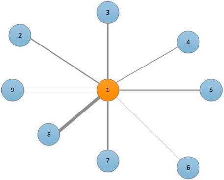
FIGURE 1. The wind speed of the central site is affected by the wind from its surrounding site; the thickness of edges indicates the strength of the correlation.

Feature Matrix ${\mathrm{X}}^{\mathrm{N\times P}}$

We regard the wind speed or power as the attribute feature of the nodes in the network, expressed as $X^{N\times P}$, where $P$ represents the number of node attribute features (the length of the historical time series) and $X_t\in R^{N\times i}$ is used to represent the speed or power on each site at time $i$. Again, the node attribute feature can be any wind information, such as wind speed, wind direction, wind, or wind power.

Model

To evaluate the GCN’s ability to capture the spatial features in wind prediction, we combine the GCN model with the GRU model and then compare the performance of the GCN-GRU model with the GRU model through several evaluation metrics. The flow chart of the GCN-GRU model is shown in Figure 2.

FIGURE 2

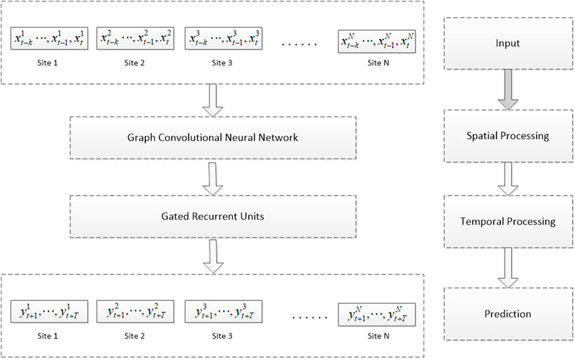
FIGURE 2. Flow chart of the GCN-GRU model.

Spatial Model

The target site is influenced by a complex wind network formed by its surrounding sites, and in this work, we use the GCN to capture spatial correlations. Existing GCNs can be divided into two main categories: spatial- and spectral-based GCNs (Liu et al., 2020). Spatial-based GCNs directly define the convolutional operation by operating on spatially close—the first or second order neighbors—such that the convolutional operation using different weight matrices for nodes with different degrees (Duvenaud et al., 2015). Considering the wind farms are all connected if we treat them in a graph domain, we choose to use the spectral-based GCN to capture the effect of surrounding wind farms.

In 2014, a spectral network was proposed in Bruna et al. (2013). It transforms the samples into Fourier domains to perform convolution operations through Fourier transform, and then the samples are transformed back to the graph domains through inverse Fourier transform. Specifically, the graph convolutional operation of the sample $X\in R^N$ can be defined as

$G\ast X=U{G}_W{U}^{T}X,(1)$

where $\ast$ is the graph convolutional operation, $U$ is the matrix of eigenvectors of the normalized graph Laplacian $L=I_N-D^{-\frac{1}{2}}A{D}^{-\frac{1}{2}}=U\wedge U^T$ with a diagonal matrix of its eigenvalues $\wedge$ and $U^{T}X$ being the graph Fourier transform of $X$, and $G_W=diag\left(U^{T}G\right)$ is the filter parameterized by $W\in R^n$.

In Defferrard et al. (2016), the Chebyshev spectral CNN (ChebNet) that approximate $G_W$ by the truncated expansion of Chebyshev polynomials $T_k\left(X\right)$ up to $K^{th}$ is proposed. To circumvent the problem of being computationally expensive, $G_W$ can be approximated by a truncated expansion in terms of Chebyshev polynomials $T_k\left(X\right)$ up to the $K^{th}$ order:

$G\ast X\approx {\displaystyle \sum }_{k=0}^K{W}_k{T}_k\left(\frac{2L}{{\lambda }_{max}}-I_n\right)X(2)$

$T_k\left(X\right)=2X{T}_{k-1}\left(X\right)-T_{k-2}\left(X\right)T_0\left(X\right)=1T_1\left(X\right)=X,$

where $W\in R^K$ is a vector that consists of Chebyshev coefficients and ${\lambda }_{max}$ is the largest eigenvalue. Because the operation is a $K^{th}$ order polynomial in the Laplacian, it is K-localized.

Moreover, if we set $K=1$ and ${\lambda }_{max}=2$, we can get a linear function on the graph Laplacian spectrum:

$G\ast X\approx W_{0}X-W_1{D}^{-\frac{1}{2}}A{D}^{-\frac{1}{2}}X.(3)$

Furthermore, to restrain the number of parameters and alleviate overfitting problems, we assume that $W=W_0=W_1$ (Berg et al., 2017) and then set $\widehat{A}=A+I_n$ to do renormalization to avoid vanishing gradients problems (Kipf and Welling, 2016), which lead to the following formula:

$G\ast X\approx W\left(I_n+D^{-\frac{1}{2}}A{D}^{-\frac{1}{2}}\right)X={\widehat{D}}^{-\frac{1}{2}}\widehat{A}{\widehat{D}}^{-\frac{1}{2}}XW(4)$

where $\widehat{D}$ denotes the diagonal matrix of node degree with $D_{ii}={\displaystyle \sum }_{j=1}^n{\widehat{a}}_{ij}$.

In summary, we use a two2-layer GCN model based on Eq. 5 to learn spatial features from wind data and it can be expressed as

$f\left(X_t,\text{Λ}\right)=\sigma \left(\text{Λ}\left(Relu\left(\text{Λ}{X}_t{W}_0\right)\right)W_1\right),(5)$

where $X_t$ represents the features matrix at time $t$, $\text{Λ}$ is the adjacency matrix calculated by the distance between each wind site, $\text{Λ}={\widehat{D}}^{-\frac{1}{2}}\widehat{A}{\widehat{D}}^{-\frac{1}{2}}$ denotes preprocessing step in Eq. 4, $\widehat{A}=A+I_N$ is a matrix with self-connection structure, and $\widehat{D}$ is a degree matrix. $W_0$ and $W_1$ represent the weight matrix in the first and second GCN layer, and $\sigma \left(\text{·}\right)$ and $Relu\left(\right)$ represent the activation function.

Temporal Model

After spatial processing by the GCN model, we get a new feature matrix $X_t^{\text{'}}$, and we can have new time series data to do time prediction. In this work, as our key goal is to evaluate the GCN’s performance in wind prediction, a simpler and faster model to do time forecasting is needed. As the GRU model has a relatively simple structure and fewer parameters than LSTM, we chose the GRU model to obtain temporal dependence from the wind data.

As shown in Figure 3, $h_{t-1}$ denotes the hidden state at time $t-1$; $X_t^{\text{'}}$ denotes the wind information at time $t$; $r_t$ is the reset gate, which is used to control the degree of ignoring the status information at the previous moment; $u_t$ is the update gate, which is used to control the degree to which the status information at the previous time is brought into the current status; $c_t$ is the memory content stored at time $t$; and $h_t$ is output state at time $t$. The GRU obtains the wind status at time $t$ by taking the hidden status at time $t-1$ and the current wind information as inputs. While capturing the wind information at the current moment, the model still retains the changing trend of historical wind information and has the ability to capture temporal dependence.

$u_t=\sigma \left(W_u\left[X_t^{\prime },h_{t-1}\right]+b_u\right)$

$r_t=\sigma \left(W_r\left[X_t^{\prime },h_{t-1}\right]+b_r\right)$

$c_t=tanh(W_c[X_t^{\prime },(r_t\ast h_{t-1})]+b_c)(6)$

$h_t=u_t\ast h_{t-1}+\left(1-u_t\right)\ast c_t$

In these equations, $X_t^{\text{'}}$ is the new wind information processed by GCN, $W$ and $b$ represent the weights and deviations in the training process.

FIGURE 3

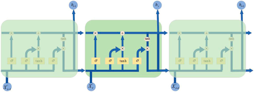
FIGURE 3. The architecture of GRU model.

Loss Function

In the training step, the goal of the GCN-GRU model is to learn the well-fitted parameters by minimizing the error between the real wind data and the predicted wind value. We use ${\mathit{Y}}_{\mathit{t}}$ and ${\widehat{Y}}_t$ to denote the real wind and the predicted speed or power data, respectively. The loss function is shown in Eq. 7. The first term is used to minimize the error between the real traffic speed and the prediction. The second term $L_{reg}$ is an L2 regularization term that helps to avoid an overfitting problem, and λ is a hyperparameter:

$loss=\left|\right|Y_t-{\widehat{Y}}_t\left|\right|+\lambda L_{reg}.(7)$

Experiments

In this section, we evaluate the prediction performance of GCN-GRU model on five data sets.

Data Description

(1) Two Canadian climate wind speed data sets. One of them includes nine stations, and the other includes 19 stations. These real wind speed data are all recorded at 10 m height, and the stations are all located in Alberta. We chose the wind speed data from the historical climate data set, which can be downloaded from the Canada Environment and natural resources website. (https://climate.weather.gc.ca/historical_data/search_historic_data_e.html).

(2) Two Eastern wind integration data sets. One includes wind speed data from 10 sites, and the other contains the corresponding wind power data at the same places. The wind speed data was downloaded from the National Renewable Energy Laboratory (NREL) website (https://www.nrel.gov/grid/wind-integration-data.html), and the corresponding wind power data set was computed by the Renewable Energy Potential (reV) Model (Maclaurin et al., 2019) by a given set of latitude and longitude coordinates. Different from the Canada climate wind speed data, the NREL wind speed data are simulated by predictive models at 100 m height.

(3) One NRGStream wind power data set. We chose seven wind farms listed by the Alberta Electric System Operator (AESO) and use the hourly wind power data from 2018 to 2019.

In the experiments, the input data was normalized to the interval [0,1]. In addition, 80% of the data was used as the training set and the remaining 20% was used as the testing set. We predicted the wind speed of the next 1, 2, and 3 h. The detailed information of these data sets can be found in Supplementary Materials.

Evaluation Metrics

To evaluate the performance of the GCN model, we use three metrics of the difference between the real wind data $Y_t$ and the prediction $\widehat{Y_t}$, including

(1) Root mean squared error (RMSE)

$RMSE=\sqrt{\frac{1}{n}{\displaystyle \sum }_{i=1}^n{(Y_t-{\widehat{Y}}_t)}^2}.$

(2) Mean absolute error

$MAE= \frac{1}{n}{\displaystyle \sum }_{i=1}^n|Y_t-{\widehat{Y}}_t|.$

(3) Accuracy

$Accuracy=1- \frac{\left|\right|Y_t-{\widehat{Y}}_t|{|}_F}{\left|\right|Y|{|}_F}.$

Parameter Settings

Our goal is to see whether the GCN can capture the environment information and improve the prediction result. As the GCN-GRU and GRU share the same GRU model, we use the same parameters for GCN-GRU and GRU, such as the amount of GRU unit, the learning rate, the training epoch, and batch size.

For the input layer, the training data set (80% of the overall data) is taken as input in the training process, and the remaining data is used as input in the testing process. The GCN-GRU model is trained using the Adam optimizer.

Experiment Results

In this part, we compare the performance of the GCN-GRU and GRU models and also show the prediction results with some other baseline methods, includin: (1) HA (Pinson, 2013), which uses the average wind information in the historical periods as the prediction; (2) ARIMA (Stohl et al., 1995), which fits the observed time series into a parametric model to predict future wind data; and (3) the support vector regression model (SVR) (Smola and Schölkopf, 2004), which uses historical data to train the model and obtains the relationship between the input and output and then predicts by giving the future wind data. We use the linear kernel, and the penalty term is 0.001.

As the GCN-GRU model is also based on GRU, according to the experiments, we find that the GRU’s prediction is not quite stable; that is, the result is a little different each time as the neural network optimization based on stochastic gradient descent to find the global minimum is different each time. To show that the prediction improvement by the GCN is not incidental, we repeat each experiment 10 times to calculate the standard error and show the range of the prediction results. As prediction accuracy of each station is different, Tables 1–3 give the result of a specific station whose prediction accuracy is best.

TABLE 1

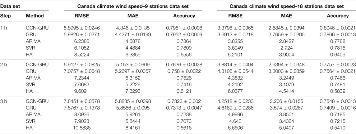
TABLE 1. The best results in Canada climate wind speed experiments.

TABLE 2

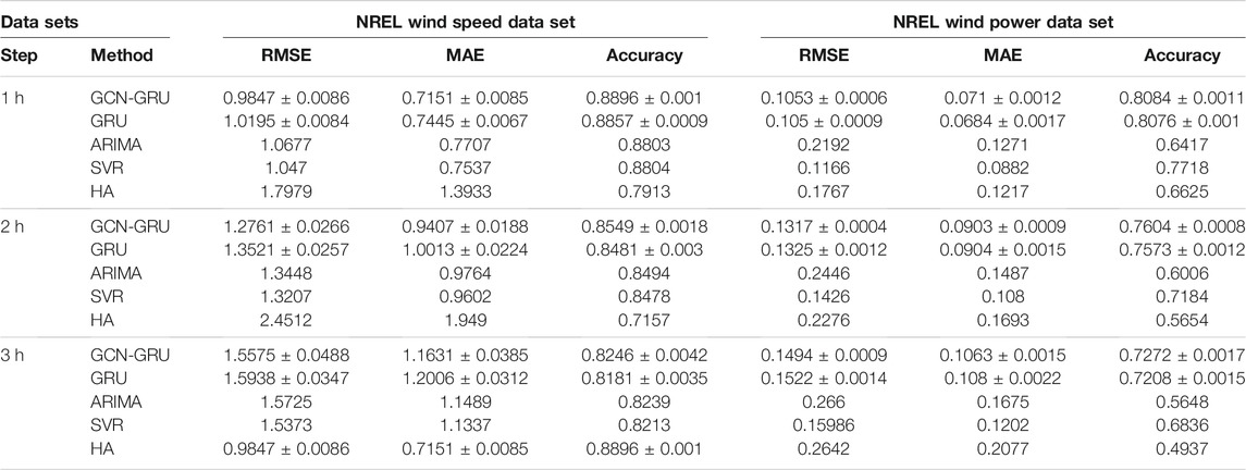
TABLE 2. The results of NREL wind experiments.

TABLE 3

TABLE 3. NRGStream wind power experiments.

We can see that the neural network models, including the GCN-GRU and GRU models, achieve better prediction precision than other baselines, such as ARIMA, SVR, and HA. For example, for the 1-h wind speed prediction on the data set of “Canada climate wind speed experiment–nine stations,” the RMSE of the GCN-GRU and the GRU models are approximately 5.4% and 4.1% lower than that of the ARIMA model, and the accuracy of these are improved by 1.4% and 1.1%. Compared with the SVR model, the RMSE of the GCN-GRU and the GRU models are reduced by 3.4% and 2.1%, and the accuracy is approximately 2.2% and 1.8% higher than that of the SVR model. The RMSE error of the GCN-GRU and GRU models are reduced by approximately 30.7% and 29.8% compared with the HA model, and the accuracies are approximately 14.2% and 13.9% higher than that of HA. Next, we focus on the comparisons between GCN-GRU’s and GRU’s results.

Tables 1, 2 show the prediction results of the GCN-GRU model, GRU model and other baseline methods for Canada climate wind speed data sets, NREL wind speed data, and NREL wind power data, respectively. By comparing the experiments of GCN-GRU and GRU in these four experiments, we can see that all the GCN-GRU results are better than the GRU model. It shows that GCN can capture some geographical information and improve the prediction performance.

In the nine-station Canada climate wind speed prediction, we can see that, comparing with GRU, there is 0.0831 improvement for RMSE evaluation and approximately 0.3% improvement in accuracy. In the nine-station Canada climate wind speed prediction, we can see that there is 0.3114 improvement for RMSE evaluation and approximately 1.8% improvement in accuracy. To explain the difference in the Canada climate nine- and 18-station experiments, although they are all wind prediction at 10 m height, we note that more wind stations can provide more surrounding information; that is why the 18 stations experiment’s result is much better than nine stations.

By comparing the experiment results of NREL wind speed with the Canada climate wind speed experiment, we can see that the accuracy is much higher for all models. It mainly because the NREL data is about the wind at 100 m height, and the change of the wind is more stable than the wind of the Canada climate at 10 m height, which makes the model easier to predict. From these four experiments, we can see that the GCN model can improve the prediction accuracy.

However, we find that the prediction accuracy of all these models gets lower in NREL wind power prediction when we compare with NREL wind speed prediction. What is more, the GCN-GRU model almost achieves same prediction accuracy with the GRU model in 1-h step prediction. The reason for these unsatisfactory results mainly is that the NREL data sets are simulated by mathematic models other than real recorded data. Thus, we do another experiment based on the NRGStream data set, which records the real wind power from wind farms in Alberta, Canada.

According to the NRGStream wind power experiment, we can find that the GCN-GRU model has even worse performance in 1 h prediction. In the simulated and real wind power experiments, we can see that the GCN does not perform as well as in wind speed prediction. It is mainly because the wind power data is not so smooth as the wind speed data due to the operation intervention of wind farms, such as when the wind speed is higher than the limitation of the turbines; the wind power data will always be the highest value other than keeping increasing when the wind speed increases. If the wind speed is less than the specific speed that the turbines need, the wind power data is zero directly other than a small value like the wind speed. What is more, some wind farms may directly shut down wind turbines to protect them when the wind is extremely strong while others nearby may keep running. The character of wind power data leads to the lower prediction accuracy.

What is more, for the sake of showing the improvement of prediction results by GCN is not occasional, we also calculate the average value of prediction results of all wind stations in wind speed and power forecasting experiments. From Tables 4–6, we can see that GCN not only improves the prediction result for a specific station, it also owns the ability to enhance prediction accuracy for all wind stations although it still has a drawback when predict the wind power directly.

TABLE 4

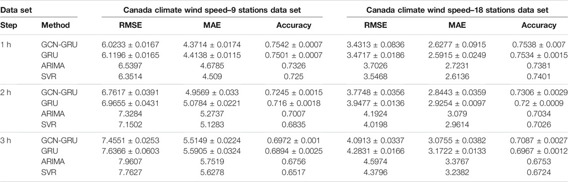
TABLE 4. The average value of prediction results of all wind stations in Canada Climate wind speed experiments.

TABLE 5

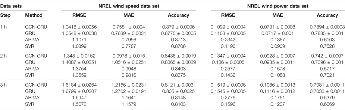
TABLE 5. The average value of prediction results of all wind stations in NREL wind experiments

TABLE 6

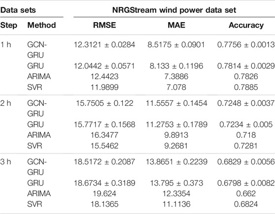
TABLE 6. The average value of prediction results of all wind stations in NRGStream wind power experiments.

Comparison of the Prediction Between GCN-GRU and GRU

Figures 4, 5 are the prediction comparisons between GCN-GRU and GRU in wind speed and wind power prediction. In Figure 4, we can see that the change of wind speed is smooth although the curve fluctuates strongly. However, the interventions of wind turbines are obvious in both the NREL and NRGStream wind power, there exist many horizontal lines in the wind power data, and these interventions may lead to the bad performance of GCN in wind power predictions.

FIGURE 4

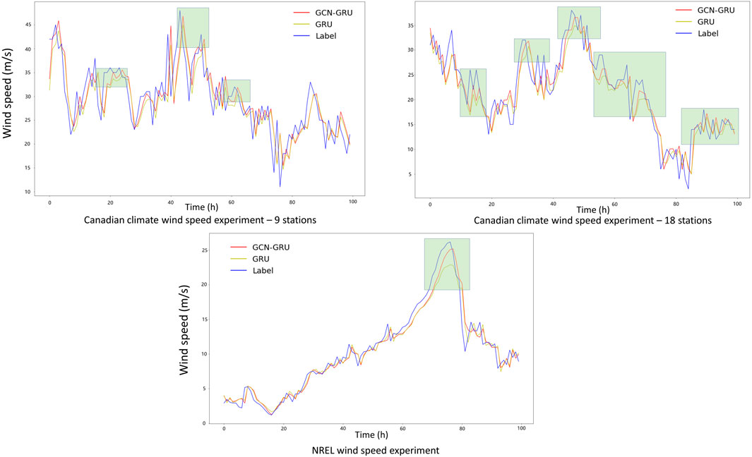
FIGURE 4. Comparison of three wind speed prediction experiments between GCN-GRU and GRU; the light green areas are where GCN-GRU’s prediction curves closer to the real curve, namely, GCN-GRU performs better than GRU in one-step wind speed prediction.

FIGURE 5

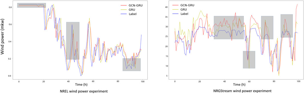
FIGURE 5. Comparison of two wind power prediction experiments between GCN-GRU and GRU; the gray areas are where GRU’s prediction curves closer to real curve, namely, GRU performs better than GCN-GRU in one-step wind power prediction.

Conclusion

In this paper, a GCN model is proposed to improve precision of wind prediction; we evaluate the GCN-GRU model not only on 10 and 100 m height wind speed prediction, but also through wind power prediction. To show the performance of the GCN-GRU model, the final results are based on a collection of 10 experiments for each data set; the forecasting results are quite stable in different prediction steps. Although the GCN-GRU model does not achieve better performance than the GRU model in short-term NRGStream wind power prediction, the results of five different wind data sets prove GCN’s ability to capture spatial influence and improve the prediction results. Finally, our study offers new findings and may add considerable value to the energy management field; our finding confirms that the GCN model has positive influence on wind prediction. What is more, the failure of GCN in short-term wind power prediction also tells us that, if we want to achieve a higher accuracy in wind power prediction, it is better to combine the wind speed prediction with the wind power data.

Data Availability Statement

The original contributions presented in the study are included in the article/Supplementary Material, further inquiries can be directed to the corresponding author.

Author Contributions

Conceived and designed the experiments: ZL TW Analyzed the data: ZL Wrote the paper: ZL TW.

Funding

ZL is supported by the CSC Scholarship offered by the China Scholarship Council.

Conflict of Interest

The authors declare that the research was conducted in the absence of any commercial or financial relationships that could be construed as a potential conflict of interest.

Publisher’s Note

All claims expressed in this article are solely those of the authors and do not necessarily represent those of their affiliated organizations, or those of the publisher, the editors and the reviewers. Any product that may be evaluated in this article, or claim that may be made by its manufacturer, is not guaranteed or endorsed by the publisher.

Supplementary Material

The Supplementary Material for this article can be found online at: https://www.frontiersin.org/articles/10.3389/fenvs.2022.836050/full#supplementary-material

References

Ahmadian, A., Sedghi, M., Aliakbar-Golkar, M., Fowler, M., and Elkamel, A. (2016). Two-layer Optimization Methodology for Wind Distributed Generation Planning Considering Plug-In Electric Vehicles Uncertainty: A Flexible Active-Reactive Power Approach. Energ. Convers. Management 124, 231–246. doi:10.1016/j.enconman.2016.07.025

CrossRef Full Text | Google Scholar

Ahmed, M. S., and Cook, A. R. (1979). Analysis of Freeway Traffic Time-Series Data by Using Box-Jenkins Techniques. No. 722. Washington: Transportation Research Board.

Google Scholar

Berg, R. V. D., Kipf, T. N., and Welling, M. (2017). Graph Convolutional Matrix Completion. arXiv [Preprint]. Available at: https://arxiv.org/abs/1706.02263.

Google Scholar

Bruna, J., Zaremba, W., Szlam, A., and LeCun, Y. (2013). Spectral Networks and Locally Connected Networks on Graphs. arXiv [Preprint]. Available at: https://arxiv.org/abs/1312.6203.

Google Scholar

Cho, K., Van Merriënboer, B., Bahdanau, D., and Bengio, Y. (2014). On the Properties of Neural Machine Translation: Encoder-Decoder Approaches. arXiv [Preprint]. Available at: https://arxiv.org/abs/1409.1259.

Google Scholar

Choi, S.-D., Baek, S.-Y., Chang, Y.-S., Wania, F., Ikonomou, M. G., Yoon, Y.-J., et al. (2008). Passive Air Sampling of Polychlorinated Biphenyls and Organochlorine Pesticides at the Korean Arctic and Antarctic Research Stations: Implications for Long-Range Transport and Local Pollution. Environ. Sci. Technol. 42 (19), 7125–7131. doi:10.1021/es801004p

PubMed Abstract | CrossRef Full Text | Google Scholar

Chung, J., Gulcehre, C., Cho, K., and Bengio, Y. (2014). Empirical Evaluation of Gated Recurrent Neural Networks on Sequence Modeling. arXiv [Preprint]. Available at: https://arxiv.org/abs/1412.3555.

Google Scholar

Defferrard, M., Bresson, X., and Vandergheynst, P. (2016). Convolutional Neural Networks on Graphs with Fast Localized Spectral Filtering. Adv. Neural Inf. Process. Syst. 29, 3844–3852.

Google Scholar

Dowell, J., Weiss, S., Hill, D., and Infield, D. (2014). Short-term Spatio-Temporal Prediction of Wind Speed and Direction. Wind Energy 17 (12), 1945–1955. doi:10.1002/we.1682

CrossRef Full Text | Google Scholar

Duvenaud, D., Maclaurin, D., Aguilera-Iparraguirre, J., Gómez-Bombarelli, R., Hirzel, T., Aspuru-Guzik, A., et al. (2015). Convolutional Networks on Graphs for Learning Molecular Fingerprints, Advances in neural information processing systems.

Google Scholar

Gneiting, T., Genton, M., and Guttorp, P. (2006). Geostatistical Space-Time Models, Stationarity, Separability, and Full Symmetry. Monogr. Stat. Appl. Probab. 107, 151–175. doi:10.1201/9781420011050.ch4

CrossRef Full Text | Google Scholar

He, M., Yang, L., Zhang, J., and Vittal, V. (2014). A Spatio-Temporal Analysis Approach for Short-Term Forecast of Wind Farm Generation. IEEE Trans. Power Syst. 29 (4), 1611–1622. doi:10.1109/tpwrs.2014.2299767

CrossRef Full Text | Google Scholar

Hochreiter, S., and Schmidhuber, J. (1997). Long Short-Term Memory. Neural Comput. 9 (8), 1735–1780. doi:10.1162/neco.1997.9.8.1735

PubMed Abstract | CrossRef Full Text | Google Scholar

Hong, K. R., Qiu, L. S., Yang, D. X., and Jiang, M. (2021). Spatio-Temporal Evolution and Correlation Analysis of Urban Land Use Patterns and Air Quality in Pearl River Delta, China. Front. Environ. Sci. 472. doi:10.3389/fenvs.2021.698383

CrossRef Full Text | Google Scholar

Khodayar, M., and Wang, J. (2018). Spatio-temporal Graph Deep Neural Network for Short-Term Wind Speed Forecasting. IEEE Trans. Sustainable Energ. 10 (2), 670–681. doi:10.1109/TSTE.2018.2844102

CrossRef Full Text | Google Scholar

Kipf, T. N., and Welling, M. (2016). Semi-supervised Classification with Graph Convolutional Networks. arXiv [Preprint]. Available at: https://arxiv.org/abs/1609.02907.

Google Scholar

Kisvari, A., Lin, Z., and Liu, X. (2021). Wind Power Forecasting - A Data-Driven Method along with Gated Recurrent Neural Network. Renew. Energ. 163, 1895–1909. doi:10.1016/j.renene.2020.10.119

CrossRef Full Text | Google Scholar

LeCun, Y., Bottou, L., Bengio, Y., and Haffner, P. (1998). Gradient-based Learning Applied to Document Recognition. Proc. IEEE 86 (11), 2278–2324. doi:10.1109/5.726791

CrossRef Full Text | Google Scholar

Liu, J., and Guan, W. (2004). A Summary of Traffic Flow Forecasting Methods [J]. J. Highw. transportation Res. Dev. 3, 82–85.

Google Scholar

Liu, Y., Guan, L., Hou, C., Han, H., Liu, Z., Sun, Y., et al. (2019). Wind Power Short-Term Prediction Based on LSTM and Discrete Wavelet Transform. Appl. Sci. 9 (6), 1108. doi:10.3390/app9061108

CrossRef Full Text | Google Scholar

Liu, Y., Liu, Y., and Yang, C. (2020). Modulation Recognition with Graph Convolutional Network. IEEE Wireless Commun. Lett. 9 (5), 624–627. doi:10.1109/lwc.2019.2963828

CrossRef Full Text | Google Scholar

Maclaurin, G. J., Grue, N. W., Lopez, A. J., and Heimiller, D. M. (2019). The Renewable Energy Potential (Rev) Model: A Geospatial Platform for Technical Potential and Supply Curve Modeling. No. NREL/TP-6A20-73067. Golden, CO (United States): National Renewable Energy Lab.(NREL.

Google Scholar

Mu, L., Su, J., Mo, X., Peng, N., Xu, Y., Wang, M., et al. (2021). The Temporal-Spatial Variations and Potential Causes of Dust Events in Xinjiang Basin During 1960–2015. Front. Environ. Sci. 360. doi:10.3389/fenvs.2021.727844

CrossRef Full Text | Google Scholar

Niu, Z., Yu, Z., Tang, W., Wu, Q., and Reformat, M. (2020). Wind Power Forecasting Using Attention-Based Gated Recurrent Unit Network. Energy 196, 117081. doi:10.1016/j.energy.2020.117081

CrossRef Full Text | Google Scholar

Paramati, S. R., Shahzad, U., and Doğan, B. (2022). The Role of Environmental Technology for Energy Demand and Energy Efficiency: Evidence from OECD Countries. Renew. Sustainable Energ. Rev. 153, 111735. doi:10.1016/j.rser.2021.111735

CrossRef Full Text | Google Scholar

Pinson, P. (2013). Wind Energy: Forecasting Challenges for its Operational Management. Stat. Sci. 28 (4), 564–585. doi:10.1214/13-sts445

CrossRef Full Text | Google Scholar

Shahzad, U., Schneider, N., and Ben Jebli, M. (2021). How Coal and Geothermal Energies Interact with Industrial Development and Carbon Emissions? An Autoregressive Distributed Lags Approach to the Philippines. Resour. Pol. 74, 102342. doi:10.1016/j.resourpol.2021.102342

CrossRef Full Text | Google Scholar

Skogland, T. (1984). Wild Reindeer Foraging-Niche Organization. Ecography 7 (4), 345–379. doi:10.1111/j.1600-0587.1984.tb01138.x

CrossRef Full Text | Google Scholar

Smola, A. J., and Schölkopf, B. (2004). A Tutorial on Support Vector Regression. Stat. Comput. 14 (3), 199–222. doi:10.1023/b:stco.0000035301.49549.88

CrossRef Full Text | Google Scholar

Stohl, A., Wotawa, G., Seibert, P., and Kromp-Kolb, H. (1995). Interpolation Errors in Wind fields as a Function of Spatial and Temporal Resolution and Their Impact on Different Types of kinematic Trajectories. J. Appl. Meteorol. 34 (10), 2149–2165. doi:10.1175/1520-0450(1995)034<2149:ieiwfa>2.0.co;2

CrossRef Full Text | Google Scholar

Wizelius, T. (2015). Developing Wind Power Projects: Theory and Practice. London: Routledge.

Google Scholar

Yan, J., and Ouyang, T. (2019). Advanced Wind Power Prediction Based on Data-Driven Error Correction. Energ. Convers. Manag. 180, 302–311. doi:10.1016/j.enconman.2018.10.108

CrossRef Full Text | Google Scholar

Yu, M., Zhang, Z., Li, X., Yu, J., Gao, J., Liu, Z., et al. (2020). Superposition Graph Neural Network for Offshore Wind Power Prediction. Future Generation Computer Syst. 113, 145–157. doi:10.1016/j.future.2020.06.024

CrossRef Full Text | Google Scholar

Yu, R., Gao, J., Yu, M., Lu, W., Xu, T., Zhao, M., et al. (2019). LSTM-EFG for Wind Power Forecasting Based on Sequential Correlation Features. Future Generation Computer Syst. 93, 33–42. doi:10.1016/j.future.2018.09.054

CrossRef Full Text | Google Scholar

Yuan, X., Chen, C., Jiang, M., and Yuan, Y. (2019). Prediction Interval of Wind Power Using Parameter Optimized Beta Distribution Based LSTM Model. Appl. Soft Comput. 82, 105550. doi:10.1016/j.asoc.2019.105550

CrossRef Full Text | Google Scholar

Zha, X., Ouyang, T., Qin, L., Xiong, Y., and Huang, H. (2016). Selection of Time Window for Wind Power Ramp Prediction Based on Risk Model. Energ. Convers. Management 126, 748–758. doi:10.1016/j.enconman.2016.08.064

CrossRef Full Text | Google Scholar

Zhang, Z., Zhang, X., Gong, D., Kim, S.-J., Mao, R., and Zhao, X. (2016). Possible Influence of Atmospheric Circulations on winter Haze Pollution in the Beijing-Tianjin-Hebei Region, Northern China. Atmos. Chem. Phys. 16 (2), 561–571. doi:10.5194/acp-16-561-2016

CrossRef Full Text | Google Scholar

Zhao, L., Song, Y., Zhang, C., Liu, Y., Wang, P., Lin, T., et al. (2019). T-gcn: A Temporal Graph Convolutional Network for Traffic Prediction. IEEE Trans. Intell. Transportation Syst. 21 (9), 3848–3858.

Google Scholar