 Lajiao Chen
 Zhidan Hu4
 Mohd Yawar Ali Khan
 Jie Wen
95% of researchers rate our articles as excellent or good
Learn more about the work of our research integrity team to safeguard the quality of each article we publish.
Find out more
ORIGINAL RESEARCH article
Front. Environ. Sci. , 21 February 2022
Sec. Environmental Informatics and Remote Sensing
Volume 10 - 2022 | https://doi.org/10.3389/fenvs.2022.798336
This article is part of the Research Topic Big Earth Data Intelligence for Environmental Modeling View all 15 articles
Optimality principles have been applied in ecohydrological modeling to derive optimal vegetation properties and describe co-evolution states of vegetation and water cycle. Unfortunately, most existing optimality-based models only consider vertical vegetation-soil-water interactions on plot scale, without considering the lateral hydrological processes. This work aims to extend the field-scale Vegetation Optimality Model (VOM) to the watershed scale. Lateral flow is incorporated to VOM through a hierarchical strategy, establishing the Distributed Vegetation Optimality Model (DisVOM). The model is tested with long-tem flux measurements in the Walnut Gulch watershed, a United States Agricultural Research Service (US-ARS) experimental watershed in southern Arizona. The results indicate the model performance is acceptable for most of years, especially for the growing season. The seasonal dynamic of ET, soil water, and GPP demonstrate good consistency with observations. The model provides reasonable spatial distribution of ET and GPP, suggesting the model can discriminate the effect of lateral flow on water redistribution, and consequently on root water uptake, as well as carbon assimilation. The model could be a useful tool assessing the impact of climate change and human activities on vegetation and water cycle.
Vegetation and the water cycle are intrinsically coupled through physical and biological processes, such as carbon, water, energy, and nutrients exchange (Rodriguez-Iturbe et al., 1999; Biederman et al., 2017; Wang et al., 2019; Rice and Emanuel, 2019; Xia et al., 2021). Over the past few decades, there has been a growing awareness that vegetation co-evolves with the environment achieving an equilibrium status and optimal use of resources (such as light, water) when adapting to the environment (Ball et al., 1987; Cowan, 2002; Berninger et al., 1996; Eagleson, 2002; Rodriguez-Iturbe and Porporato, 2005; Chen et al., 2019; Franklin et al., 2020). Based on Darwin’s theory of natural evolution, Eagleson (1978, 2002) proposed the optimality hypothesis that in water-limited ecosystem vegetation reaches a “growth equilibrium” density when stress is minimized in short term, and an “evolutionary equilibrium” at which the rate of production is maximized in long terms (Eagleson, 1978; Eagleson, 2002). Following Eagleson’s pioneering work, different optimality principles have been established (Rodriguez-Iturbe and Porporato, 2005). Those optimality principles are applied to derive the optimal vegetation properties, such as optimal vegetation distribution (Caylor et al., 2004), optimal root properties (Schymanski et al., 2008; Gao et al., 2014; Carbon et al., 2018; Speich et al., 2018), optimal photosynthetic canopy properties (van der Tol et al., 2008; de Boer et al., 2011).
In recent years, optimality principles have been applied in ecohydrological modeling to derive optimal vegetation properties and describe co-evolution states of vegetation and water cycle (Van der Tol et al., 2008; Schymanski, et al., 2009; Caylor et al., 2009; Pauwels et al., 2007; Lei et al., 2009; Huang et al., 2020). In contrast to the traditional ecohydrological models (Chen et al., 2015; Fatichi et al., 2016), which heavily rely on calibration (Kuppel et al., 2018), optimality-based ecohydrological models do not need prior knowledge of vegetation, which make them powerful to predict the system’s response to new conditions (Sutherland, 2005; Sivapalan, 2009). To our knowledge, most existing optimality-based models only consider vertical vegetation-soil-water interactions on plot scale, without considering the lateral hydrological processes (Hwang et al., 2009).
It is well acknowledged that lateral hydrological processes and redistribution of soil water contribute to the complex vegetation structure and patterns at watershed scale (Band et al., 1993; Govind et al., 2009; Chen et al., 2015). It is especially significant in mountainous and hilly terrain due to the complex variability of topography (Ivanov et al., 2008; Gao et al., 2019). Therefore, the lack of lateral flow in ecohydrological models will lead to inappropriate representation of soil water, which directly affects the description of ecohydrological processes, such as root water uptake, evapotranspiration.
Vegetation Optimality Model (VOM) (Schymanski et al., 2009) is an optimality-based model, which applies a principle of maximization of Net Carbon Profit (NCP) to acquire optimal vegetation properties. One key merit of this model is that it does not need prior knowledge about the vegetation to run the model. However, like the other optimality-based models, this model only considers vertical water and vegetation dynamics on field scale.
This work aims to extend the field-scale VOM to the watershed scale. We incorporate lateral hydrological processes to VOM, establishing the Distributed Vegetation Optimality Model (DisVOM). The model is tested in the Walnut Gulch watershed, a United States Agricultural Research Service (US-ARS) experimental watershed in southern Arizona. The model outputs are validated with the observed flux data. To evaluate the contribution of lateral flow to ecohydrological processes modeling, we compare the distribution of modeled evapotranspiration (ET) and Gross Primary Productivity (GPP) with the spatial pattern of topography. We further examine the problems associated with the model, which pointed out the orientation of model improvements in the future.
The model developed in this research is an optimality based, spatial explicit ecohydrological model at watershed scale. The watershed is delineated from the Digital Elevation Model (DEM) into grid cells, and each grid is considered as a unique vegetation-soil system. Vertically, each grid is subdivided into many layers and simulates ecohydrological processes such as photosynthesis, transpiration, soil evaporation, infiltration, etc. Horizontally, it describes the heterogeneities in topography, soil, vegetation and atmospheric forcing, and adequately describes the mutual interaction among grids utilizing grid-based routing algorithms.
VOM (Schymanski et al., 2009) is implemented to describe vertical ecohydrological processes at each grid cell. VOM couples a multilayered physically based water balance model and an ecophysiological gas exchange model. The model represents vegetation as two “big leaves.” One covering an invariant area fraction represented perennial vegetation (e.g., trees) and a varying area fraction representing seasonal vegetation (e.g., annual grasses). The model acquires optimal vegetation properties through the optimality principle that vegetation would maximise NCP. We list the most important equations as follow. For detail of the model, please see the reference of Schymanski et al (2009).
Leaf CO2 assimilation is based on a biochemical model of photosynthesis (Schymanski et al., 2009).
where Ca is the mole fraction of CO2 in the air, Gs is stomatal conductivity,
Transpiration is treated as a diffusive processes controlled by stomatal conductivity, following the equation developed by Cowan et al. (1977):
where Dv is atmospheric vapor deficit, Wl and Wa denote the mole fraction of water vapor in air inside the leaf and in the atmosphere, which is approximate to Dv, and a is the molecular diffusion coefficient of CO2 in the air, defined as 1.6.
Cowan and Farquhar (Cowan, et al., 1977) proposed the stomatal conductivity optimal hypothesis that leaves would maximize CO2 uptake for any given amount of water in a period. It can be expressed as the slope of transpiration (Et) and carbon assimilation (Ag), which can be maximized with a constant value of λ over the period.
Combining Eq. 1, Eq. 2, and Eq. 3, vegetation transpiration can be calculated as
where λ including λs and λp is a constant within 1 day, and is parameterized as a function of the average matric suction head of each soil layer (hi) in the root zone.
Soil evaporation includes evaporation from saturated zone and evaporation from unsaturated zone. Soil evaporation is determined by radiation, soil surface fraction, as well as soil water.
where
The vegetation optimality principle applied in VOM is maximization of NCP, which is defined as total CO2 uptake of tree and grasses over the entire period, excluding all identified maintenance costs of the organs assisting photosynthesis, including foliage, roots, and water transport tissues:
where
Vegetation optimality strategy consists of long-term optimization of vegetation properties adapted to environmental conditions and short-term optimization of vegetation properties adapted to daily changes of environment. Long-term vegetation properties include fraction of area covered by perennial vegetation
This model calculates the overland flow with run-on infiltration determined by the excess water flow. It is assumed that all overland flow generated by a grid will rout to the downstream grid cell in a single time step. If the receiving grid is not saturated, the overland flow will infiltrate according to infiltration capacity, and the excess amount will be routed.
Overland flow can be described by dynamic wave equations, which is also known as St Venant equations. As St Venant equations are highly nonlinear and do not have analytical solutions, practical equations are derived, such as kinematic-wave and diffusion-wave. In this study, we used the 4-point implicit method to solve kinematic wave overland flow (Amein and Fang, 1969; Cevza et al., 2005). The governing equation for kinematic-wave is expressed as follow:
where
The implicit method gives the approximation of kinematic wave equation:
We can build a constructor equation as follow:
Eq. 15 can be solved by Newton–Raphson iteration.
where
To account for the spatial variability of topography and consequently modify optimality principle in VOM, we incorporate lateral flow to VOM for each grid cell. According to the characteristic of grid-based flow routing solved by the 4-point implicit scheme as stated in section 2.4, for a given grid, the overland flow of a given grid at a time step is determined by two grids at two-time steps, including water depth of the upstream grid at current time step, water depth of upstream grid at last time step, water depth of the current grid at current time step, water depth of current grid at last time step. In such a circumstance, the downstream grid’s water depth can only be calculated until the upstream grid has its outflow calculated. However, the upstream grid’s outflow can only be obtained until the vegetation parameters optimization, which also depends on its upstream grid. This extremely complicates the incorporation of lateral flow to VOM.
To overcome the problems mentioned above, a hierarchical strategy is developed to integrate lateral flow to VOM. The hierarchical approach first prioritizes the grid cells of the watershed into different levels according to the flow dependency of grid cells. Different levels have different calculation priority. The highest level includes those grid cells that have no inflow from other grid cells. Vegetation optimization can be conducted by themselves as they do not need inputs from other grid cells. We define the grid cells of highest level as the first grid layer. The downstream grid cells of the first-layer grid cells are defined as the second grid layer. Calculations of those grid cells, including vegetation optimization and ecohydrogical processes modeling, rely on the outflow of the first-level grid cells. The downstream grid cells of the second-layer cells are defined as the third layer cells, and so on until all of the grid cells are ranked.
Prioritization of grid cells is conducted based on flow direction, which is obtained from DEM data. This study uses the D8 algorithm from ArcGIS to derive flow direction. Figure 1A shows a simple example of flow directions. Grid cells with no upstream grid are ranked as first level, labeled 1 in Figure 1B. The downstream grid cells of those grids are ranked as second level, which are labeled 2 in Figure 1B. By this means, all of the grid cells can be classified into different levels.
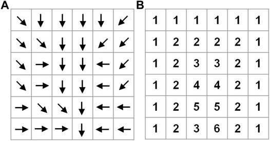
FIGURE 1. Flow direction (A) and different level of priority (B).
Following the prioritization of grid cells, ecohydrological modeling of different-level grid cells is implemented. The first level has the highest computation priority. Vegetation optimization is firstly conducted for the first-level grid cells and after vegetation parameters have been gained, ecohydrological processes of those grid cells are modeled. The outflow of those grid cells serves as the inflow of the downstream grid cells and accordingly participates in vegetation properties optimization of downstream grid cells. In this way, the lateral flow can be fully incorporated into vegetation optimality model.
The model test and evaluation are conducted in USDA-ARS Walnut Gulch Experimental Watershed (WGEW) near Tombstone, Arizona (Figure 2). The watershed is located in the upper San Pedro River Basin, covering 7,600 km2 in Sonora, Mexico and Arizona. The area of the WGEW is about 145 km2. The average annual temperature is about 17–19°C, and the average annual precipitation is 322 mm, with 67% rainfall in summer (Goodrich, et al., 2008). The primary vegetation of the watershed is grass and shrubs and is a transition zone between the Chihuahuan and Sonoran Deserts.
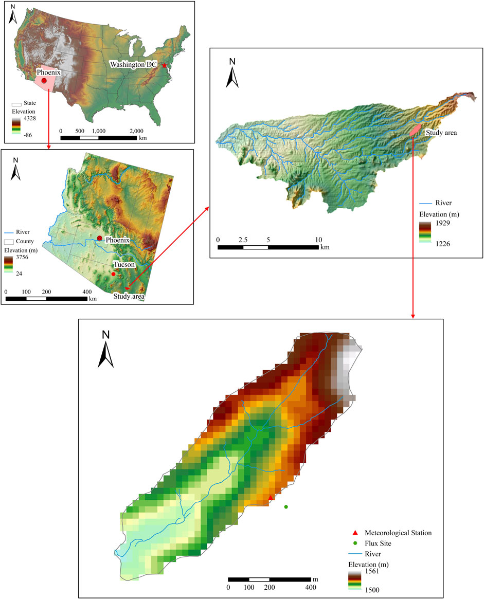
FIGURE 2. Location of study area and observation station.
We use a small watershed near the Kendall grass site (109°56′8″W, 31°44′10″N; elevation: 1,526 m) as the validation watershed (Figure 2). The watershed is small, with nearly unique climate, vegetation, and soil type, therefore, the spatial variability of modeled ET and GPP can be attributed to lateral flow.
Data used in this study are obtained from the Southwest Watershed Research Center (SWRC) of USDA through the official governmental website (http://www.tucson.ars.ag.gov/dap/) (Emmerich and Verdugo, 2008). These data include spatial data, model driving data, and model validation data (Table 1). Meteorological measurements include precipitation (except for 2002), air temperature, air humidity, Photosynthetically Active Radiation (PAR), solar radiation are gained from flux data near the Kendall grass site. Flux data are acquired from Bowen Ratio Energy Balance System (BREB, Model 023/CO2, Campbell Scientific Inc., Logan, UT). In the BREB system, atmospheric gradients of air temperature, moisture, and CO2, are measured every 10 s and averaged to 20 min. These measurements are scaled up to 1 h for model input. Precipitation data of 2002 is gained from the precipitation database of Walnut Gulch Raingages because precipitation of 2002 from flux data is much lower than that from raingage indicating there is missing observation of this year.

TABLE 1. Data used in this study.
The validation data including water vapor flux and CO2 flux are also acquired from Bowen Ratio Energy Balance System. Considering the quality and continuity of the data, the meteorological data from 1998-01-01 to 2007-12-31 are selected to force the DisVOM model.
The model only has the outcome of leaf photosynthesis, which can not be directly measured. In this study, as grass is the main vegetation in the ecosystem, we convert the measured Net Ecosystem Exchange (NEE) of CO2 through a flux-partition method into GPP and ecosystem respiration (Re) by the following equation.
As Re is explicitly dependent on air or soil temperature, Re can be estimated from observed temperature data using the exponential regression model (van’t Hoff, 1884)
Where a and b are fitting parameters, Ts is the soil temperature. As nighttime NEE values are equal to Re as GPP equals 0, therefore we can use the nighttime NEE (nighttime is defined as down solar radiation <1 W m-2) and soil temperature to estimate the parameters. Once the parameters are fitted, the daytime NEE can be computed (Figure 3).
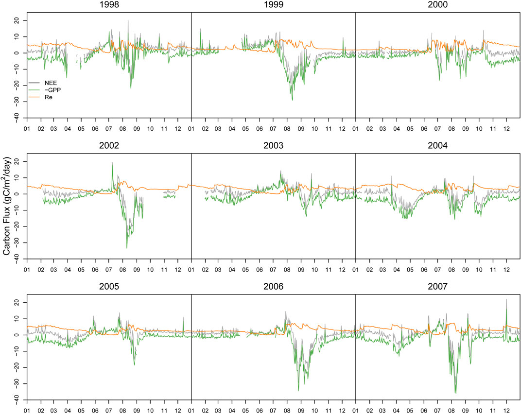
FIGURE 3. Subdivision of measured NEE into GPP and ecosystem respiration.
Based on the flow direction data (Figure 4A), prioritization of the grid cells are conducted as illustrated in Figure 4B. All the grid cells are partitioned into 45 layers. Grid cells of lower layers have higher priority, and grid cells in the same layer can model simultaneously.
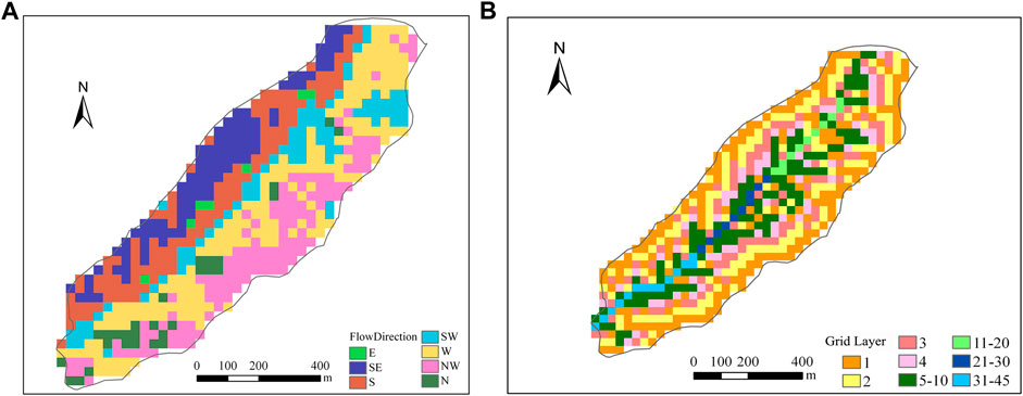
FIGURE 4. Flow direction (A) and prioritization of grid cells (B) in Kendall watershed.
Parameters for the optimality-based model consist of soil parameters (Table 2) and vegetation parameters. Soil parameters are specified according to Scott et al., 2000. In the VOM model, the soil profile is subdivided into sub-layers but the van Genuchten soil parameters of each layer are treated as one value. Therefore, we then average the soil parameters of each sub-layer from the work of Scott et al (2000) and obtain one value for the whole soil profile.
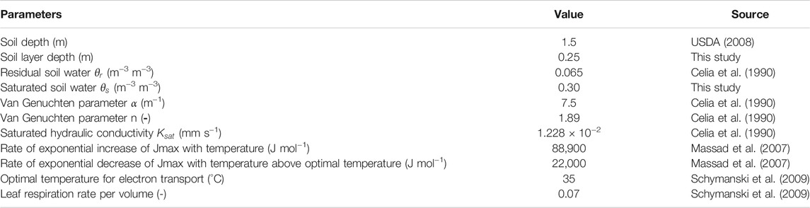
TABLE 2. Soil and vegetation parameters.
Most of the vegetation parameters in this study are derived from vegetation optimization. Some of the parameters that cannot be optimized are obtained from existing studies, as shown in Table 2. These parameters are prescribed according to the average value of C3 shrub from previous studies (Schymanski et al., 2009; Massad et al., 2007; Lei et al., 2009).
The simulated daily ET, soil water and GPP are compared with the measured at the Kendall grass site. As the flux measurements of 2001 are seriously absent, this year is removed for validation. A one-to-one comparison of simulated values and measurements is shown in Figure 5. Most of the points are distributed along the 1:1 line, indicating a good agreement between the observed data and simulated values.
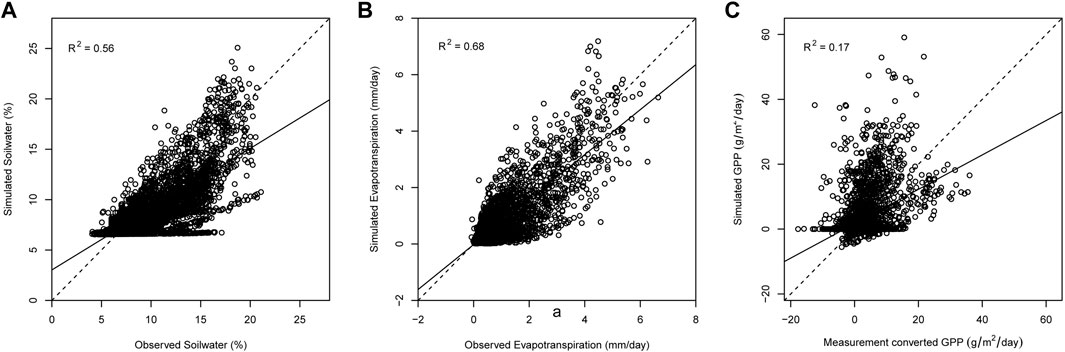
FIGURE 5. Scatters of simulated and measured ET (A), SW (B) and GPP (C).
Figure 6 illustrates the measured and simulated ET from 1998-2007 (except 2001). The simulated ET shows a similar seasonal dynamic pattern with measured ET. It indicates that the model can explain the variability of measured ET. As compared with precipitation data, we can see that the model captures the ET dynamic reasonably well in response to rainfall events. When precipitation occurs ET occurs and simulated ET is mainly concentrated in monsoon when rainfall concentrates. Root Mean Square Error (RMSE) of ET simulation is 0.57 mm/day, which is lower than the standard deviation of ET, 1.09 mm/day (Table 3). Figure 7 shows simulated daily evaporation and transpiration. Evaporation and transpiration both mainly occur in the monsoon following the precipitation events. Evaporation responds immediately to precipitation events, while transpiration shows a lagged response to those events. In spring or winter, ET is mainly dominated by evaporation, while in the monsoon, transpiration increases quickly after precipitation and dominates ET. These results are consistent with Emmerich and Verdugo (2008).
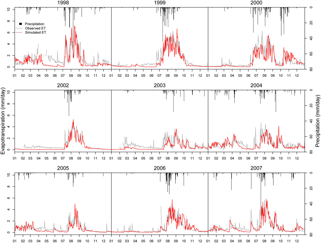
FIGURE 6. Comparison of simulated and observed daily ET.
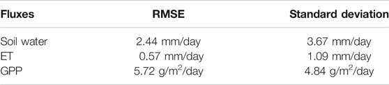
TABLE 3. Accuracy of simulation.
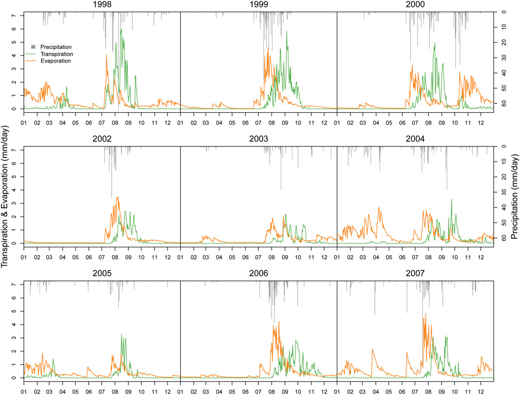
FIGURE 7. Comparison of simulated soil evaporation and transpiration.
Figure 8 shows the seasonal dynamic of measured and simulated soil water. Generally, the performance of soil water simulation is well. Soil water in the monsoon season is simulated pretty well with nearly the same peak and corresponding seasonal variation. Root Mean Square Error (RMSE) of soil water simulation is 2.44 mm/day, lower than the standard deviation of soil water, 3.67 mm/day (Table 3). However, there is a tendency to underestimate soil water in the spring, especially in those years with low spring precipitation (like 2005 and 2006). It might be because, as precipitation is relatively small, the model assumes vegetation is inactive, and roots are not developed, leading to low soil water restored.
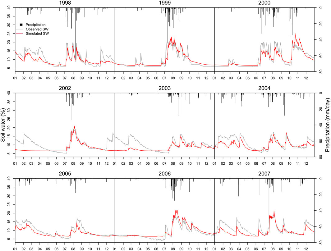
FIGURE 8. Comparison of simulated and observed daily soil water dynamic.
Figure 9 gives the simulated results of daily GPP and NEE-partitioned GPP. Generally, the performance of GPP simulation is acceptable. Simulated GPP shows the same patterns with NEE-partitioned GPP in most years. RMSE of GPP simulation is 5.72 g/m2/day, which is slightly higher than the standard deviation of GPP, 4.84 g/m2/day (Table 3). However, we also find a tendency to underestimate GPP in some years. It might be due to the unreasonable prediction of vegetation cover as it underestimates vegetation in the non-growing season.
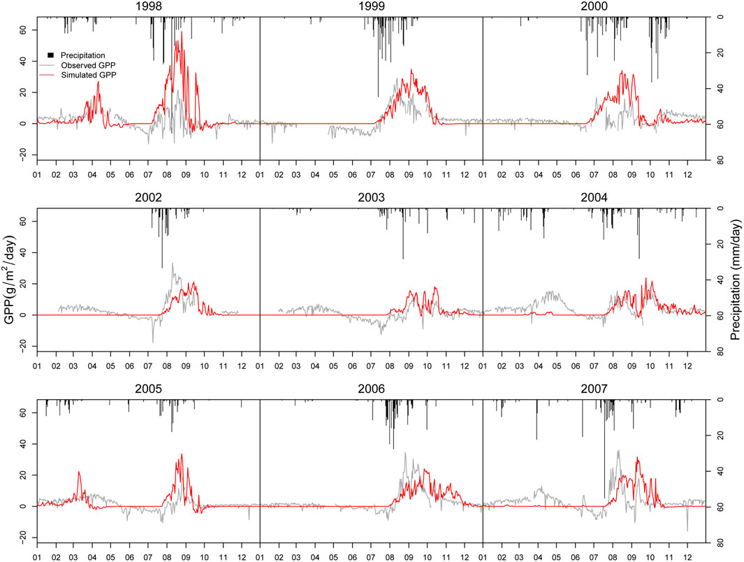
FIGURE 9. Comparison of simulated daily GPP and NEE-partitioned GPP.
Figure 10 shows the spatial distributions of annual ET and GPP of DisVOM (Figure 10) for 1999. The spatial variations of ET and GPP exhibit nearly identical patterns. Comparing the distribution of slope and Topographic Wetness Index (TWI) (Figure 11), we can find that the spatial distribution of annual ET and GPP of DisVOM demonstrates similar patterns with slope and TWI. Grid cells with high slopes tend to have low ET and GPP, while grid cells with low slopes tend to have high ET and GPP. Grid cells with high TWI are inclined to have high ET and GPP, while grid cells with low TWI appear to have low ET and GPP.
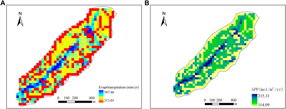
FIGURE 10. Spatial distribution of ET (A) and GPP (B) simulated by DisVOM and VOM.
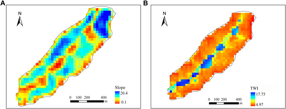
FIGURE 11. Spatial distribution of slope (A) and TWI (B) of Kendall watershed.
ET and GPP of all grid cells in the watershed are sorted and divided into eight groups to quantitatively analyze the correlation between simulated ET and GPP with slope and TWI. The averaged value of ET, GPP, slope and TWI of each group is estimated. As illustrated in Figure 12, ET and GPP show a significant negative correlation with slope and positive correlation with TWI. Annual ET and GPP decreased with the increase of slope. Annual ET and GPP increase with the increase of TWI.
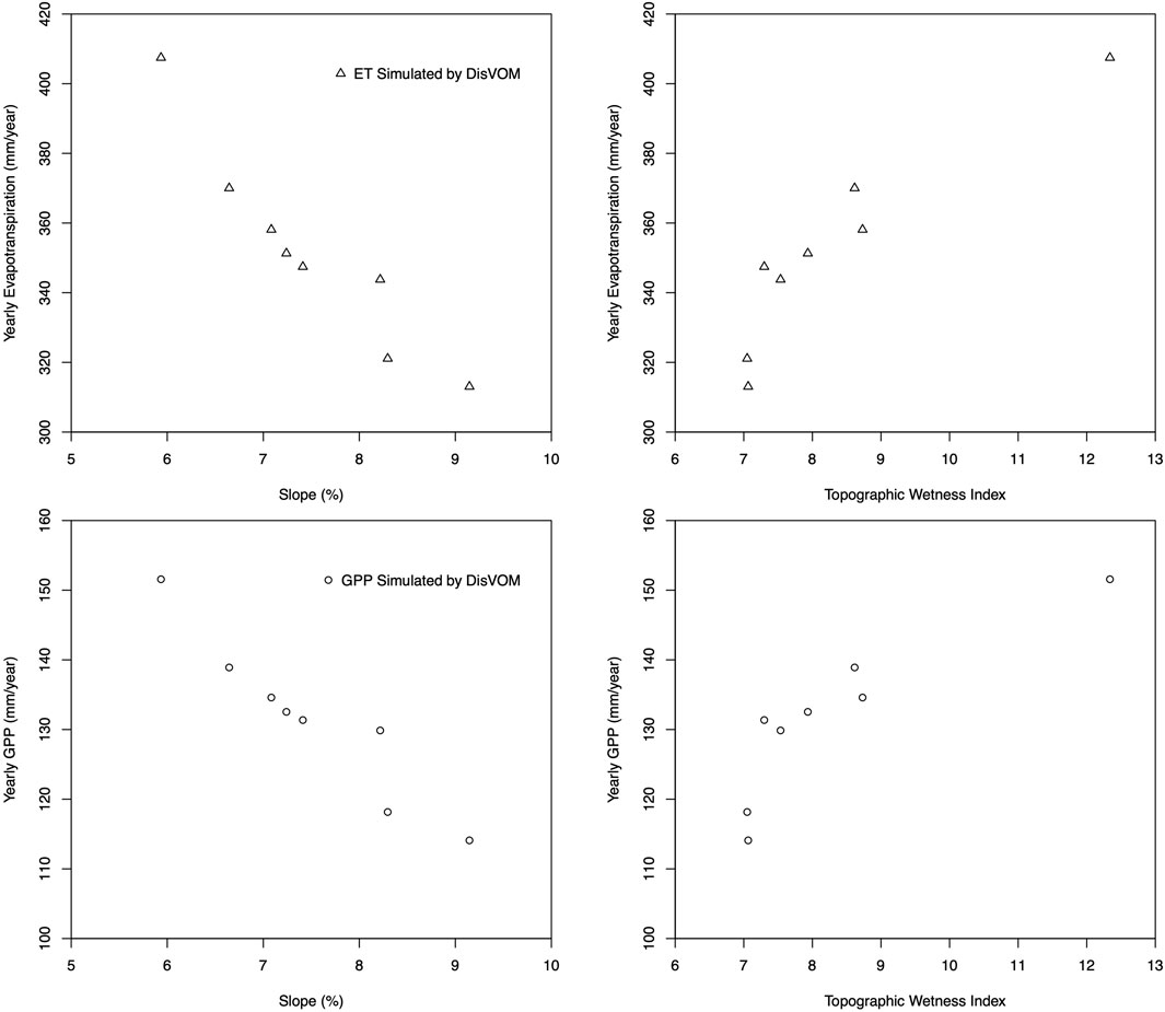
FIGURE 12. Correlation of annual ET and GPP with slope and TWI.
In general, the spatial pattern of annual ET and GPP reflect the fundamental impact of topographical controls on soil water and root water uptake. The lower portions of the watershed have higher soil water content due to the above recharge. Grass could develop high root density in those areas and consequent high transpiration and carbon assimilation. It is the truth, as in water-limited ecosystems, water is a scarce resource for plants and plays a fundamental role in vegetation dynamics, such as canopy property and root density. The DisVOM model can discriminate the effect of topography on redistribution of precipitation into soil water and the consequent variations in ET and carbon assimilation.
This paper presents an optimality-based watershed ecohydrological model. The model subdivided watershed into grid cells. On each grid cell, an optimality-based ecohydrological model, VOM is applied to describe the vertical water and vegetation mutual interactions. Overland flow is incorporated to the VOM model to simulate soil water redistribution and subsequently modify vegetation properties optimization. A hierarchical strategy is developed to integrate lateral flow to VOM model, which prioritizes the grid cells of the watershed into different levels according to the dependency of grid cells. The model is tested in the Walnut Gulch watershed and demonstrates good consistency with site measurements. However, there are still some limitations of this study, which can be summarized as follows.
The model demonstrates good performance in growing season, however, evident discrepancies arise during winter and spring. This is probably, to a great degree, attributed to the underestimation of soil water.
As we look into the precipitation data and compare spring soil water of different years, one possible reason might be the undocumented precipitation. For 2002, we utilize the data from rain gauge, because precipitation measurement of flux is lower. However, there was no rain in the spring of 2002, which is unrealistic. In contrast, from the flux data we find a small amount of precipitation. Besides, we compare observed soil water of two period 2002.12-2003.05 and 2007.01-2007.05. The two periods have quite similar soil water with respect to similar amount, shape and peak. However, measured precipitation in 2002.12–2003.05 is considerably lower than precipitation of 2007.01–2007.05. As there is no precipitation for nearly 2 months for both periods, antecedent soil moisture is nearly the same for the two periods. Hence, it is unlikely to have the same soil water with dramatically different amount of precipitation.
Another possible reason might be the uniform setting of soil profile. In the model, soil profile is subdivided into sub-layers with same depth (25 cm). According to the previous study in this area, vertical soil properties vary dramatically (Scott et al., 2000). For example, saturated hydraulic conductivity of the top layer (0–4 cm) is about 31.1 cm/day, 18.7 cm/day for the second layer (4–9 cm), 7.2 cm/day for the third layer (9–16 cm), 8.5 cm/day for the third layer (16–35 cm), 8.7 cm/day for the third layer (35–62 cm), and 36.9 cm/day for the bottom layer (62–150 cm). For the layers near surface, a depth of 25 cm is unable to characterize the variation of soil properties, which could attributed to the underestimation of soil water in the non-growing season when root uptake of vegetation is low.
There are some inconsistent of GPP for some years especially in the non-growing season. For 2002, 2003, 2004, and 2007, grass grew in the spring as there is GPP partitioned from NEE, but from the model there is no grass grew as GPP is little. This is possibly caused by the underestimation of soil water. As stated in 4.1, soil water is dramatically underestimated, so the available water for root water uptake is low. This might directly influence root development and leaf growth, leading to low simulated carbon assimilation.
Another reason is that there is no directed measured GPP. GPP separated from NEE measurements are used for validation. Not only the NEE measurements are highly associated with measurement error, but also the NEE separation is associated with uncertainty (Raj, et al., 2016). This might contributed partly to the inconsistent of simulated and observed GPP comparison.
Another problem of this study is that the model only considers overflow routing, subsurface flow and ground water is not simulated. Therefore it can’t give stream flow as the other two components are neglected. The main concern of this study is to explore whether incorporated a kind of lateral flow could alter the soil water redistribution and influence vegetation-soil-water mutual interaction and coevolution. Incorporation of subsurface flow and ground water would otherwise require much more parameters which need to be calibrated. Although VOM model has the unique merit that it does not need prior vegetation properties as input, we still find environment parameters (such as topography, soil), associated with hydrological processes are difficult to determine. Calibration might need for hydrological processes. Nevertheless, the lateral flow of the current model is simple and it is unrealistic without simulating the other component of stream flow. We will integrate subsurface flow and ground water to the model in the future and learn the method from big data science for hydrological parameters estimation (Liu et al., 2017; Zhang et al., 2021).
Despite the above issues, the model presents in this study is capable of predicting ET, soil water, and GPP reasonably well, for most of years, especially for the growing season. The seasonal dynamic of ET, soil water, and GPP demonstrate good consistency with observations. The model produces reasonable spatial distribution of ET and GPP, indicating it is able to capture the influence of lateral flow on water redistribution, vegetation dynamic and so on. It can be concluded that the model effectively extends VOM from field scale to watershed scale and could be a useful tool assessing the impact of climate change and human activities on vegetation and water cycle.
Publicly available datasets were analyzed in this study. This data can be found here: http://www.tucson.ars.ag.gov/dap/.
LC carried out model development, tested the model, analyzed the results, and drafted the manuscript. ZH participated in collecting and processing some of the data for model validation. XD provided fundamental suggestions for this study. MYAK reviewed and revised the manuscript. XL and JW processed some of the figures, and revised the manuscript.
This study is supported by Open Research Fund Program of State key Laboratory of Hydroscience and Engineering (sklhse-2021-A-01), Water Conservancy Science and Technology Innovation Project in Guangdong Province (No. 202012), National Key R&D Program of China (No. 2018YFC1508103), Strategic Priority Research Program of the Chinese Academy of Sciences (XDA 19080103), Innovation Drive Development Special Project of Guangxi (GuikeAA20302022).
Author XL was employed by company China Water Northeastern Investigation, Design and Research Co., Ltd.
The remaining authors declare that the research was conducted in the absence of any commercial or financial relationships that could be construed as a potential conflict of interest.
All claims expressed in this article are solely those of the authors and do not necessarily represent those of their affiliated organizations, or those of the publisher, the editors and the reviewers. Any product that may be evaluated in this article, or claim that may be made by its manufacturer, is not guaranteed or endorsed by the publisher.
Amein, M., and Fang, C. S. (1969). Stream Flow Routing (With Applications to North Carolina Rivers), Report No. 17. Raleigh, NC: Water Resources Research Institute of the University of North Carolina.
Ball, J. T., Woodrow, I. E., and Berry, J. A. (1987). “A Model Predicting Stomatal Conductance and its Contribution to the Control of Photosynthesis under Different Environmental Conditions,” in Progress in Photosynthesis Research (Dordrecht: Martinus Nijhoff Publishers), 221–224. doi:10.1007/978-94-017-0519-6_48
Band, L. E., Patterson, P., Nemani, R., and Running, S. W. (1993). Forest Ecosystem Processes at the Watershed Scale: Incorporating Hillslope Hydrology. Agric. For. Meteorology 63, 93–126. doi:10.1016/0168-1923(93)90024-c
Berninger, F., Mäkelä, A., and Hari, P. (1996). Optimal Control of Gas Exchange during Drought: Empirical Evidence. Ann. Bot. 77, 469–476. doi:10.1006/anbo.1996.0057
Biederman, J. A., Scott, R. L., Bell, T. W., Bowling, D. R., Dore, S., Garatuza‐Payan, J., et al. (2017). CO 2 Exchange and Evapotranspiration across Dryland Ecosystems of Southwestern North America. Glob. Change Biol. 23 (10), 4204–4221. doi:10.1111/gcb.13686
Cabon, A., Martínez-Vilalta, J., Martínez de Aragón, J., Poyatos, R., and De Cáceres, M. (2018). Applying the Eco-Hydrological Equilibrium Hypothesis to Model Root Distribution in Water-Limited Forests. Ecohydrology 11 (7), e2015. doi:10.1002/eco.2015
Caylor, K. K., Scanlon, T. M., and Rodriguez-Iturbe, I. (2009). Ecohydrological Optimization of Pattern and Processes in Water-Limited Ecosystems: A Trade-Off-Based Hypothesis. Water Resour. Res. 45, W08407. doi:10.1029/2008WR007230
Caylor, K. K., Scanlon, T. M., and Rodriguez-Iturbe, I. (2004). Feasible Optimality of Vegetation Patterns in River Basins. Geophys. Res. Lett. 31, a–n. doi:10.1029/2004GL020260
Celia, M. A., Bouloutas, E. T., and Zarba, R. L. (1990). A General Mass-Conservative Numerical Solution for the Unsaturated Flow Equation. Water Resour. Res. 26 (7), 1483–1496. doi:10.1029/wr026i007p01483
Cevza, M. K., Miguel, A., Medina, J., and Rao, P, (2005). On Numerical Modeling of Overland Flow. Appl. Maths. Comput. 166, 724–740. doi:10.1016/j.amc.2004.06.063
Chen, L., Sun, L., Liu, W., Wang, L., Wu, H., Zhu, A.-X., et al. (2019). Evapotranspiration Partitioning Using an Optimality-Based Ecohydrological Model in a Semiarid Shrubland. Int. J. Digital Earth 12 (12), 1423–1440. doi:10.1080/17538947.2018.1503741
Chen, L., Wang, L., Ma, Y., and Liu, P. (2015). Overview of Ecohydrological Models and Systems at the Watershed Scale. IEEE Syst. J. 9 (3), 1091–1099. doi:10.1109/jsyst.2013.2296979
Cowan, I. R., Farquhar, G. D., and Jennings, D. H. (1977). “Stomatal Function in Relation to Leaf Metabolism and Environment,” in Integration of Activity in the Higher Plant (Cambridge: Cambridge University Press).
Cowan, I. R. (2002). Fit, Fitter, Fittest: Where Does Optimization Fit in? Silva Fennica 36 (3), 744–754. doi:10.14214/sf.536
De Boer, H. J., Lammertsma, E. I., Wagner-Cremer, F., Dilcher, D. L., Wassen, M. J., and Dekker, S. C. (2011). Climate Forcing Due to Optimization of Maximal Leaf Conductance in Subtropical Vegetation under Rising CO2. Proc. Natl. Acad. Sci. 108 (10), 4041–4046. doi:10.1073/pnas.1100555108
Duan, Q. Y., Sorooshian, S., and Gupta, V. K. (1994). Optimal Use of the SCE-UA Global Optimization Method for Calibrating Watershed Models. J. Hydrol. 158 (3-4), 265–284. doi:10.1016/0022-1694(94)90057-4
Eagleson, P. S. (2002). Ecohydrology: Darwinian Expression of Vegetation Form and Function. Cambridge: Cambridge University Press.
Eagleson, P. S. (1978). Climate, Soil, and Vegetation: 1. Introduction to Water Balance Dynamics. Water Resour. Res. 14 (5), 705–712. doi:10.1029/wr014i005p00705
Emmerich, W. E., and Verdugo, C. L. (2008). Long-term Carbon Dioxide and Water Flux Database, Walnut Gulch Experimental Watershed, Arizona, United States. Water Resour. Res. 44, W05S09. doi:10.1029/2006WR005693
Fatichi, S., Pappas, C., and Ivanov, V. Y. (2016). Modeling Plant-Water Interactions: an Ecohydrological Overview from the Cell to the Global Scale. WIREs Water 3 (3), 327–368. doi:10.1002/wat2.1125
Franklin, O., Harrison, S. P., Dewar, R., Farrior, C. E., Brännström, Å, Dieckmann, U., et al. (2020). Organizing Principles for Vegetation Dynamics. Nat. Plants 6 (5), 444–453. doi:10.1038/s41477-020-0655-x
Gao, H., Birkel, C., Hrachowitz, M., Tetzlaff, D., Soulsby, C., and Savenije, H. H. G. (2019). A Simple Topography-Driven and Calibration-free Runoff Generation Module. Hydrol. Earth Syst. Sci. 23, 787–809. doi:10.5194/hess-23-787-2019
Gao, H., Hrachowitz, M., Schymanski, S. J., Fenicia, F., Sriwongsitanon, N., and Savenije, H. H. G. (2014). Climate Controls How Ecosystems Size the Root Zone Storage Capacity at Catchment Scale. Geophys. Res. Lett. 41 (22), 7916–7923. doi:10.1002/2014gl061668
Goodrich, D. C., Keefer, T. O., and Unkrich, C. L., (2008). Smith Long-Term Precipitation Database, Walnut Gulch Experimental Watershed, Arizona, United States. Water Resour. Res. 44, W05S04. doi:10.1029/2006R00578210.1029/2006wr005782
Govind, A., Chen, J. M., Margolis, H., Ju, W., Sonnentag, O., and Giasson, M.-A. (2009). A Spatially Explicit Hydro-Ecological Modeling Framework (BEPS-TerrainLab V2.0): Model Description and Test in a Boreal Ecosystem in Eastern North America. J. Hydrol. 367, 200–216. doi:10.1016/j.jhydrol.2009.01.006
Huang, F., Mo, X., Hu, S., and Li, L. (2020). Agricultural Water Optimization Coupling with a Distributed Ecohydrological Model in a Mountain-plain basin. J. Hydrol. 590, 125336. doi:10.1016/j.jhydrol.2020.125336
Hwang, T., Band, L., and Hales, T. (2009). Ecosystem Processes at the Watershed Scale: Extending Optimality Theory from Plot to Catchment. Water Resour. Res. 45, W11425. doi:10.1029/2009WR007775
Ivanov, V. Y., Bras, R. L., and Vivoni, E. R. (2008). Vegetation-hydrology Dynamics in Complex Terrain of Semiarid Areas: 1. A Mechanistic Approach to Modeling Dynamic Feedbacks. Water Resour. Res. 44, W03429. doi:10.1029/2006WR00558810.1029/2006wr005588
Keefer, T. O., Moran, M. S., and Paige, G. B. (2008). Long-term Meteorological and Soil Hydrology Database, Walnut Gulch Experimental Watershed, Arizona, United States. Water Resour. Res. 44, W05S07. doi:10.1029/2006WR00570210.1029/2006wr005702
Kuppel, S., Tetzlaff, D., Maneta, M. P., and Soulsby, C. (2018). What Can We Learn from Multi-Data Calibration of a Process-Based Ecohydrological Model? Environ. Model. Softw. 101, 301–316. doi:10.1016/j.envsoft.2018.01.001
Lei, H., Yang, D., Schymanski, S. J., and Sivapalan, M. (2009). Modeling the Crop Transpiration Using an Optimality-Based Approach. Sci. China Ser. E-technol. Sci. 51 (S2), 60–75. doi:10.1007/s11431-008-6008-z
Liu, P., Zhang, H., and Eom, K. B. (2017). Active Deep Learning for Classification of Hyperspectral Images. IEEE J. Sel. Top. Appl. Earth Observations Remote Sensing 10 (2), 712–724. doi:10.1109/jstars.2016.2598859
Massad, R. S., Tuzet, A., and Bethenod, O. (2007). The Effect of Temperature on C(4)-type Leaf Photosynthesis Parameters. Plant Cel Environ 30 (10), 1191–1204. doi:10.1111/j.1365-3040.2007.01691.x
Pauwels, V. R. N., Verhoest, N. E. C., De Lannoy, G. J. M., Guissard, V., Lucau, C., and Defourny, P. (2007). Optimization of a Coupled Hydrology-Crop Growth Model through the Assimilation of Observed Soil Moisture and Leaf Area index Values Using an Ensemble Kalman Filter. Water Resour. Res. 43. doi:10.1029/2006WR004942
Raj, R., Hamm, N. A. S., Tol, C. v. d., and Stein, A. (2016). Uncertainty Analysis of Gross Primary Production Partitioned from Net Ecosystem Exchange Measurements. Biogeosciences 13 (5), 1409–1422. doi:10.5194/bg-13-1409-2016
Rice, J. S., and Emanuel, R. E. (2019). Ecohydrology of Interannual Changes in Watershed Storage. Water Resour. Res. 55 (10), 8238–8251. doi:10.1029/2019wr025164
Rodriguez-Iturbe, I., D'Odorico, P., Porporato, A., and Ridolfi, L. (1999). On the Spatial and Temporal Links between Vegetation, Climate, and Soil Moisture. Water Resour. Res. 35, 3709–3722. doi:10.1029/1999wr900255
Rodriguez-Iturbe, I.,, and Porporato A. (Editors) (2005). “Ecohydrology of Water Controlled Ecosystems: Soil Moisture and Plant Dynamics,” (London: Cambridge University Press).
Schymanski, S. J., Sivapalan, M., Roderick, M. L., Beringer, J., and Hutley, L. B. (2008). An Optimality-Based Model of the Coupled Soil Moisture and Root Dynamics. Hydrol. Earth Syst. Sci. 12 (3), 913–932. doi:10.5194/hess-12-913-2008
Schymanski, S. J., Sivapalan, M., Roderick, M. L., Hutley, L. B., and Beringer, J. (2009). An Optimality-Based Model of the Dynamic Feedbacks between Natural Vegetation and the Water Balance. Water Resour. Res. 45. doi:10.1029/2008WR006841
Scott, R. L., Shuttleworth, W. J., Keefer, T. O., and Warrick, A. W. (2000). Modeling Multiyear Observations of Soil Moisture Recharge in the Semiarid American Southwest. Water Resour. Res. 36 (8), 2233–2247. doi:10.1029/2000wr900116
Sivapalan, M. (2009). The Secret to 'doing Better Hydrological Science': Change the Question! Hydrol. Process. 23 (9), 1391–1396. doi:10.1002/hyp.7242
Speich, M. J. R., Lischke, H., and Zappa, M. (2018). Testing an Optimality-Based Model of Rooting Zone Water Storage Capacity in Temperate Forests. Hydrol. Earth Syst. Sci. 22 (7), 4097–4124. doi:10.5194/hess-22-4097-2018
Van der Tol, C., MeestersDolman, A. G. C. A. A. J., Dolman, A. J., and Waterloo, M. J. (2008). Optimum Vegetation Characteristics, Assimilation, and Transpiration during a Dry Season: 1. Model Description. Water Resour. Res. 44 (3), W03421. doi:10.1029/2007WR006241
Van’t Hoff, J. H. (1884). Etudes de dynamique chimique (studies of Chenmical dynamics). Amsterdam, Netherlands: Frederik Muller and Co.
Wang, C., Fu, B., Zhang, L., and Xu, Z. (2019). Soil Moisture-Plant Interactions: an Ecohydrological Review. J. Soils Sediments 19 (1), 1–9. doi:10.1007/s11368-018-2167-0
Xia, J., Zhang, Y., Mu, X., Zuo, Q., Zhou, Y., and Zhao, G. (2021). A Review of the Ecohydrology Discipline: Progress, Challenges, and Future Directions in China. J. Geogr. Sci. 31, 1085–1101. doi:10.1007/s11442-021-1886-0
Keywords: ecohydrology, ecohydrological modeling, vegetation optimality, lateral hydrological processes, spatial explicit
Citation: Chen L, Hu Z, Du X, Khan MYA, Li X and Wen J (2022) An Optimality-Based Spatial Explicit Ecohydrological Model at Watershed Scale: Model Description and Test in a Semiarid Grassland Ecosystem. Front. Environ. Sci. 10:798336. doi: 10.3389/fenvs.2022.798336
Received: 20 October 2021; Accepted: 05 January 2022;
Published: 21 February 2022.
Edited by:
Yizhe Zhan, MetService, New ZealandReviewed by:
Shi Hu, Institute of Geographic Sciences and Natural Resources Research (CAS), ChinaCopyright © 2022 Chen, Hu, Du, Khan, Li and Wen. This is an open-access article distributed under the terms of the Creative Commons Attribution License (CC BY). The use, distribution or reproduction in other forums is permitted, provided the original author(s) and the copyright owner(s) are credited and that the original publication in this journal is cited, in accordance with accepted academic practice. No use, distribution or reproduction is permitted which does not comply with these terms.
*Correspondence: Xiaoping Du, ZHV4cEBhaXJjYXMuYWMuY24=
Disclaimer: All claims expressed in this article are solely those of the authors and do not necessarily represent those of their affiliated organizations, or those of the publisher, the editors and the reviewers. Any product that may be evaluated in this article or claim that may be made by its manufacturer is not guaranteed or endorsed by the publisher.
Research integrity at Frontiers
Learn more about the work of our research integrity team to safeguard the quality of each article we publish.