Random Forest Classification Method for Predicting Intertidal Wetland Migration Under Sea Level Rise

Intertidal wetlands such as mangrove and saltmarsh are increasingly susceptible to areal losses related to sea level rise. This exposure is potentially offset by processes that might enable wetlands to accrete in situ or migrate landward under sea level rise, and planning policies that might open new opportunities for migration. We present and demonstrate a method to predict intertidal wetland distribution in the present-day landscape using random forest classification models, and use these models to predict the intertidal wetland distribution in future landscapes under specified sea level scenarios. The method is demonstrably robust in predicting present-day intertidal wetland distribution, with moderate correlation or better between predicted and mapped wetland distributions occurring in nearly all estuaries and strong correlation or better occurring in more than half of the estuaries. Given the accuracy in predicting present-day wetland distribution the method is assumed to be informative in predicting potential future wetland distribution when combined with best available models of future sea level. The classification method uses a variety of hydro-geomorphological surrogates that are derived from digital elevation models, Quaternary geology or soils mapping and land use mapping, which is then constrained by a representation of the future sea level inside estuaries. It is anticipated that the outputs from applying the method would inform assessments of intertidal wetland vulnerability to sea level rise and guide planning for potential wetland migration pathways.

1 Introduction

Coastal wetlands provide several important ecological services, including the provision of habitat, sediment stabilisation, carbon sequestration, and nutrient cycling (Barbier et al., 2011). These intertidal habitats are under pressure from numerous threats including coastal development, deforestation, aquaculture, weed invasion, damage by domestic and feral animals, climate change and sea level rise (e.g., Adam, 2009; Osland et al., 2016; Rogers et al., 2016; Gabler et al., 2017). The former pressures manifest in detail at the local scale whereas the latter two are regional in their impact.

Impacts to wetlands from climate change will be manifold, relating to increases in temperature and CO₂, the frequency and intensity of storms and changes in rainfall patterns which in turn may affect soil salinity (Ross and Adam, 2013). Sea level rise (SLR) is, however, the most obvious and well-studied future impact on coastal wetlands, with three broad scenarios recognised at the estuary scale: 1) no change to the present-day wetlands because they accumulate sediment at a rate that matches regional SLR; 2) a net increase in the wetland area as suitable new areas become inundated and offset any losses; and 3) a net decrease in wetland area because losses through drowning and/or erosion by increased wave energy exceed potential gains from sedimentation or migration (e.g., Morris et al., 2002; Woodroffe and Davies, 2009; Kirwan and Megonigal 2013; Spencer et al., 2016; Schuerch et al., 2018; Rogers et al., 2019). The latter scenario, where migration potential is limited by land development or topography, is termed “coastal squeeze” (Townend and Pethick, 2002; Borchert et al., 2018). Intertidal wetlands are typically found in narrow sections of coastline fringing estuaries where there has also been substantial human modification to the coastlines. As such, foreshore structures may substantially influence the ability of wetlands to migrate with SLR (Ross and Adam 2013). This broad range in potential response of coastal wetlands to SLR makes it challenging to assess regional vulnerability.

In their investigation spanning sixteen estuaries and six states in the United States, Raposa et al. (2016) identified ten metrics, including rate of SLR, tidal range, sediment supply and a variety of topographic factors that contribute to tidal marsh resilience. Applying thresholds to each metric to obtain scores, they integrated the metrics into an overall resilience index to inform their vulnerability assessment. The metrics were all founded upon continuous spatial data layers and the vulnerability index could be uniformly mapped across the estuary. In a regional scale study of 39 estuaries along the US Gulf of Mexico coast, Borchert et al. (2018) determined the lateral accommodation space under three SLR scenarios (0.5, 1.0, and 1.5 m). Like the previous study, all the foundational data were spatial layers thus allowing continuous mapping of both barriers and opportunities for wetland migration. Doughty et al. (2018) evaluated the regional resiliency of coastal wetlands in Southern California, United States by associating migration potential with wetland hypsometry determined from digital elevation models (DEMs). Similarly, in their investigation of Chesapeake Bay, United States Molino et al. (2021) used the land slope at the inner boundary of saltmarsh to assess potential saltmarsh migration under SLR. While the three abovementioned scenarios of wetland response to sea level rise are complex and depend on numerous factors manifesting at nested scales, the potential for upslope wetland migration is widely recognised as an important component of any assessment of wetland vulnerability to SLR (e.g., Borchert et al., 2018; Doughty et al., 2018; Molino et al., 2021).

Statistical learning models such as random forest (RF) regression and classification techniques have been used previously in a variety of wetland research. For example, RF regression has been used to estimate biomass density in wetlands from WorldView-2 imagery (Mutanga et al., 2012). Similarly, RF classification has been used to delineate wetland areas for mapping wetland extent from a range of remotely sensed imagery (e.g., Corcoran et al., 2013; Felton et al., 2019), and for classifying and mapping the distribution of wetland types (e.g., Dubeau et al., 2017; Mahdianpari et al., 2017). In a recent study Wen and Hughes (2020) demonstrated the value of RF classification over a variety of machine learning techniques for mapping wetland vegetation in the Manning River estuary, New South Wales, Australia. To the best of our knowledge, however, RF-models developed to predict present-day distribution of intertidal wetlands have not been applied to predict their future distribution under sea level rise.

The aim of this paper is to demonstrate a new RF classification-based method, applicable at the regional/jurisdictional scale, for predicting potential areas that mangrove and saltmarsh might migrate to in the future landscape under SLR. First, we build a RF-model for each estuary using the map of current mangrove and saltmarsh distribution. The RF-models establish the hydro-geomorphological conditions for existing wetlands based on a set of surrogate variables. We then predict the future distribution of coastal wetlands under three SLR scenarios: + 0.5 m, + 1.0 m, and + 1.5 m. The first two scenarios are indicative of the range of SLR projections for southeast Australia out to the year 2100 under RCP 8.5 and the latter scenario is likely to be exceeded beyond 2100 (Hanslow et al., 2018). Finally, the distributions of wetlands are predicted under three land use constraint scenarios: limited (migration is constrained within protected lands such as reserves and natural conservation parks), intermediately constrained (low intensity land uses such as grazed native vegetation are available), and no limitation (all lands except urban settlements are available for wetlands). The outcome of implementing this method is maps of future mangrove and saltmarsh distribution that can inform regional/jurisdictional scale assessments of intertidal wetland vulnerability to sea level rise.

2 Materials

2.1 Data Sources and Preparation

2.1.1 Response Variables

A variety of coastal saline wetlands exist in NSW, including salt flats, saltmarsh, mangrove, tidal sand and mud flats and seagrass. The three macrophyte-dominated wetlands are the only ones that are mapped for natural resource management purposes, and seagrass primarily occupies a subtidal position in the landscape thus requiring a unique set of predictor variables. We therefore focussed here on the occurrence of intertidal mangrove and saltmarsh wetlands as the response variables (Table 1).

TABLE 1

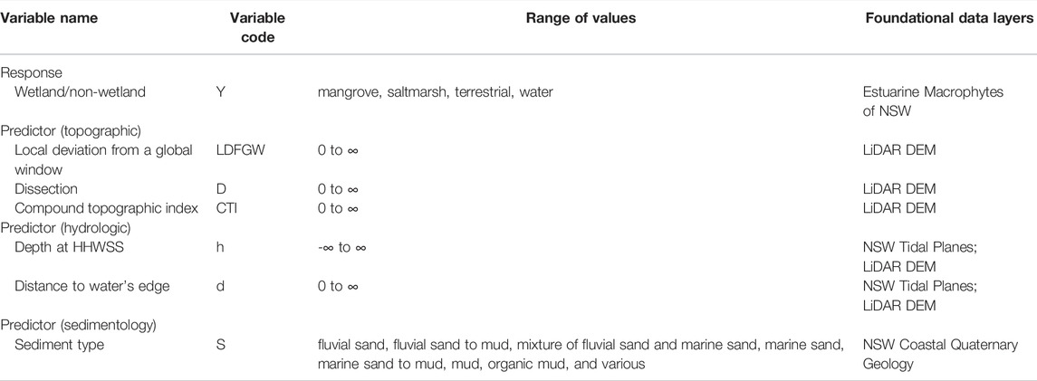
TABLE 1. List of model variables.

In developing the model for predicting present-day distribution of mangrove and saltmarsh, we used existing macrophyte maps produced by the NSW Department of Primary Industries (Fisheries), which are available online as the Estuaries (including macrophyte detail) Data Set (https://datasets.seed.nsw.gov.au/dataset/estuaries-including-macrophyte-detail5ebff). High resolution aerial imagery was used to map wetlands using Object Based Image Analysis (Trimble eCognition), followed by field validation. Species of mangrove and saltmarsh are not discriminated in the habitat maps and polygons are classified as being dominated by either mangrove or saltmarsh. Spatially balanced random samples of mapped mangrove or saltmarsh were extracted using ArcMap 10.4 (ESRI, Redlands, CA, United States). The number of samples within each patch of mangrove or saltmarsh was determined by the area of the polygon. To ensure that the random samples extracted had a unique set of environmental variables we restricted the distance between neighbouring points to be greater than 5 m. Samples were also selected in adjacent areas that were not mapped as either mangrove or saltmarsh and these were called water or background. Water was defined as the present-day extent of estuary excluding mapped mangrove and saltmarsh. Background was defined as the present-day mapped area of land, excluding mapped mangrove and saltmarsh, that extends to the maximum inundation extent for the largest SLR scenario considered here; i.e., + 1.5 m. Note that does not simply mean the contour that is 1.5 m above present water level throughout the estuary, because we have used a tidal plane approach rather than the simplistic bathtub approach for projecting future water levels inside the estuaries (see Section 2.1.2).

Many of the estuary catchments in NSW have been partially or totally cleared and developed, for example, it is estimated that the distribution of saltmarsh has been reduced by 80% as a result of development in the Sydney region (Stricker, 1995; Saintilan and Williams, 2000). To avoid any model bias toward “background” areas, it was therefore necessary to exclude land use types representative of human activities that may include previously cleared areas of mangrove and saltmarsh (e.g., cropland, irrigated pastures, forest plantation, residential areas) when generating background points. Land use maps produced by the NSW Department of Planning Industry and Environment, which are available online as NSW Landuse 2017 (https://data.nsw.gov.au/data/dataset/nsw-landuse-2017) were used to extract a random sample of background points. These points were only sampled from natural and semi-natural land cover that are neither saltmarsh nor mangrove.

2.1.2 Predictor Variables

The choice of predictor variables was determined by 1) their relevance to processes controlling the position of mangrove and saltmarsh in the landscape; and 2) their availability as a state-wide spatial data set.

Topographic variables—The state-wide 5 m digital elevation model (DEM) used here was derived from airborne light detection and ranging (LiDAR) surveys covering the entire coastal area with a nominal vertical accuracy of 0.15 m. The DEM was used to derive raster layers representing three topographic predictor variables (Table 1). The local deviation from a global window, LDFGW, was calculated using

$LDFG{W}_i=\overline{y}-y_i$

where $\overline{y}$ is the evaluated mean of the 3 by 3 window, and $y_i$ is the elevation of the focus grid. The dissection, D, describes the surface texture and was calculated using

$D_i=\frac{y_i-y_{min}}{y_{max}-y_{min}}$

where $y_i$ is the elevation of the focus grid and $y_{max}$ and $y_{min}$ are the maximum and minimum elevations within the 3 by 3 window. The compound topographic index, CTI, is a steady-state wetness index (Moore et al., 1991) representing both the upstream contributing area per unit width orthogonal to the flow direction, A, and the surface slope, tanβ in radians, and was calculated using

$CTI=\ln \left(\frac{A}{\tan \beta }\right)$

These DEM-derived variables are expected to represent the typical morphology of present-day mangrove and saltmarsh wetlands as approximately planar (and shallow basins), with horizontal to gently dipping surfaces that receive overland flow and are poorly drained.

Sedimentological variables—Mangroves generally require soft and fine-grained substrates to develop (Galloway, 1982), and sediment type affects the condition and growth of saltmarsh (Adam, 1978), suggesting that sedimentological variables would also be useful predictors of distribution. We used the NSW Coastal Quaternary Geology Data Package (Troedson, 2015) to create a raster of sediment type; which included fluvial sand, fluvial sand to mud, mixture of fluvial sand, and marine sand, marine sand, marine sand to mud, mud, organic mud, and various.

Hydrological variables and SLR—Two hydrological variables were used as predictors in the model, the water depth at High High-Water Solstice Springs (HHWSS), h, and distance to the water edge at HHWSS, d. The value of h was calculated as the difference between the HHWSS tidal plane in the estuary and the DEM; therefore, negative values of h indicate higher ground that are not generally inundated by the tide except during extreme events and positive values indicate lower ground that is flooded during most spring high tides. To calculate the distance to the water edge, we first used the difference between the HHWSS tidal plane and the DEM to define the maximum extent of the water surface. The water surface polygons were then converted to polylines, and a raster of Euclidean distance to polyline was created using ArcMap. Both h and d are effectively surrogating for the tidal inundation regime, which varies with estuary type and location within an estuary (Hughes et al., 2019).

The HHWSS tidal plane layers for each estuary were those developed by Hanslow et al. (2018) in their assessment of regional vulnerability of built assets to tidal inundation. In summary, their procedure involved calculating the HHWSS elevation using standard harmonic analysis techniques for each tide gauge in those estuaries that are well gauged (Manly Hydraulics Laboratory, 2012) and utilising a minimum curvature spline technique to interpolate the tidal plane between the gauges. Characteristic shapes of the tidal plane were identified for each estuary type (see Section 3.1) and these were used to infer the tidal planes in poorly gauged estuaries. Three SLR scenarios were then simulated by adding 0.5, 1.0, and 1.5 m to the present-day tidal plane. A full description of the method is provided in Hanslow et al. (2018). The key advantage of this approach over the simpler bathtub approach for simulating SLR is that it more closely represents the true intra-estuary variation in water level due to tidal amplification/attenuation and other shallow-water processes characteristic of each estuary type (Hughes et al., 2019; Khojasteh et al., 2020). The approach does not, however, include any future modification to the tidal dynamics as a result of morphological adjustment to SLR, thus it remains a first-order approximation to future water levels inside the estuaries.

Since the variations were large in the abovementioned numerical rasters, both within and among estuaries (Table 1), all the numerical rasters were standardised to have a mean of zero and a standard deviation of one prior to modelling.

3 Methods

3.1 Study Area

We developed and tested our method along the coast of New South Wales (NSW), Australia, a 1,973 km stretch of coastline covering four bioregions and including 184 significant estuaries (Figure 1; Geoscience Australia, 2021). The five main estuary types with significant wetlands are coastal bays, drowned river valley estuaries, riverine estuaries, barrier (open entrance) estuaries, and intermittently closed and open lakes and lagoons (Roy et al., 2001; Roper et al., 2011; Hughes et al., 2019). Coastal bays have large, deep open entrances that convey the full coastal tide range to the bay foreshore and catchment inflows have little impact on water levels. Drowned river valley estuaries have broad, deep entrances conveying the full open coast tide well into the estuary, generally steep rocky foreshores in the lower estuary, but they can be more riverine in the upper estuary where catchment inflows influence water level in addition to the tide. Riverine estuaries generally have narrower and shallower entrances than the above types, but still convey a large proportion of the open coast tide range into the estuary. The full length of the estuary is channelised, and there is often extensive low-lying floodplain in the lower estuary. Barrier (open entrance) estuaries have narrow, shallow entrances that dissipate/reflect a significant amount of the open coast tide range, and the estuary is typically lake-like with several streams draining into it. Intermittently closed and open lakes and lagoons are also barrier-type estuaries that have narrow, shallow entrances that attenuate most of the tide when open, and often close off so are non-tidal for extended periods (Roy et al., 2001; Hughes et al., 2019).

FIGURE 1

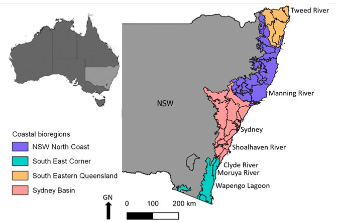
FIGURE 1. Location map showing the extent of the study region in New South Wales (NSW), Australia containing four costal bioregions. Estuary names referred to in the text are also shown.

The estuaries, and their adjacent land potentially subject to SLR inundation, display present-day land use that ranges from entirely natural to entirely modified by human activity and mixtures in between. The most common mangroves in NSW are Avicennia marina and Aegiceras corniculatum, which occur throughout the four NSW coastal bioregions (Figure 1). Other species such as Bruguiera gymnorhiza, Rhizophora stylosa and Excoecaria agallocha occur only in small stands, primarily in the South-eastern Queensland bioregion, with some scattered individuals in the northern part of the NSW North Coast bioregion (Duke 2006). The diversity of saltmarsh plants in NSW increases with increasing latitude (Saintilan, 2009). Common saltmarsh species in NSW include Baumea juncea, Ficinia nodosa, Juncus kraussii, Samolus repens, Sarcocornia quinqueflora, Selliera radicans, Sporobulus virginicus, Suaeda australis, Triglochin striata, and Zoysia macrantha (West et al., 1985; Adam et al., 1988; Saintilan, 2009).

3.2 Random Forest Modelling and Assessing Predicted Map Accuracy

3.2.1 Model Development and Implementation

The present-day distribution of mangrove and saltmarsh was modelled using the random forest (RF) algorithm implemented in the R package Caret (Kuhn, 2008). RF is a widely used supervised machine learning method for classification and regression (Oliveira et al., 2012), which has two useful features making it the preferred algorithm for many mapping applications (Vrieling et al., 2018). First, it is a non-parametric rule-based algorithm which makes no a priori assumptions about the relationship between the predictor variables and the response, and generally performs better than parametric methods for complex systems (Breiman, 2001). Second, it can deal with non-linearity and interactions among predictors better than generalised linear and additive models (Oliveira et al., 2012). A previous study undertaken in an estuary in the same region as this study found that RF was among the top classifiers for mapping wetlands in what is a heterogenous coastal environment (Wen and Hughes, 2020).

The dataset of random samples of co-located response and predictor variables was split into training (2/3) and testing (1/3) subsets using stratified random sampling. With the training dataset, the repeated (5 times) 10-fold cross-validation procedure was used for model tuning as it was a good balance for the bias-variance and accuracy-computation trade-offs. Repeated cross-validation gives many more out-of-sample datasets to compare, thus more precise assessments of how well the model performs. To be computationally efficient while optimising control over the model training process (Probst et al., 2019), a custom tuning grid approach was utilised to fine tune the two main hyper-parameters: 1) the number of variables that is randomly sampled at each split and 2) the number of trees in the forest (Kuhn, 2008). A two-dimensional search grid was manually specified for each RF-model with the first hyper-parameter ranging from 2 to 15 and the second having the values 500, 1000, and 1500 trees.

Using the tidal planes for each of the three SLR scenarios, the two hydrological variables h and d (Section 2.1.2) were recalculated for future sea levels. The trained and evaluated RF-models for predicting mangrove and saltmarsh distribution in the present-day landscape were then used to predict the future distribution of mangrove and saltmarsh for the landscape under each SLR scenario. To bracket the breadth of potential outcomes, and make the outcomes relevant for planning purposes, three sets of predictions were prepared for each SLR scenario. One where there was no restriction on future wetland location by existing land uses except urban land cover, and two where predictions of future wetland locations are excluded from areas currently under anthropogenically significant land use (e.g., urban, industrial, agricultural etc.), assuming that they might be partially or fully protected from present and future inundation. In the case where the predictions are limited by land use, one set of predictions are limited to protected lands such as reserves and natural conservation parks), and the other set additionally includes low intensity land uses such as grazed native vegetation.

3.2.2 RF-Model Predicted Map Accuracy Assessment

It is only possible to assess the accuracy of the model prediction for the present-day distribution of mangrove and saltmarsh. The reliability of the predictions under future SLR scenarios depends on the present-day model accuracy, and a range of unquantifiable processes in the future. The objective of our predicted map accuracy assessment was to provide robust estimates of the overall map accuracy and class-specific accuracy. We assessed the predicted present-day map accuracy through cell-by-cell comparison of the predicted mangrove, saltmarsh, background and water class distribution with the existing maps. Stratified random samples (50% of the grids) were created within the existing map, and the mapped and predicted classes were used to construct an error matrix.

The overall accuracy and the Kappa statistic are commonly provided metrics for map accuracy, but these can be confounded (Shao et al., 2019; Stehman and Foody, 2019), particularly if the class sizes are significantly unbalanced which is the case here. The F₁ score is commonly used to assess accuracy in the machine learning literature, but it is undesirably asymmetric and is independent of the number of samples correctly classified as negative (Chicco and Jurman, 2020). We therefore chose the Matthews correlation coefficient (MCC) to assess accuracy, which effectively balances Type I and Type II classification errors into a single statistic and is insensitive to unbalanced class sizes. Chicco and Jurman, (2020) provide a thorough analysis of the relative merits of the abovementioned metrics. MCC values are analogous to Pearson correlation coefficients (Chicco et al., 2021) and we use the following qualitative descriptors: 0.0–0.19 zero to negligible correlation, 0.2–0.39 weak correlation, 0.4–0.59 moderate correlation, 0.6–0.79 strong correlation, 0.8–1.0 very strong correlation (Evans, 1996).

4 Results

4.1 Regional Representativeness of the Outputs

The 184 significant estuaries in NSW include 9 coastal bays, 8 drowned river valleys, 21 riverine estuaries, 36 barrier (open entrance) estuaries, and 110 intermittently closed and open lakes and lagoons (Roper et al., 2011; Hughes et al., 2019). Only 110 of the 184 estuaries had sufficient areal extent of mangrove and/or saltmarsh to build an RF-model. In the case of riverine and barrier (open entrance) types 100% of these estuaries were modelled. Of the drowned river valleys, coastal bays and intermittently closed and open lakes and lagoons 88%, 56%, and 37%, respectively, were modelled. While the percentage of intermittently closed and open lakes and lagoons modelled was limited, mostly due to their small size and small wetland area, they are the most numerous estuary type so there was still a large number included. Overall, the range of estuary types and the estuaries with the largest areas of intertidal wetland (riverine, drowned river valley and barrier open entrance estuaries; Hughes et al., 2019) are well represented in the outputs.

4.2 Accuracy of the RF-Model Predictions

In many of the NSW estuaries anthropogenic land covers have modified the landscape to exclude saline wetlands all together. The most appropriate set of RF-model predictions to test against the present-day mapped distribution of mangrove and saltmarsh is therefore the model prediction constrained to natural land use covers. The MCC values for each estuary representing the correlation between predicted and mapped distribution of total wetland (mangrove and saltmarsh combined), or mangrove and saltmarsh separately are summarised in Figure 2A. The MCC values for total wetland were consistently high with a strong correlation or better (MCC>0.60) occurring in 65% of the modelled estuaries and a moderate correlation or better (MCC>0.40) occurring in 94% of them. The MCC values for mangrove and saltmarsh individually were not as strong. In the case of mangroves alone, a strong correlation or better occurred in 43% of the modelled estuaries containing mangrove and a moderate correlation or better occurred in 84% of them. For saltmarsh alone, a strong correlation or better occurred in 39% of the modelled estuaries containing saltmarsh and a moderate correlation or better occurred in 75% of them. The lower accuracy in predicting the present-day distribution of mangrove and saltmarsh individually, compared to predicting total wetland distribution, is largely because of model confusion between mangrove and saltmarsh. The MCC values for total wetland distribution, grouped by estuary type, are summarised in Figure 2B. The RF-models performed strongly in all the drowned river valley type estuaries, although, these represent a small component of the 110 estuaries modelled. Otherwise, the accuracy of the RF-models is reasonably similar across the estuary types. Figure 2C demonstrates no clear influence of total wetland area in the estuary on the RF-model performance for the estuary.

FIGURE 2

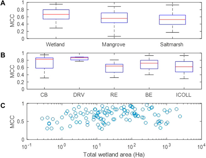
FIGURE 2. Boxplots of Matthews Correlation Coefficients (MCC) calculated from comparison between mapped wetland areas and predicted areas for present-day sea level and restricted natural land covers. The data set is grouped by (A) wetland type (wetland is mangrove plus saltmarsh combined), and (B) estuary type (CB—coastal bay, DRV—drowned river valley, RE—riverine estuary, BE—barrier estuary, ICOLL—intermittently closed, and open lake or lagoon). The median value is indicated by the horizontal red line, the lower and upper limit of the blue box are the 25th and 75th percentiles, and the dashed lines extend to the maximum and minimum value. (C) is the MCC value for total wetland (mangrove plus saltmarsh combined) plotted against total wetland area.

Comparison of the mapped versus predicted total wetland area, and mangrove and saltmarsh areas individually, for each of the 110 modelled estuaries is shown in Figure 3. The comparison demonstrates good overall correspondence, with a small to modest bias toward overpredicting wetland area. This overprediction is at least in part related to the fact that anthropogenic land uses in many catchments have resulted in removal of previously existing mangrove and saltmarsh areas, which the models are predicting should be there. Other relevant factors are discussed below (Section 5).

FIGURE 3

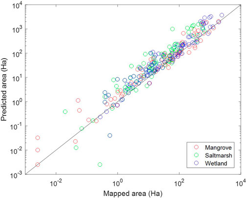
FIGURE 3. Mapped mangrove areas, saltmarsh areas, and total wetland areas (mangrove plus saltmarsh) versus predicted areas for each of the 110 estuaries. The black line is the 1:1 relationship.

Figure 4 shows the present-day mapped mangrove and saltmarsh areas compared to the RF-model prediction for an estuary where there is strong correlation and an estuary where there is only moderate correlation. Where there was strong correlation (cf. Figures 4A,B) large areas of mangrove and of saltmarsh were predicted in the correct locations and with the correct extents. Boundaries between mangrove and saltmarsh were also broadly correct. While there was minor confusion between mangrove and saltmarsh, confusion between either macrophyte and terrestrial background or open water areas was largely absent. Where there is only moderate correlation between mapped and RF-model prediction, there can be a variety of differences. In the example shown in Figures 4C,D the locations and extents of large areas of mangrove and saltmarsh are broadly correct. There is, however, significant confusion between mangrove and saltmarsh in the prediction leading to incorrect boundaries between the two. Furthermore, there is significant confusion between mangrove/saltmarsh and terrestrial in some areas resulting in the prediction of mangrove and saltmarsh where it does not occur. We recommend using predictions where MCC is between 0.4 and 0.6 with caution and predictions where MCC<0.4 should not be used.

FIGURE 4

FIGURE 4. Present-day mapped mangrove and saltmarsh areas (A) compared to model predictions for present day (B) for Wapengo Lagoon where the MCC values indicate very strong correlation—MCC is 0.91, 0.81, and 0.76 for total wetland, mangrove, and saltmarsh respectively. Present-day mapped mangrove and saltmarsh areas (C) compared to model predictions for present day (D) for Shoalhaven River where the MCC values indicate moderate correlation—MCC is 0.51, 0.41, and 0.33 for total wetland, mangrove, and saltmarsh respectively.

4.3 Relative Importance of Predictor Variables

The relative importance of predictor variables was evaluated for the RF-model determined for each of the 110 estuaries. To summarise the information, we have taken the relative importance for each predictor variable, grouped them by estuary type and calculated the mean and one standard deviation of each variable for each estuary type (Figure 5). While the relative importance of variables differed among estuary types, two predictors were ranked the most important for all RF-models—water depth at High High-Water Solstice Springs (h) and local deviation from a global window (LDFGW). The relative importance of other predictors varied among estuary types. For example, the importance of landscape surface texture (D) was larger than distance to water edge (d) for drowned river valley estuaries, but d was more important for all other estuaries. Generally, sediment type made the least contribution to model performance for all estuaries, but it was locally important in some estuaries and had higher importance than the compound topographic index (CTI) in intermittently closed and open lakes and lagoons (Figure 5).

FIGURE 5

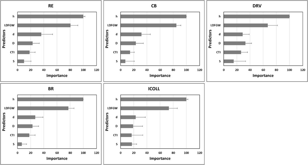
FIGURE 5. Charts summarising the importance of predictor variables in the RF models, scaled from 0 to 100 with the most important variable having the score 100. The mean importance (horizontal bar) and standard deviation (line) for each estuary type is shown. The notation for the predictors is defined in Table 1. The estuary types are riverine estuaries (RE), coastal bays (CB), drowned river valleys (DRV), barrier (open-entrance) estuaries (BR), and intermittently closed and open lakes and lagoons (ICOLLs). These estuary types are described in Section 3.1.

4.4 Illustrative Examples of Intertidal Wetland Migration Under Sea Level Rise

Overall, the MCC values suggest that the RF-models in most cases provide robust predictions for the distribution of intertidal wetlands in the present-day landscape across a variety of estuary types. This provides a level of confidence in applying the RF-models to predict the potential distribution of mangrove and saltmarsh in future landscapes under SLR scenarios. Some examples of predicted changes in mangrove and saltmarsh distribution under SLR are presented in Figures 6–8 to illustrate pertinent points for the discussion section.

FIGURE 6

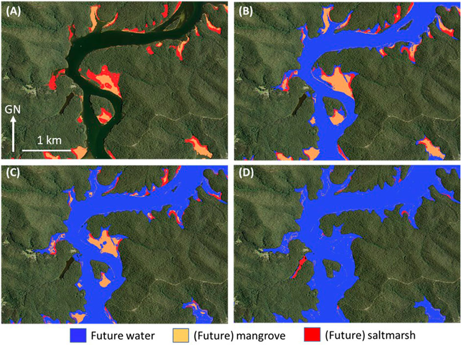
FIGURE 6. Area in the Clyde River (drowned river valley estuary type) showing distribution of mangrove and saltmarsh at (A) present-day; (B) 0.5 m SLR; (C) 1.0 m SLR; and (D) 1.5 m SLR. The future water area shown is that expected for high high-water solstice springs. The predictions are not influenced by land use since the area is entirely natural land covers. Images are oriented so that north is at the top.

A reach of the Clyde River estuary, a drowned river valley type estuary, with predominantly natural land-use, is shown in Figure 6. Following a 0.5 m SLR a modest increase in mangrove area is predicted at the expense of saltmarsh (cf. Figures 6A,B). Due to the steep supra-tidal topography there is limited lateral accommodation space, thus the present-day mangrove areas are shown migrating into present-day saltmarsh areas, with little opportunity for saltmarsh migration due to natural coastal squeeze. A 1.0 m SLR results in significant loss of the seaward margin of present-day mangrove areas due to excessive inundation and continued reduction in the saltmarsh areas as they are overtaken by mangrove (cf. Figures 6A,C). For the case of a 1.5 m SLR, virtually all mangrove and saltmarsh areas are gone due to excessive inundation and the naturally limited opportunities for migration have been exhausted (cf. Figures 6A,D).

A lower reach of the Tweed River estuary, a riverine type estuary, is shown in Figure 7. Comparing Figures 7A,B indicates that at present-day sea level there are some minor areas suitable for mangrove and saltmarsh that are currently excluded by residential development and related infrastructure (central areas present in Figure 7B and absent from Figure 7A). Under a 0.5 m SLR minor loss of mangrove at the seaward margins and significant encroachment of mangrove into previous saltmarsh areas is predicted (Figure 7C). Some predicted new opportunities for both mangrove and saltmarsh are identified under the same SLR scenario if existing land use constraints are relaxed (Figure 7D). Under a 1.5 m SLR all significant areas of wetland are predicted to be lost in this reach of the estuary due to excessive inundation and anthropogenic coastal squeeze (Figure 7E). If some anthropogenic land covers were given over to wetland migration several small areas of saltmarsh habitat are predicted to develop (Figure 7F).

FIGURE 7

FIGURE 7. Area in the lower Tweed River (riverine estuary type) showing predicted distribution of mangrove and saltmarsh at (A) present-day (restricted by land use); (B) present-day (no restriction); (C) 0.5 m SLR (restricted by land use); (D) 0.5 m SLR (no restriction); (E) 1.0 m SLR (restricted by land use); and (F) 1.0 m SLR (no restriction). The future water area shown is that expected for high high-water solstice springs. Images are oriented so that north is at the top.

A reach of the Moruya River, a riverine type estuary, is shown in Figure 8. At present-day sea level in this reach there are large wetland areas adjacent to low-lying floodplain dominated by pasture. There is relatively little difference between the present-day wetland area predictions under restricted versus unrestricted land-use scenarios (cf. Figures 8A,B). Under a 0.5 m SLR however, the saltmarsh areas to the north of the main east-west oriented river channel are predicted to be almost completely lost due to mangrove expansion (Figure 8C). Under the same 0.5 m SLR, if pasture is given up then there is the potential for a significant area of saltmarsh to be retained through migration into a newly inundated area (Figure 8D).

FIGURE 8

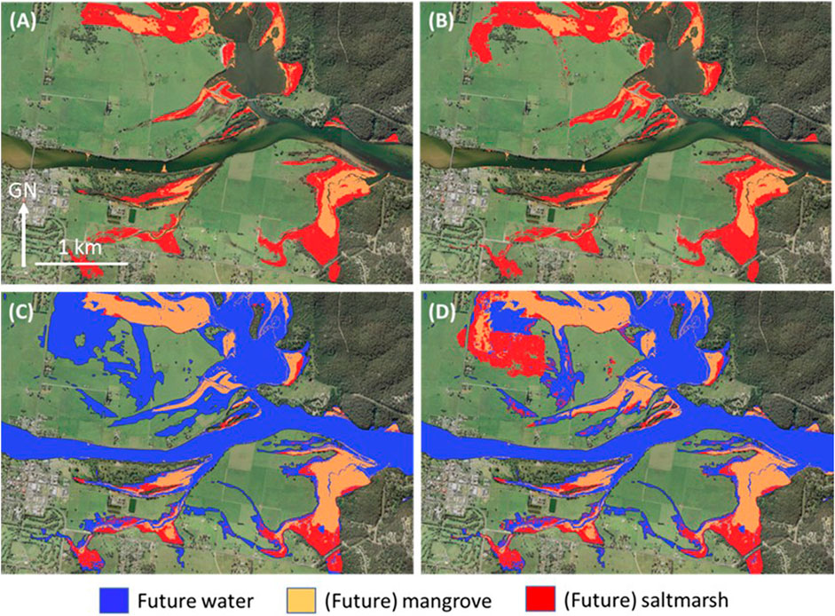
FIGURE 8. Area in the Moruya River (riverine estuary type) showing predicted distribution of mangrove and saltmarsh at (A) present-day (restricted by land use); (B) present-day (no restriction); (C) 0.5 m SLR (restricted by land use); and (D) 0.5 m SLR (no restriction). The future water area shown is that expected for high high-water solstice springs. Images are oriented so that north is at the top.

5 Discussion

We have developed and demonstrated a classification method to predict mangrove and saltmarsh distribution in the landscape at regional scale. The method is demonstrably robust in predicting present-day saline wetland distribution, with moderate correlation or better between predicted and mapped distribution occurring in nearly all estuaries and strong correlation or better occurring in more than half of the estuaries. When combined with the latest intra-estuary SLR modelling the classification method has reproduced several previously documented regional aspects of wetland response to SLR and coastal development. Wetland exclusion from suitable areas in the present-day landscape by coastal infrastructure and development (e.g., Stricker, 1995; Ross and Adam, 2013) was illustrated in the Tweed River estuary (Figure 7). Mangrove dieback along the seaward margins due to excessive inundation (e.g., Adams and Human, 2016) under SLR was illustrated in the Clyde River and Tweed River estuaries (Figures 6, 7). Mangrove migration into saltmarsh areas (e.g., Saintilan and Williams, 2000) was demonstrated as an important process beginning with the smallest SLR scenario in the Clyde, Tweed and Moruya River estuaries (Figures 6–8). Finally, coastal squeeze (e.g., Borchert et al., 2018) due to natural topography was demonstrated in the Clyde River estuary with almost complete loss of saltmarsh, due to mangrove migration into saltmarsh areas and no accommodation space upslope for saltmarsh to migrate into (Figure 6). Similarly, coastal squeeze due to coastal development was demonstrated in the Tweed River estuary (urban) and Moruya River estuary (agricultural). These latter two cases provide examples of how changes in land use zoning under future sea levels offer potential opportunities for increasing wetland area and reducing vulnerability. The opportunities are likely to be greater in agricultural rather than urban areas.

One hydrological and one topographic variable were the two most important predictors in the RF-Models for all estuary types (Figure 5). NSW mangroves and saltmarshes are associated with locally distinct tidal inundation regimes (Hughes et al., 2019; Kumbier et al., 2021), thus the hydrological variable, h (i.e., water depth at HHWSS), was the most important predictor variable since it is the surrogate for tidal inundation regime. The topographic variable, LDFGW (i.e., the local deviation from global window) is an indicator of the local smoothness and convexity/concavity of the land surface. LDFGW has also emerged as an important predictor for vegetation in other wetland studies (Powell et al., 2019; Shaeri Karimi et al., 2019; Wen and Hughes, 2020), where values indicate approximately planar (and shallow basin) topography, with horizontal to gently dipping surfaces that receive overland flow and are poorly drained. The pattern of importance in the minor predictor variables was generally consistent across the five estuary types, except that the topographical variable D (dissection) was marginally more important in Drowned River Valley estuaries (Figure 5). This is possibly due to a greater prevalence of tidal creeks and large variations in elevation across small distances at the margins of wetlands in these estuaries, associated with the steep up-slope topography.

The RF-models applied to present-day conditions performed robustly with respect to predicting total wetland distribution and distributions of mangroves or saltmarsh individually, although the accuracy was generally lower in the latter case. Furthermore, in many estuaries there was a small to modest overprediction in the wetland areas. There are several factors contributing to errors in prediction. Misclassification between the mangrove and saltmarsh classes, due to the subtle differences in topographic and hydrologic predicters between the two being close to the resolution limits of the DEM and tidal plane layers was one source. In some cases, overprediction of wetland areas arose from predicted areas being disconnected from tidal inundation due to the presence of structures or other landscape modification, or potential fresh groundwater input. This affected saltmarsh more than mangrove due to its more elevated position in the landscape. Use of the classified land cover map to exclude such areas was partially successful, however, the best mix of land covers to exclude seemed to vary between estuary type. Some improvement in predictive accuracy could be achieved by optimising the choice of land covers to exclude on an estuary by estuary basis and by compiling a data base of tidal gates and other flow restricting structures. In several estuaries the wetlands appear as numerous relatively small isolated areas amongst large areas of background. This means there is potential for true background areas to be sufficiently close to being suitable for wetlands and thus falsely classified as such. Finally, potential errors in all the foundational data layers, particularly the DEM and macrophyte mapping, influenced predictive accuracy. None of these factors can be readily resolved without obtaining higher resolution data and/or obtaining more site-specific information from each estuary, which is beyond the scope of regional-scale applications.

5.1 Broader Application of the Method

Maps of potential future mangrove and saltmarsh distribution developed using the method described here could be used in regional-scale assessments of intertidal wetland vulnerability to sea level rise, either as a factor on their own or combined with other information. For example, predicted losses and gains in intertidal wetland area between present day and future sea level scenarios can be calculated and used as a first-pass means of assessing vulnerability. Moreover, the opportunities arising from land use planning to accommodate intertidal wetland migration to new areas can be assessed by comparing maps for present day wetland distribution with predicted future distributions constrained by present-day land use covers, and with future distributions that are unconstrained.

Predicting areas in the landscape that are potentially suited to intertidal wetland under future sea level scenarios as described herein addresses only one of the likely responses of intertidal wetlands to sea level rise, i.e., horizontal migration. Some wetlands may accumulate sediment and vegetation may grow at a sufficient rate to keep up with sea level rise and thus maintain their present-day position in the landscape (e.g., Woodroffe and Davies, 2009; Rogers et al., 2019). Climatic drivers may change the latitudinal range of vegetation species and consequently the wetland type entirely (e.g., Osland et al., 2016). The method and corresponding outputs presented here are also suited to being incorporated with information addressing these other factors, which would be included in a comprehensive intertidal wetland vulnerability assessment.

6 Conclusion

We have demonstrated a novel method for predicting the potential distribution of intertidal wetlands (mangrove and saltmarsh) in the present-day landscape and future landscapes under specified sea level scenarios. The method is demonstrably robust in predicting the present-day distribution of intertidal wetlands and is therefore assumed to be informative in predicting potential future distributions when combined with the best available intra-estuary tidal plane models of SLR. The method reproduces several previously documented regional aspects of wetland response to SLR and coastal development, including wetland exclusion from suitable areas in the present-day landscape by coastal infrastructure and development, mangrove dieback due to excessive inundation, mangrove migration into saltmarsh areas and coastal squeeze.

The method utilises a variety of hydro-geomorphological surrogates that can be derived from digital elevation models, Quaternary geology or soils mapping, land use mapping and a representation of the future sea level inside estuaries. Here we used projected tidal planes inside estuaries under future ocean sea level scenarios. A bath-tub approach to future sea level inside the estuary might also be applied but would be less accurate. Application of the method at the regional scale has been demonstrated for NSW, Australia, which contains 184 estuaries including five different estuary types distributed along nearly 2,000 km of coastline. It is anticipated that outputs from applying the method there and elsewhere would inform assessments of intertidal wetland vulnerability to SLR and guide planning for potential wetland migration pathways.

Data Availability Statement

The raw data supporting the conclusions of this article will be made available by the authors, without undue reservation.

Author Contributions

MH, LW and TG designed the overall study and method. LW undertook the geospatial analysis. TG and GW contributed detailed knowledge of the macrophyte maps dataset. DH contributed detailed knowledge of the intra-estuary tidal planes and SLR datatset. MH analysed the results with aid from all authors. All authors provided critical feedback and helped shape the research, analysis, and manuscript.

Funding

This work was funded by the New South Wales Government via the NSW Marine Estate Management Strategy.

Conflict of Interest

The authors declare that the research was conducted in the absence of any commercial or financial relationships that could be construed as a potential conflict of interest.

Publisher’s Note

All claims expressed in this article are solely those of the authors and do not necessarily represent those of their affiliated organizations, or those of the publisher, the editors and the reviewers. Any product that may be evaluated in this article, or claim that may be made by its manufacturer, is not guaranteed or endorsed by the publisher.

Acknowledgments

The authors acknowledge and thank Brad Morris for reprocessing the existing sea level rise tidal plane spatial data layers to make them suitable for use in this study.

References

Adam, P. (2009). “Australian Saltmarshes in Global Context,” in Australian Saltmarsh Ecology. Editor N. Saintilan (Melbourne: CSIRO Publishing).

Google Scholar

Adam, P. (1978). Geographical Variation in British Saltmarsh Vegetation. J. Ecol. 66, 339–366. doi:10.2307/2259141

CrossRef Full Text | Google Scholar

Adam, P., Wilson, N. C., and Huntley, B. (1988). The Phytosociology of Coastal Saltmarsh Vegetation in New South Wales. Wetl. Aust. 7, 35–85. doi:10.31646/wa.111

CrossRef Full Text | Google Scholar

Adams, J. B., and Human, L. R. D. (2016). Investigation into the Mortality of Mangroves at St. Lucia Estuary. South Afr. J. Bot. 107, 121–128. doi:10.1016/j.sajb.2016.03.018

CrossRef Full Text | Google Scholar

Barbier, E. B., Hacker, S. D., Kennedy, C., Koch, E. W., Stier, A. C., and Silliman, B. R. (2011). The Value of Estuarine and Coastal Ecosystem Services. Ecol. Monogr. 81, 169–193. doi:10.1890/10-1510.1

CrossRef Full Text | Google Scholar

Borchert, S. M., Osland, M. J., Enwright, N. M., Griffith, K. T., and Rohr, J. (2018). Coastal Wetland Adaptation to Sea Level Rise: Quantifying Potential for Landward Migration and Coastal Squeeze. J. Appl. Ecol. 55, 2876–2887. doi:10.1111/1365-2664.13169

CrossRef Full Text | Google Scholar

Breiman, L. (2001). Random Forests. Mach. Learn. 45, 5–32. doi:10.1023/a:1010933404324

CrossRef Full Text | Google Scholar

Chicco, D., and Jurman, G. (2020). The Advantages of the Matthews Correlation Coefficient (MCC) Over F1 Score and Accuracy in Binary Classification Evaluation. BMC Genomics 21. doi:10.1186/s12864-019-6413-7

PubMed Abstract | CrossRef Full Text | Google Scholar

Chicco, D., Tötsch, N., and Jurman, G. (2021). The Matthews Correlation Coefficient (MCC) Is More Reliable Than Balanced Accuracy, Bookmaker Informedness, and Markedness in Two-Class Confusion Matrix Evaluation. BioData Min. 14. doi:10.1186/s13040-021-00244-z

CrossRef Full Text | Google Scholar

Corcoran, J., Knight, J., and Gallant, A. (2013). Influence of Multi-Source and Multi-Temporal Remotely Sensed and Ancillary Data on the Accuracy of Random Forest Classification of Wetlands in Northern Minnesota. Remote Sens. 5, 3212–3238. doi:10.3390/rs5073212

CrossRef Full Text | Google Scholar

Doughty, C. L., Cavanaugh, K. C., Ambrose, R. F., and Stein, E. D. (2018). Evaluating Regional Resiliency of Coastal Wetlands to Sea Level Rise Through Hypsometry‐Based Modeling. Glob. Change Biol. 25, 78–92. doi:10.1111/gcb.14429

CrossRef Full Text | Google Scholar

Dubeau, P., King, D., Unbushe, D., and Rebelo, L.-M. (2017). Mapping the Dabus Wetlands, Ethiopia, Using Random Forest Classification of Landsat, PALSAR and Topographic Data. Remote Sens. 9, 1056. doi:10.3390/rs9101056

CrossRef Full Text | Google Scholar

Duke, N. (2006). Australia's Mangroves: An Authoritative Guide to Australia’s Mangrove Plants. Brisbane, QLD, Australia: University of Queensland.

Google Scholar

Evans, J. D. (1996). Straightforward Statistics for the Behavioural Sciences. Pacific Grove: Brooks/Cole Publishing.

Google Scholar

Felton, B. R., O’Neil, G. L., Robertson, M.-M., Fitch, G. M., and Goodall, J. L. (2019). Using Random Forest Classification and Nationally Available Geospatial Data to Screen for Wetlands Over Large Geographic Regions. Water 11, 1158. doi:10.3390/w11061158

CrossRef Full Text | Google Scholar

Gabler, C. A., Osland, M. J., Grace, J. B., Stagg, C. L., Day, R. H., Hartley, S. B., et al. (2017). Macroclimatic Change Expected to Transform Coastal Wetland Ecosystems This Century. Nat. Clim. Change 7, 142–147. doi:10.1038/nclimate3203

CrossRef Full Text | Google Scholar

Galloway, R. W. (1982). “Distribution and Physiographic Patterns of Australian Mangroves,” in Mangrove Ecosystems in Australia: Structure, Function and Management. Editor B. F. Clough, 31–54.

Google Scholar

Geoscience Australia (2021). Border Lengths – States and Territories. Available at: https://www.ga.gov.au/scientific-topics/national-location-information/dimensions/border-lengths (Accessed July 29, 2021).

Google Scholar

Hanslow, D. J., Morris, B. D., Foulsham, E., and Kinsela, M. A. (2018). A Regional Scale Approach to Assessing Current and Potential Future Exposure to Tidal Inundation in Different Types of Estuaries. Sci. Rep. 8, 7065. doi:10.1038/s41598-018-25410-y

PubMed Abstract | CrossRef Full Text | Google Scholar

Hughes, M. G., Roger, K., and Wen, L. (2019). Saline Wetland Extents and Tidal Inundation Regimes on a Micro-Tidal Coast, New South Wales, Australia. Coast. Shelf Sci. 227. doi:10.1016/j.ecss.2019.106297

CrossRef Full Text | Google Scholar

Khojasteh, D., Hottinger, S., Felder, S., De Cesare, G., Heimhuber, V., Hanslow, D. J., et al. (2020). Estuarine Tidal Response to Sea Level Rise: The Significance of Entrance Restriction. Estuar. Coast. Shelf Sci. 244, 106941. doi:10.1016/j.ecss.2020.106941

CrossRef Full Text | Google Scholar

Kirwan, M. L., and Megonigal, J. P. (2013). Tidal Wetland Stability in the Face of Human Impacts and Sea-Level Rise. Nature 504, 53–60. doi:10.1038/nature12856

PubMed Abstract | CrossRef Full Text | Google Scholar

Kuhn, M. (2008). Building Predictive Models in R Using the Caret Package. J. Stat. Softw. 28, 1–26. doi:10.18637/jss.v028.i05

PubMed Abstract | CrossRef Full Text | Google Scholar

Kumbier, K., Hughes, M. G., Rogers, K., and Woodroffe, C. D. (2021). Inundation Characteristics of Mangrove and Saltmarsh in Micro-Tidal Estuaries. Estuar. Coast. Shelf Sci. 261, 107553. doi:10.1016/j.ecss.2021.107553

CrossRef Full Text | Google Scholar

Mahdianpari, M., Salehi, B., Mohammadimanesh, F., and Motagh, M. (2017). Random Forest Wetland Classification Using ALOS-2 L-Band, RADARSAT-2 C-Band, and TerraSAR-X Imagery. ISPRS J. Photogrammetry Remote Sens. 130, 13–31. doi:10.1016/j.isprsjprs.2017.05.010

CrossRef Full Text | Google Scholar

Manly Hydraulics Laboratory (2012). OEH NSW Tidal Planes Analysis: 1990-2010 Harmonic Analysis. Report MHL2053. Sydney: NSW Public Works.

Google Scholar

Molino, G. D., Defne, Z., Aretxabaleta, A. L., Ganju, N. K., and Carr, J. A. (2021). Quantifying Slopes as a Driver of Forest to Marsh Conversion Using Geospatial Techniques: Application to Chesapeake Bay Coastal-Plain, United States. Front. Environ. Sci. 9. doi:10.3389/fenvs.2021.616319

CrossRef Full Text | Google Scholar

Moore, I. D., Grayson, R. B., and Ladson, A. R. (1991). Digital Terrain Modelling: A Review of Hydrological, Geomorphological, and Biological Applications. Hydrol. Process. 5, 3–30. doi:10.1002/hyp.3360050103

CrossRef Full Text | Google Scholar

Morris, J. T., Sundareshwar, P. V., Nietch, C. T., Kjerfve, B., and Cahoon, D. R. (2002). Responses of Coastal Wetlands to Rising Sea Level. Ecology 83, 2869–2877. doi:10.1890/0012-9658(2002)083[2869:rocwtr]2.0.co;2

CrossRef Full Text | Google Scholar

Mutanga, O., Adam, E., and Cho, M. A. (2012). High Density Biomass Estimation for Wetland Vegetation Using WorldView-2 Imagery and Random Forest Regression Algorithm. Int. J. Appl. Earth Observation Geoinformation 18, 399–406. doi:10.1016/j.jag.2012.03.012

CrossRef Full Text | Google Scholar

Oliveira, S., Oehler, F., San-Miguel-Ayanz, J., Camia, A., and Pereira, J. M. C. (2012). Modeling Spatial Patterns of Fire Occurrence in Mediterranean Europe Using Multiple Regression and Random Forest. For. Ecol. Manag. 275, 117–129. doi:10.1016/j.foreco.2012.03.003

CrossRef Full Text | Google Scholar

Osland, M. J., Enwright, N. M., Day, R. H., Gabler, C. A., Stagg, C. L., and Grace, J. B. (2016). Beyond Just Sea‐Level Rise: Considering Macroclimatic Drivers Within Coastal Wetland Vulnerability Assessments to Climate Change. Glob. Change Biol. 22, 1–11. doi:10.1111/gcb.13084

CrossRef Full Text | Google Scholar

Powell, M., Hodgins, G., Danaher, T., Ling, J., Hughes, M., and Wen, L. (2019). Mapping Wetland Types in Semiarid Floodplains: A Statistical Learning Approach. Remote Sens. 11 (6), 609. doi:10.3390/rs11060609

CrossRef Full Text | Google Scholar

Probst, P., Boulesteix, A. L., and Bischl, B. (2019). Tunability: Importance of Hyperparameters of Machine Learning Algorithms. J. Mach. Learn. Res. 20 (1), 1934–1965.

Google Scholar

Raposa, K. B., Wasson, K., Smith, E., Crooks, J. A., Delgado, P., Fernald, S. H., et al. (2016). Assessing Tidal Marsh Resilience to Sea-Level Rise at Broad Geographic Scales with Multi-Metric Indices. Biol. Conserv. 204, 263–275. doi:10.1016/j.biocon.2016.10.015

CrossRef Full Text | Google Scholar

Rogers, K., Boon, P. I., Branigan, S., Duke, N. C., Field, C. D., Fitzsimons, J. A., et al. (2016). The State of Legislation and Policy Protecting Australia's Mangrove and Salt Marsh and Their Ecosystem Services. Mar. Policy 72, 139–155. doi:10.1016/j.marpol.2016.06.025

CrossRef Full Text | Google Scholar

Rogers, K., Kelleway, J. J., Saintilan, N., Megonigal, J. P., Adams, J. B., Holmquist, J. R., et al. (2019). Wetland Carbon Storage Controlled by Millennial-Scale Variation in Relative Sea-Level Rise. Nature 567, 91–95. doi:10.1038/s41586-019-0951-7

PubMed Abstract | CrossRef Full Text | Google Scholar

Roper, T., Creese, B., Scanes, P., Stephens, K., Williams, R., Dela-Cruz, J., et al. (2011). Assessing the Condition of Estuaries and Coastal Lake Ecosystems in NSW. Sydney: NSW Office of Environment and Heritage.

Google Scholar

Ross, P., and Adam, P. (2013). Climate Change and Intertidal Wetlands. Biology 2, 445–480. doi:10.3390/biology2010445

PubMed Abstract | CrossRef Full Text | Google Scholar

Roy, P. S., Williams, R. J., Jones, A. R., Yassini, I., Gibbs, P. J., Coates, B., et al. (2001). Structure and Function of South-East Australian Estuaries. Estuar. Coast. Shelf Sci. 53, 351–384. doi:10.1006/ecss.2001.0796

CrossRef Full Text | Google Scholar

Saintilan, N. (2009). Biogeography of Australian Saltmarsh Plants. Austral Ecol. 34, 929–937. doi:10.1111/j.1442-9993.2009.02001.x

CrossRef Full Text | Google Scholar

Saintilan, N., and Williams, R. J. (2000). The Decline of Saltmarsh in Southeast Australia: Results of Recent Surveys. Wetl. Aust. 18, 49–54. doi:10.31646/wa.228

CrossRef Full Text | Google Scholar

Schuerch, M., Spencer, T., Temmerman, S., Kirwan, M. L., Wolff, C., Lincke, D., et al. (2018). Future Response of Global Coastal Wetlands to Sea-Level Rise. Nature 561, 231–234. doi:10.1038/s41586-018-0476-5

PubMed Abstract | CrossRef Full Text | Google Scholar

Shaeri Karimi, S., Saintilan, N., Wen, L., and Valavi, R. (2019). Application of Machine Learning to Model Wetland Inundation Patterns Across a Large Semiarid Floodplain. Water Resour. Res. 55 (11), 8765–8778. doi:10.1029/2019WR024884

CrossRef Full Text | Google Scholar

Shao, G., Tang, L., and Liao, J. (2019). Overselling Overall Map Accuracy Misinforms About Research Reliability. Landsc. Ecol. 34, 2487–2492. doi:10.1007/s10980-019-00916-6

CrossRef Full Text | Google Scholar

Spencer, T., Schuerch, M., Nicholls, R. J., Hinkel, J., Lincke, D., Vafeidis, A. T., et al. (2016). Global Coastal Wetland Change Under Sea-Level Rise and Related Stresses: The DIVA Wetland Change Model. Glob. Planet. Change 139, 15–30. doi:10.1016/j.gloplacha.2015.12.018

CrossRef Full Text | Google Scholar

Stehman, S. V., and Foody, G. M. (2019). Key Issues in Rigorous Accuracy Assessment of Land Cover Products. Remote Sens. Environ. 231, 111199. doi:10.1016/j.rse.2019.05.018

CrossRef Full Text | Google Scholar

Stricker, J. (1995). Reviving Wetlands. Wetl. Aust. 14, 20–25. doi:10.31646/wa.174

CrossRef Full Text | Google Scholar

Townend, I., and Pethick, J. (2002). Estuarine Flooding and Managed Retreat. Philo. Trans. R. Soc. Lond. Ser. A Math. Physi. Eng. Sci. 360, 1477–1495. doi:10.1098/rsta.2002.1011

PubMed Abstract | CrossRef Full Text | Google Scholar

Troedson, A. (2015). Coastal Quaternary Geology Mapping: Southern Hunter to Northern Illawarra, NSW. Report GS2015/1188. Maitland: Geological Survey of New South Wales.

Google Scholar

Vrieling, A., Meroni, M., Darvishzadeh, R., Skidmore, A. K., Wang, T., Zurita-Milla, R., et al. (2018). Vegetation Phenology from Sentinel-2 and Field Cameras for a Dutch Barrier Island. Remote Sens. Environ. 215, 517–529. doi:10.1016/j.rse.2018.03.014

CrossRef Full Text | Google Scholar

Wen, L., and Hughes, M. (2020). Coastal Wetland Mapping Using Ensemble Learning Algorithms: A Comparative Study of Bagging, Boosting and Stacking Techniques. Remote Sens. 12, 1683. doi:10.3390/rs12101683

CrossRef Full Text | Google Scholar

West, R. J., Thorogood, C., Walford, T., and Williams, R. J. (1985). An Estuarine Inventory for New South Wales, Australia. Fisheries Bulletin, 2. NSW, Australia: Department of Agriculture.

Google Scholar

Woodroffe, C. D., and Davies, G. (2009). “The Morphology and Development of Tropical Coastal Wetlands,” in Coastal Wetlands: An Integrated Ecosystem Approach. Editors G. Perillo, E. Wolanski, D. Cahoon, and M. Brinson (Amsterdam: Elsevier).

Google Scholar