Prediction of groundwater pollution diffusion path based on multi-source data fusion

In order to improve the prediction accuracy of groundwater pollution diffusion path, this paper combines multivariate data fusion technology to predict and analyze the groundwater pollution diffusion path. Under the special two-strategy swarm game model of water pollution particle swarm, this paper introduces replication dynamics with bounded continuous time-delay. Moreover, considering the dynamic behavior in both cases of constant kernel function and exponential kernel function, the hawk-dove game model is a special case of the model we are discussing. In addition, this paper proposes a method combining leaching surface and flux concentration, and applies numerical simulation method to simulate and analyze transient leakage monitoring of similar point and line source pollution in planar two-dimensional heterogeneous aquifers. The experimental study verifies that the multivariate data fusion proposed in this paper can play an important role in the prediction of groundwater pollution diffusion path.

Introduction

Due to the complex formation of underground strata and extremely slow groundwater flow, groundwater pollution is characterized by slow process, difficult to find and difficult to manage. In particular, it is concealed and delayed in the early stage, and when it is found that the water quality has changed significantly, it has been polluted or seriously polluted (Bakhoum et al., 2020). Due to the continuous migration and circulation of groundwater, through runoff, discharge, water supply and other means, in the complex geological environment system, the groundwater system is closely hydraulically linked. Once groundwater is polluted, it is difficult to determine the scope of pollution and to restore it. Even if pollution and pollution sources are completely eliminated, it will take decades or even decades to restore water quality (Chao et al., 2020).

Sudden water pollution is very contingent and instantaneous, and a large amount of toxic and harmful pollutants are suddenly leaked in a relatively short period of time, which poses a great threat to the safety of water sources, and has high requirements for the timeliness of treatment and disposal., it is very difficult to deal with (Pandiarajan et al., 2019). Groundwater quality evaluation can quantitatively describe the pros and cons of groundwater environment. So far, twenty or thirty water quality evaluation methods have been widely used in the field of water environment (Rathi, 2021), such as single factor evaluation method, comprehensive index method, fuzzy mathematics method, etc. Literature (Ballen et al., 2021) used single factor evaluation method and fuzzy mathematics method to evaluate groundwater quality. Using the concept of section capacity, the water quality evaluation method was optimized to evaluate the water quality under different hydrological conditions. However, the usual water quality evaluation methods can only evaluate the excessive components and water quality grades of groundwater, and cannot determine the source of the excessive components in groundwater. Many scientific researchers have applied a variety of different methods to determine the source of groundwater pollution. Literature (Tshamala et al., 2021) applied genetic algorithm to the identification of groundwater pollution sources, and used a small amount of pollutant monitoring data to identify the source of groundwater pollution in regional sites. Literature (Santonastaso et al., 2021) established a simulation-optimization method and applied it to a polluted site. This method can use a small amount of pollutant data to deduce the amount of pollutants released by the pollution source at different times, so as to identify the groundwater of the site. Source of pollution. In the established pollution source identification index system, literature (MabvounaBiguioh et al., 2020) summarized and explored the key factors of groundwater pollution sources such as priority control of pollutants and pollution source characteristics, and used the means derived from the hazard level in the identification of groundwater pollution sources. Literature (Jongman et al., 2020) believes that the main method to identify the sources of trinitrogen pollution in groundwater is the combination of stable isotope tracing method and various identification methods. The existing exploration methods can effectively identify the sources of trinitrogen pollution in groundwater, but various pollution sources are not effective in identifying the sources of trinitrogen pollution in groundwater. The contribution ratio of three nitrogen pollution sources is not accurate and still needs to be improved. Literature (Bayat et al., 2021) used factor analysis in multivariate statistical methods to determine the source of groundwater pollution. Comparing the various pollution source identification methods mentioned above and the factor analysis method in the multivariate statistical method, by analyzing the relationship between the observed factors, the complex and multiple variables can be summarized into a small number of comprehensive factors, eliminating unnecessary factors. Intervention information to find out the main factors that lead to the deterioration of groundwater quality and their relative pollution sources does not require high continuity of the original water quality data, so this factor analysis method is often used in the identification of groundwater pollution sources.

Risk represents the probability of a certain damage or loss occurring in a certain period of time under a certain environment, and is composed of risk. Risk. Factor, risk. Receptor, risk. Accident, risk. Loss. Although a unified evaluation system for groundwater pollution risk has not yet been formed, after continuous exploration by domestic and foreign researchers, its concept has increasingly become scientific, comprehensive, and systematic (Motlagh and Yang, 2019). Literature (Kitajima et al., 2018) pointed out that the risk of groundwater pollution is the probability that groundwater is polluted under the action of human activities to reach its maximum acceptable pollution level, which is the result of the vulnerability of groundwater and the pollutants produced by human activities. Literature (Song et al., 2021) defines the risk of groundwater pollution as the possibility of occurrence of events that are caused by natural geological factors or human activities, but use groundwater as a medium for its circulation, thereby having a malignant impact on human health and the environment. Literature (Peng et al., 2021) used the mathematical expectation of groundwater pollution to express pollution risk. Literature (Tripathi and Chaurasia, 2020) used the DRASTIC model to evaluate the vulnerability of groundwater in the plain river network area (Shanghai), and then evaluated the risk of groundwater pollution in this area. Based on the DRASTIC-GIS model, the vulnerability of groundwater in typical regions was evaluated. Literature (Domańska et al., 2019) used the DRASTIC model and HYDRUS-1D and the MODFLOW simulation block of GMS to evaluate groundwater pollution risk. Literature (Bezagio et al., 2020) proposes a pollution risk assessment method for groundwater protection by realizing the visualization of solute transport model simulation, which can predict the pollution level and transport distance of specific pollutants in a site. Literature (Cope et al., 2019) used Hydrus-1D and VisualModflow to simulate the subsurface flow zone process and the saturated zone process simulation, respectively, and formulated their own pollution warning thresholds for the subsurface layer and the confining layer. The vulnerability of the aquifer to contamination was assessed and validated by applying hydrogeological and hydrothermal chemical methods, and the groundwater vulnerability of the site was mapped using the DRASTIC model. Literature (Kaushik et al., 2018) proposed a groundwater pollution risk assessment method with the objective of protecting the civil well, and used this method to conduct groundwater pollution risk assessment in a simple landfill. According to the inherent stochastic property of groundwater, a groundwater pollution risk assessment method based on uncertainty process simulation is summarized.

The migration and transformation process in groundwater is simulated and predicted that pollutants entering groundwater must pass through the vadose zone. Factors such as the lithology of the vadose zone and the height of the vadose zone can directly affect the pollution source intensity of the pollutants entering the groundwater. The more mature software for the transformation of pollutants in the vadose zone is HYDRUS-1D (Fereidooni et al., 2021). The HYDRUS-1D model (Zhang et al., 2018) can simulate groundwater moisture transport, thermal transport and the transport of various solutes. This model summarizes water transport, solute transport and crop root absorption, and is applicable to various boundary conditions such as atmospheric boundary and constant water head boundary. At present, the HYDRUS model has been widely used in many aspects such as nitrogen migration and water resource evaluation at home and abroad.

This paper combines the multivariate data fusion technology to predict and analyze the groundwater pollution diffusion path to improve the prediction accuracy of the groundwater pollution diffusion path.

Stability of replication dynamics with bounded continuously distributed delays

Model description and derivation

The concept of the evolutionary stable state of the water pollution particle swarm game is given. At the same time, the replication dynamics model with bounded continuous distribution time delay is deduced in detail under a special kind of game model of single water pollution particle swarm of two-strategy water pollution particle swarm.

Definition 1. PG=(X, F) is a single water pollution particle swarm game. If the social state $\overline{x}\in X$ satisfies the following conditions:

(1)$\overline{x}$ is the Nash equilibrium of the single water pollution particle swarm game PG.

(2)There is a neighborhood $U_{\overline{x}}$ of $\overline{x}$ such that for any $\in U_{\overline{x}}$ , there is:

$〈y-\overline{x},F\left(\overline{x}\right)〉=0\Rightarrow 〈y-\overline{x},F\left(y\right)〉<0.(1)$

Then, the social state $\overline{x}$ is called the evolutionary stable state (ESS) of the single-water pollution particle swarm game PG.

Note 1. It can be seen from the above definition that the evolutionary stable state is actually a refinement of the Nash equilibrium, in which the first condition is the equilibrium condition and the second condition is the stability condition. It should be noted that although the ESS is still a static concept, condition 2) already reflects the dynamic idea. If social state y is the optimal response of $\overline{x}$ , condition 2) means that when social state changes to y, social state $\overline{x}$ is better than y.

The legacy is that not all water pollution particle swarm games have evolutionary stable states.

Example 1. PG is a water pollution particle swarm game model with three strategies of single water pollution particle swarm. Therefore, the social state space is $=\left\{\left(x_1,x_2,x_3\right)\in {\mathbb{R}}_{+}|x_1+x_2+x_3=1\right\}$ . For any social state $\in X$ , the payoff function $F:X\to {\mathbb{R}}^3$ of the water pollution particle swarm game PG is defined as:

$F\left(x\right)=\left(\begin{array}{c}{F}_1\left(x\right)\\ F_2\left(x\right)\\ F_2\left(x\right)\end{array}\right)=\left(\begin{array}{c}{x}_1+2x_2\\ x_2+2x_3\\ 2x_1+x_3\end{array}\right)$

It is easy to verify that the social state $x=\left(\frac{1}{3},\frac{1}{3},\frac{1}{3}\right)$ is the only Nash equilibrium of PG by the definition of Nash equilibrium in the water pollution particle swarm game. In the following, we show that condition 2) in Definition 1 does not hold.

In fact, for any social state $=\left(y_1,y_2,y_3\right)\in X$ , it is easy to see that:

$\begin{array}{l}〈y-\overline{x},F\left(\overline{x}\right)〉=〈\left(y_1-\frac{1}{3},y_2-\frac{1}{3},y_3-\frac{1}{3}\right),\left(\mathrm{1,1,1}\right)〉\\ =y_1+y_2+y_3-1\\ =0\end{array}$

If we take $y=\left(y_1,y_2,y_3\right)=\left(\mathrm{1,0,0}\right)$, then there is F(y)=(1,0,2), thus

$\begin{array}{l}〈y-\overline{x},F\left(y\right)〉=〈\left(y_1-\frac{1}{3},y_2-\frac{1}{3},y_3-\frac{1}{3}\right),\left(\mathrm{1,0,2}\right)〉\\ =0\nless 0.\end{array}$

Therefore, condition 2) in Definition 1 cannot be established.

We assume that there is a water pollution particle swarm composed of a sufficiently large number of individuals, in which the individuals repeatedly interact with each other through random matching. In each strategy interaction, each individual has two strategies $O_1$ and $O_2$ for him to choose, and the corresponding interaction result is represented by the following matrix:

$\begin{array}{ccc}\cdots & O_1& O_2\\ O_1& a& b\\ O_2& c& d\end{array}$

Among them, c>a and b > d.

At time t, x(t) represents the individual share of choosing strategy $O_1$; $F_i\left(t\right)$ represents the payment corresponding to strategy $O_i$ at time t and the social state is (x(t), 1-x(t)), where i = 1,2. From a biological point of view, the above payoff function can also be understood as the fitness function of the organism, which is simply regarded as the number of its offspring. Therefore, we have:

$\begin{array}{l}{F}_1\left(t\right)=ax\left(t\right)+b\left(1-x\left(t\right)\right),\\ F_2\left(t\right)=cx\left(t\right)+d\left(1-x\left(t\right)\right).\end{array}$

To sum up, we induce a water pollution particle swarm game PG with two strategies of single water pollution particle swarm from the classical non-cooperative two-person symmetric game. We set ${\alpha }_1=c-a,{\alpha }_2=b-d,\alpha ={\alpha }_1+{\alpha }_2$ . From the definition of Nash equilibrium and evolutionary stable state in the water pollution particle swarm game, it is easy to know that there is a unique evolutionary stable state $\overline{y}=\left(\overline{x},1-\overline{x}\right)$ in the above water pollution particle swarm game PG, where $\overline{x}={\alpha }_2/\alpha$.For the convenience of notation, we use the individual share $\overline{x}$ of the selection strategy $O_1$ to represent. Because after the individual share of the selection strategy $O_1$ is determined, the individual share of the selection strategy $O_2$ is naturally determined.

Next, under the above-mentioned water pollution particle swarm game framework, considering the existence of bounded continuous distribution time delay, we deduce the replication dynamics model with bounded continuous distribution time delay in detail.

At the same time, we assume that $f_i\left(t+ϵ\right)$ is related to the payoff function or fitness function at each moment before time $\tau$, that is, we consider the bounded continuous distribution delay phenomenon. Therefore, we have

$f_i\left(t+ϵ\right)=\left(1-ϵ\right)f_i\left(t\right)+ϵf_i\left(t\right){\int }_{t-\tau }^t{e}^{-\left(t-s\right)}{F}_i\left(s\right)ds,(2)$

Among them, i = 1,2.

Note 2. When $F_i\left(s\right)\equiv F_i\left(t-\tau \right)$ and ${\int }_{t-\tau }^t{e}^{-\left(t-s\right)}ds=1$ , formula (2) is

$f_i\left(t+ϵ\right)=\left(1-ϵ\right)f_i\left(t\right)+ϵf_i\left(t\right)F_i\left(t-\tau \right),$

Among them, i = 1,2. It should be noted that from the above equation, we can obtain the fixed-delay replication kinetic model of $\mathrm{T}\mathrm{a}\mathrm{o}$ , so our model is more general. Since $e^{-\left(t-s\right)}$ is increasing with respect to s at $\left[t-\tau ,t\right]$ , the payoff function $F_i\left(s\right)$ closer to time t has a greater impact on $f_i\left(t+ϵ\right)$ . In fact, $e^{-\left(t-s\right)}$ can also be simply regarded as a weight factor.

Stability of evolutionary steady state under constant kernel function

In the equation, it is assumed that the kernel function $e^{-\left(t-s\right)}$ is always equal to 1. From the explanation of the kernel function in the previous section, it can be known that the time delay information at each moment is equally important. Therefore, the equation has the simple form as

$\frac{dx\left(t\right)}{dt}=-\alpha x\left(t\right)\left(1-x\left(t\right)\right)\left({\int }_{t-\tau }^t(x\left(s\right)-\overline{x})ds\right).(3)$

Next, we study the stability of the evolutionary stable state $\overline{x}$ . To this end, by substituting the variable $\left(t\right)=x\left(t\right)-\overline{x}$ , Eq. 3 becomes

$\frac{dy\left(t\right)}{dt}=-\alpha \left(y\left(t\right)+\overline{x}\right)\left(1-y\left(t\right)-\overline{x}\right){\int }_{t-\tau }^{t}y\left(s\right)ds.(4)$

Therefore, in order to discuss the stability of the constant solution $\overline{x}$ in Eq. 3, only the stability of the zero solution in Eq. 4 needs to be discussed. Linearizing Eq. 4 at $y\left(t\right)\equiv 0$ can be obtained:

$\begin{array}{l}\frac{dz\left(t\right)}{dt}=-\alpha \overline{x}\left(1-\overline{x}\right){\int }_{t-\tau }^{t}z\left(s\right)ds\\ =-\delta {\int }_{t-\tau }^{t}z\left(s\right)ds,\end{array}(5)$

Among them, $=\alpha \overline{x}\left(1-\overline{x}\right)$ .

According to the lemma, the zero solution of Eq. 5 is asymptotically stable if and only if all the eigenvalues of its corresponding eigenvalue equation have negative real parts. The corresponding feature equation can be obtained by simply changing the elements of the integral of Eq. 5.

$\lambda =-\delta {\int }_{-\tau }^0{e}^{\lambda s}ds(6)$

That is,

${\lambda }^2=-\delta \left(1-e^{-\lambda \tau }\right).(7)$

Theorem 1. The evolutionary stable state g is asymptotically stable under replication dynamics 3) with bounded continuous distributed delays if and only if $0<\tau <\sqrt{\frac{{\pi }^2}{2\delta }}$ .

Certification. Sufficiency. If $0<\tau <\sqrt{\frac{{\pi }^2}{2\delta }}$ , the eigenvalues of the feature Eq. 6 all have negative real parts.

Proof by contradiction. We set $\lambda =\rho +i\omega$ to be a characteristic root of the feature Eq. 6, where $\rho ,\omega \in \mathbb{R},i^2=-1$ and $\rho \ge 0$.Obviously $\lambda =0$ is not a solution of the feature equation. From the knowledge of linear algebra, we know that complex roots always appear in pairs, so $\lambda =\rho -i\omega$ is also the root of the feature Eq. 6.

Without loss of generality, we assume $>0$ . When $\lambda =\rho +i\omega$ is substituted into the feature Eq. 9, the real part and the imaginary part are separated to obtain

$\begin{array}{l}\rho =-\delta {\int }_0^{\tau }{e}^{-\rho s}\mathit{cos}\omega sds\\ \omega =\delta {\int }_0^{\tau }{e}^{-\rho s}\mathit{sin}\omega sds\end{array}$

When performing variable substitution v = ws, we get

$\begin{array}{l}\rho =-\frac{\delta }{\omega }{\int }_0^{\omega \tau }{e}^{-\frac{\rho v}{\omega }}\mathit{cos}vdv,\\ \omega =\frac{\delta }{\omega }{\int }_0^{\omega \tau }{e}^{-\frac{\rho v}{\omega }}\mathit{sin}vdv\end{array}(8)$

Further, we set the upper limit of the integral to be $=2k\pi +\beta$ , where $k\ge 0$ and $0\le \beta <2\pi$ , Then

$\begin{array}{l}\omega =\frac{\delta }{\omega }{\int }_0^{\omega \tau }{e}^{-\frac{\rho v}{\omega }}\mathit{sin}vdv\\ =\frac{\delta }{\omega }{\int }_0^{2k\pi +\beta }{e}^{-\frac{\rho v}{\omega }}\mathit{sin}vdv\\ \le \frac{\delta }{\omega }{\int }_0^{2k\pi +\beta }\mathit{sin}vdv\\ =\frac{\delta }{\omega }{\int }_0^{\beta }\mathit{sin}vdv\\ \le \frac{\delta }{\omega }{\int }_0^{\pi }\mathit{sin}vdv\\ =\frac{2\delta }{\omega }.\end{array}(9)$

Note that the first inequality holds because $e^{-\frac{pu}{w}}$ decreases over the interval $\left[\mathrm{0,2}k\pi +\beta \right]$ with respect to v. Since the sine function is non-negative on the interval $\left[0,\pi \right]$ and non-positive on the interval $\left[\pi ,2\pi \right]$ , the second inequality holds. Furthermore, there is $\le \sqrt{2\delta }$ .

Since $0<\tau <\sqrt{\frac{{\pi }^2}{2\delta }}$ ,

$2k\pi +\beta =\omega \tau <\sqrt{2\delta }\cdot \sqrt{\frac{{\pi }^2}{2\delta }}=\pi (10)$

The above inequality states that k = 0 and $<\pi$ .

i) If $0<\omega \tau \le \frac{\pi }{2}$ , then ${\int }_0^{\omega \tau }{e}^{-\frac{pu}{\omega }}\mathit{cos}vdv>0$ . Note that $\omega >0$; $>0$ , and then i)

$\rho =-\frac{\delta }{\omega }{\int }_0^{\omega \tau }{e}^{-\frac{\rho v}{\omega }}\mathit{cos}vdv<0.$

This contradicts hypothesis $\ge 0$ .

(ii)If $\frac{\pi }{2}<\omega \tau <\pi$ , then

$\begin{array}{l}{\int }_0^{\omega \tau }{e}^{-\frac{\rho v}{\omega }}\mathit{cos}vdv={\int }_0^{\frac{\pi }{2}}{e}^{-\frac{\rho v}{\omega }}\mathit{cos}vdv+{\int }_{\frac{\pi }{2}}^{\omega \tau }{e}^{-\frac{\rho v}{\omega }}\mathit{cos}vdv\\ \ge e^{-\frac{\rho \pi }{2\omega }}{\int }_0^{\frac{\pi }{2}}\mathit{cos}vdv+e^{-\frac{\rho \pi }{2\omega }}{\int }_{\frac{\pi }{2}}^{\omega \tau }\mathit{cos}vdv\\ >0\end{array}$

Note that ${\int }_{\frac{\pi }{2}}^{\omega \tau }{e}^{-\frac{\rho v}{\omega }}\mathit{cos}vdv\ge e^{-\frac{\rho \pi }{2\omega }}{\int }_{\frac{\pi }{2}}^{\omega \tau }\mathit{cos}vdv$ in the first inequality is because $\left[\frac{\pi }{2},\omega \tau \right]$ is non-positive on the interval $\mathit{cos}v$ . Thus

$\rho =-\frac{\delta }{\omega }{\int }_0^{\omega \tau }{e}^{-\frac{\rho v}{\omega }}\mathit{cos}vdv<0.$

This contradicts hypothesis $\ge 0$ .

To sum up, we always have $\rho \ge 0$ contradiction, so the characteristic roots of feature Eq. 9 all have negative real parts.

Necessity. It is only necessary to prove that when $\ge \sqrt{\frac{{\pi }^2}{2\delta }}$ , the zero solution of the feature Eq. 10 is unstable, that is, there are characteristic roots with positive real parts.

Note that when $\tau =\sqrt{\frac{{\pi }^2}{2\delta }}$ and $=\pi$ , it is easy to verify that $\lambda =i\omega$ is the root of the feature Eq. 10. The following shows that when $\tau$ continues to increase, the characteristic root of the feature Eq. 10 will enter the right half plane of the complex plane and it is impossible to cross the imaginary axis again and return to the left half plane.

$2\lambda \frac{d\lambda }{d\tau }+\delta \tau e^{-\lambda \tau }\frac{d\lambda }{d\tau }+\delta \lambda e^{-\lambda \tau }=0.(11)$

Note that since the feature Eq. 10 has $e^{-\lambda \tau }=\delta +{\lambda }^2$ , the above Eq. 11 can be simplified as:

$\frac{d\lambda }{d\tau }=-\frac{{\lambda }^3+\delta \lambda }{\tau {\lambda }^2+\tau \delta +2\lambda }.$

Then,

$\begin{array}{l}{\left.\frac{d\lambda }{d\tau }\right|}_{\lambda =i\omega }=\frac{i{\omega }^3-i\delta \omega }{\tau \delta -{\omega }^2\tau +2i\omega }\\ =\frac{\left(i{\omega }^3-i\delta \omega \right)\left(\tau \delta -{\omega }^2\tau -2i\omega \right)}{{\left(\tau \delta -{\omega }^2\tau \right)}^2+4{\omega }^2}\\ =\frac{2{\omega }^2\left({\omega }^2-\delta \right)-i\tau {\left({\omega }^2-\delta \right)}^2}{{\left(\tau \delta -{\omega }^2\tau \right)}^2+4{\omega }^2}\end{array}$

Furthermore, it can be known from $\delta =\frac{1}{2}{\omega }^2$ that:

${\left.Re\frac{d\lambda }{d\tau }\right|}_{\lambda =i\omega }=\frac{2{\omega }^2\left({\omega }^2-\delta \right)}{{\left({\omega }^2\tau -\delta \tau \right)}^2+4{\omega }^2}>0$

Similarly, we can get:

${\left.Re\frac{d\lambda }{d\tau }\right|}_{\lambda =-i\omega }=\frac{2{\omega }^2\left({\omega }^2-\delta \right)}{{\left({\omega }^2\tau -\delta \tau \right)}^2+4w^2}>0$

Therefore, when $\tau$ increases slightly from $\sqrt{\frac{{\pi }^2}{2\delta }}$ , the root of the feature Eq. 10 on the imaginary axis will enter the right half-plane.

Furthermore, when $\tau$ continues to increase, if the characteristic root returns to the imaginary axis at $\tau =\stackrel{\sim }{\tau }$ , that is, there is $\stackrel{\sim }{\omega }>0$ such that $\stackrel{\sim }{\lambda }=\pm i\stackrel{\sim }{\omega }$ is a pure imaginary root of the feature Eq. 10. Exactly like the above discussion, we have:

${\left.Re\frac{d\lambda }{d\tau }\right|}_{\stackrel{\sim }{\lambda }=\pm i\stackrel{\sim }{\omega }}=\frac{2{\stackrel{\sim }{\omega }}^2\left({\stackrel{\sim }{\omega }}^2-\delta \right)}{{\left({\stackrel{\sim }{\omega }}^2\tau -\delta \tau \right)}^2+4{\stackrel{\sim }{\omega }}^2}>0.$

This shows that with the increase of, and if the root of the feature Eq. 10 returns to the imaginary axis, it is impossible to pass through the imaginary axis and enter the left half plane.

To sum up, as long as $\ge \sqrt{\frac{{\pi }^2}{2\delta }}$ , the feature Eq. 10 always has characteristic roots with positive real parts.

In the hawk-dove game, two agents compete for resources with value V, and each agent has two strategies for him to choose, namely Hawk and Dove. If all individuals adopt the eagle strategy, the fight will end with one side injured, and the injured side will be at the cost of a decrease in fitness C.At the same time, individuals with two eagle strategies often have a 50% probability of defeating their opponents and a 50% probability of being injured. If one individual chooses the eagle strategy and the other chooses the dove strategy, the individual with the dove strategy withdraws and ends the competition. At this time, the eagle strategy individual enjoys the resource exclusively. In addition, if both agents choose the pigeon strategy, the individuals share the resource together. The eagle-dove game can be represented by the following matrix.

$\begin{array}{ccc}& H& D\\ H& \frac{V-C}{2}& V\\ D& 0& \frac{V}{2}\end{array}$

Among them, C > 0, V > 0. Further, we assume V < C, which means that the cost of injury is higher than the value of resources.

Obviously, the hawk-dove game model is a special case of the model discussed in our first section. At this point, the evolutionary stable state is $\overline{x}=\frac{V}{C}$ .From Theorem 1, the evolutionary stable state $\overline{x}$ is asymptotically stable if and only if $\tau$ is less than $\sqrt{\frac{{\pi }^2}{2\delta }}$ . Specifically, under the Eagle-Dove Boyi model, the upper bound of $\tau$ is $\sqrt{\frac{C{\pi }^2}{V\left(C-V\right)}}$ .

Taking C = 7 and V = 3, we numerically simulate the replication dynamics 6) with a bounded continuous distribution delay under a constant kernel function.

It can be seen from Figure 1 that the numerical solution of Eq. 7 converges to the evolutionary stable state $\overline{x}$ when $\tau$ is smaller than the critical value. At the same time, when the value of $\tau$ is close to the critical value, the numerical solution of Eq. 7 converges to the evolutionary stable state $\overline{x}$ , and the amplitude of oscillation increases with the closeness of g to the critical value. When $\tau$ keeps increasing and exceeds the critical value, as shown in Figure 2, the solution of Eq. 6 keeps oscillating and does not converge to $\overline{x}$ , so the evolutionary stable state $\overline{x}$ is not asymptotically stable at this time.

FIGURE 1

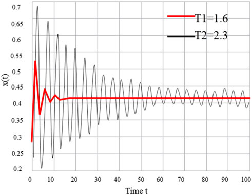
FiGURE 1. Numerical solution of Eq. 6 when 𝑉 = 3, 𝐶 = 7.

FIGURE 2

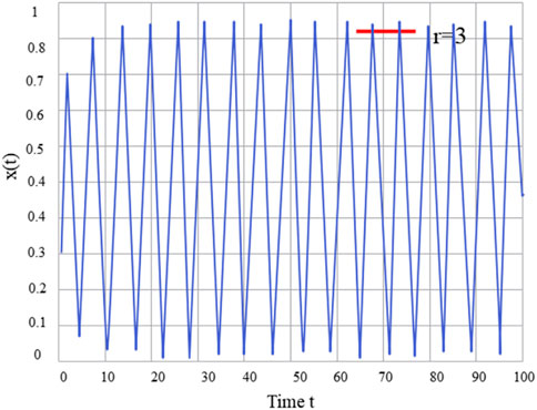
FIGURE 2. When 𝜏 = 3, the solution of Eq. 6 oscillates and does not converge.

Stability of evolutionary steady state under exponential kernel function

The stability of replication dynamics with bounded continuous time delays under constant kernel function is discussed. This section examines the stability of the evolutionary steady state when the kernel function has an exponential form. Note that the conclusions in this section are only a sufficient condition for the evolutionary stable state to be asymptotically stable. In fact, for general delay differential equations, it is difficult to obtain sufficient and necessary conditions for the stability of the solutions as in the previous section. This is the so-called conservative problem in the field of differential equations.

Below, we consider a replication dynamics model with bounded continuous distributed delays of the form.

$\frac{dx\left(t\right)}{dt}=-\alpha x\left(t\right)\left(1-x\left(t\right)\right)\left({\int }_{t-\tau }^t{e}^{-\left(t-s\right)}\left(x\left(s\right)-\overline{x}\right)ds\right)(12)$

Among them, $={\alpha }_1+{\alpha }_2,\overline{x}={\alpha }_2/\alpha ,{\alpha }_1=c-a,{\alpha }_2=b-d$ .

Note that in the above-mentioned time-delay evolution dynamics, the time-delay information at each moment is not equally important. The time lag information that is closer to the current time t has a greater impact on the current state. It can be said that the exponential kernel function is more general and more realistic than the constant kernel function. Similar to the discussion in the previous section, in order to examine the stability of the evolutionary stabilization strategy $\overline{x}$, this paper first substitutes the variable $y\left(t\right)=x\left(t\right)-\overline{x}$ to get:

$\frac{dy\left(t\right)}{dt}=-\alpha \left(y\left(t\right)+\overline{x}\right)\left(1-y\left(t\right)-\overline{x}\right){\int }_{t-\tau }^t{e}^{-\left(t-s\right)}y\left(s\right)ds(13)$

Then the stability study of the solution $x\left(t\right)\equiv \overline{x}$ of Eq. 12 is transformed into the stability study of the zero solution of Eq. 13.

Further, linearizing Eq. 13 around $\left(t\right)\equiv 0$ , we get:

$\begin{array}{l}\frac{dz\left(t\right)}{dt}=-\alpha \overline{x}\left(1-\overline{x}\right){\int }_{t-\tau }^t{e}^{-\left(t-s\right)}z\left(s\right)ds\\ =-\delta {\int }_{t-\tau }^t{e}^{-\left(t-s\right)}z\left(s\right)ds\end{array}(14)$

Among them, $\delta =\alpha \overline{x}\left(1-\overline{x}\right)$.

Similar to the discussion in the previous section, it is easy to obtain the feature equation of the linearized Eq. 14 as follows:

$\lambda +\delta {\int }_{-\tau }^0{e}^{\left(\lambda +1\right)s}ds=0,(15)$

That is,

${\lambda }^2+\lambda +\delta -\delta e^{-\tau \left(\lambda +1\right)}=0.(16)$

When the time delay $\tau$ is sufficiently small, the first-order Taylor expansion of the exponential term $e^{-\tau \left(\lambda +1\right)}$ in the feature Eq. 16 is carried out, and the above equation is converted into the following quadratic equation about.

${\lambda }^2+\left(1+\delta \tau \right)\lambda +\delta \tau =0(17)$

Theorem 2. For sufficiently small delays τ, the evolutionary stable state 𝑥¯ is asymptotically stable under replica dynamics (12) with bounded continuously distributed delays.

The two roots ${\lambda }_1$ and ${\lambda }_2$ of Eq. 17 satisfy:

$\begin{array}{l}{\lambda }_1+{\lambda }_2=-\left(1+\delta \tau \right)<0,\\ {\lambda }_1\cdot {\lambda }_2=\delta \tau >0\end{array}$

Therefore, the evolutionary stable state $\overline{x}$ is asymptotically stable under the replication dynamics (12) when the time lag is sufficiently small.

Next, for a general time-delay τ, we obtain a sufficient condition for the evolutionary stable state 𝑥¯ to be asymptotically stable under replication dynamics (12). We look forward to finding a larger upper bound for delay τ in future work, which involves the conservation of equations and is also one of the key issues in the study of delay differential equations.

Theorem 3. Under replication dynamics (12) with bounded continuously distributed delays, the evolutionary stable state $\overline{x}$ is asymptotically stable if $<\frac{\pi }{2\delta }$ .

Certification: $\lambda =u+iv$ is the root of the feature Eq. 15, where $,v\in \mathbb{R}$ . Then, according to the feature Eq. 15, we have

$\begin{array}{l}\lambda +\delta {\int }_{-\tau }^0{e}^{\left(\lambda +1\right)s}ds=u+iv+\delta {\int }_{-\tau }^0{e}^{\left(u+iv+1\right)s}ds\\ =u+iv+\delta {\int }_{-\tau }^0{e}^{\left(u+1\right)s}\cdot e^{\left(ivs\right)}ds\\ =u+iv+\delta {\int }_{-\tau }^0{e}^{\left(u+1\right)s}\left(\mathit{cos}vs+i\mathit{sin}vs\right)ds\\ =0\end{array}$

Separating the real and imaginary parts in the above formula, we get

$\begin{array}{l}u=-\delta {\int }_{-\tau }^0{e}^{\left(u+1\right)\sigma }\mathit{cos}v\sigma d\sigma \\ v=-\delta {\int }_{-\tau }^0{e}^{\left(u+1\right)\sigma }\mathit{sin}v\sigma d\sigma \end{array}$

If the real part of the characteristic root $\lambda =u+iv$ is assumed to be $\ge 0$ , then

$\begin{array}{l}\left|v\right|=\delta \left|{\int }_{-\tau }^0{e}^{\left(u+1\right)\sigma }\mathit{sin}v\sigma d\sigma \right|\\ \le \delta \left|{\int }_{-\tau }^0{e}^{\left(u+1\right)\sigma }d\sigma \right|\\ \le \delta \\ <\frac{\pi }{2\tau }\end{array}(18)$

Further, from the integral median theorem, we know that:

$\begin{array}{l}0\ge -\frac{1}{\delta }\cdot u={\int }_{-\tau }^0{e}^{\left(u+1\right)\sigma }\mathit{cos}v\sigma d\sigma \\ =\tau e^{\left(u+1\right){\sigma }^{*}}\mathit{cos}v{\sigma }^{*}\end{array}$

Among them, ${\sigma }^{*}\in \left[-\tau ,0\right]$ . Thereby

$2k\pi +\frac{\pi }{2}\le v{\sigma }^{*}\le 2k\pi +\frac{3\pi }{2},$

Among them, $\in \mathbb{Z}$ .

Note that by combining Eq. 18, we get:

$\left|v{\sigma }^{*}\right|\le \left|v\tau \right|<\frac{\pi }{2}.$

This is a contradiction. Therefore, the real part is u < 0. This shows that when $\tau <\frac{\pi }{2\delta }$ , the eigenvalues of the characteristic Eq. 15 all have negative real parts, so that the evolutionary stable state $\overline{x}$ is asymptotically stable under the replication dynamics (12) with bounded continuous distributed delays.

At the end of the previous section, we validated our results by numerical simulations of replication dynamics with a bounded continuous distributed delay under a constant kernel function against the background of the hawk-dove game model. Next, we give a simple example of replication dynamics (12) with bounded continuous time-delay under the exponential kernel function under the eagle-dove game model with the same parameters. We briefly restate the eagle-dove game model, and its game matrix is as follows.

$\begin{array}{ccc}& H& D\\ H& \frac{V-C}{2}& V\\ D& 0& \frac{V}{2}\end{array}$

Among them, C > 0, V > 0, V < C. Continuing from the previous section, when C = 7, V = 3, it is easy to calculate the evolutionary stable state $\overline{x}=0.428$ . It can be seen from Figure 3A that when the time delay $\tau$ is small, the solution of Eq. 12 converges to the evolutionary stable policy $\overline{x}$ . It is worth noting that the convergence rate is relatively slow at this time. It can be seen from Theorem two that the evolutionary stable state $\overline{x}$ is asymptotically stable when $<\frac{\pi }{2\delta }$ , and Figure 3B verifies our conclusion. However, since our conclusion is only a sufficient condition for asymptotic stability. Therefore, in the future work, how to theoretically enlarge the upper bound of the delay, that is, to reduce the conservatism of the integro-differential Eq. 12 will be a very meaningful work in terms of both the application of game theory and the theory of time-delay differential equations.

FIGURE 3

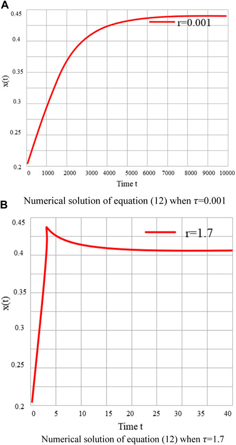
FIGURE 3. Simulation analysis diagram 3Prediction of groundwater pollution diffusion path based on multi-source data fusion. (A) Numerical solution of equation (12) when τ = .001; (B) Numerical solution of equation (12) when τ = 1.7).

In this paper, a method combining leaching surface and flux concentration is proposed, and a numerical simulation method is applied to simulate and analyze transient leakage monitoring of similar point and line source pollution in a planar two-dimensional heterogeneous aquifer. On the stratigraphic characteristic scale, the stochastic simulation method is used to generate the profile two-dimensional heterogeneous anisotropic aquifer. Under the conditions of convective dispersion and adsorption, the migration and evolution of polluted plumes in this special heterogeneous formation are analyzed by numerical simulation method, which provides a reference for the monitoring and management of such polluted aquifers. The prediction of groundwater pollution diffusion path based on the total multi-source data fusion in this paper is shown in Figure 4.

FIGURE 4

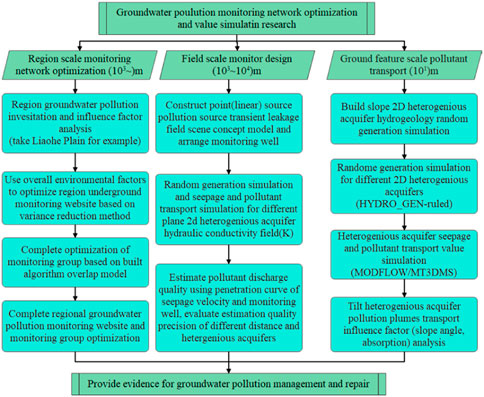
FIGURE 4. Groundwater pollution diffusion path based on multi-source data fusion.

Taking the identification of sudden pollution incidents as the ultimate goal, the four factors of environmental impact factors, emergency response factors, social impact factors, and groundwater system factors are used as the criterion layers. The identification index system of sudden pollution incidents is established by refining the supported indicators respectively, as shown in Figure 5. The selection of indicators in the indicator system is based on the principles of scientificity, systematicness, pertinence and operability.

FIGURE 5

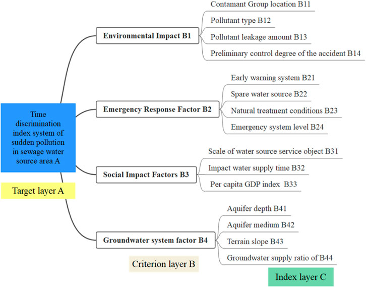
FIGURE 5. Indicator system for the identification of emergency disposal technologies for sudden pollution in groundwater sources.

In order to further verify the reliability of the established mathematical model and model parameters, the experimental analysis is carried out, and the study is carried out in a certain area, as shown in Figure 6. From the concentration fitting diagram in Figure 7, a total of 23 observation points is taken in the model identification stage. It can be seen that the isolines of the measured and calculated concentrations also achieve a good fit as a whole. It shows that the established hydrogeological conceptual model and mathematical model are reasonable.

FIGURE 6

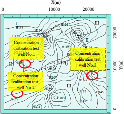
FIGURE 6. Example diagram of the study area.

FIGURE 7

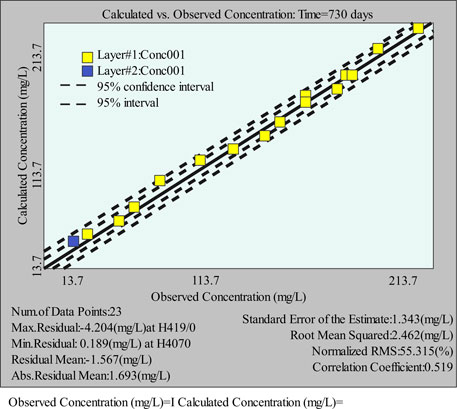
FIGURE 7. Concentration fitting diagram in the validation stage.

It is divided into six stress periods, and each 360 days is a stress period. From the inspection results, select three representative observation holes. It can be seen that the model identification and verification results prove that the established mathematical model, boundary conditions, hydrogeological parameters and source-sink terms are all reasonable, and the model can be used for the prediction of groundwater solute system (Figure 8).

FIGURE 8

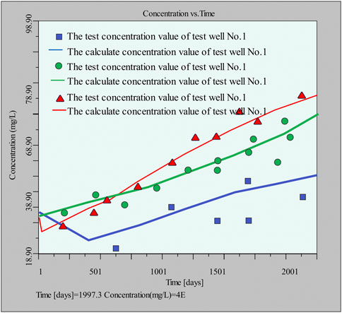
FIGURE 8. Fitting hydrograph of groundwater solute concentration in calibration monitoring well.

The above research verifies that the multivariate data fusion proposed in this paper can play an important role in the prediction of groundwater pollution diffusion paths.

Conclusion

In recent years, with the acceleration of industrialization and urbanization, the demand for water has increased dramatically. The unreasonable exploitation of groundwater resources has led to the continuous deterioration of regional water resources, the increasingly serious water pollution, and the increasingly prominent contradictions in urban water supply, industry, agriculture and animal husbandry. At present, environmental problems such as ground subsidence, ground fissures, and ground subsidence have occurred in many areas, which have seriously affected the lives of local people and greatly restricted local economic development. Groundwater pollution refers to the phenomenon that the quality of groundwater is degraded under the influence of human activities, thereby changing the physical properties, chemical composition and biological characteristics of water. This paper combines the multivariate data fusion technology to predict and analyze the groundwater pollution diffusion path to improve the prediction accuracy of the groundwater pollution diffusion path. The experimental study verifies that the multivariate data fusion proposed in this paper can play an important role in the prediction of the groundwater pollution diffusion path.

Data availability statement

The original contributions presented in the study are included in the article/supplementary material, further inquiries can be directed to the corresponding author.

Author contributions

YZ: supervision; investigation XH: investigation YL: writting.

Funding

National Natural Science Foundation of China (No. 42107093, 42062017, U1967209); Open Fund for State Key Laboratory of Nuclear Resources and Environment, East China University of Technology (No. NRE 1927); Open Fund for Fundamental Science on Radioactive Geology and Exploration Technology Laboratory, East China University of Technology (No. RGET 1904).

Conflict of interest

The authors declare that the research was conducted in the absence of any commercial or financial relationships that could be construed as a potential conflict of interest.

Publisher’s note

All claims expressed in this article are solely those of the authors and do not necessarily represent those of their affiliated organizations, or those of the publisher, the editors and the reviewers. Any product that may be evaluated in this article, or claim that may be made by its manufacturer, is not guaranteed or endorsed by the publisher.

References

Bakhoum, J. P., Diop, N. A., Bodian, E. H. T., Mbaye, O., Diaw, P., Cisse, L., et al. (2020). Development of an on-site early warning water quality monitoring system for pesticide detection by absorption and photo-induced fluorescence. Environ. Sci. Pollut. Res. 27 (36), 45238–45249. doi:10.1007/s11356-020-10406-x

PubMed Abstract | CrossRef Full Text | Google Scholar

Ballen, S. C., Ostrowski, G. M., Steffens, J., and Steffens, C. (2021). Graphene oxide/urease nanobiosensor applied for cadmium detection in river water. IEEE Sensors J. 21 (8), 9626–9633. doi:10.1109/jsen.2021.3056042

CrossRef Full Text | Google Scholar

Bayat, F., Didar, T. F., and Hosseinidoust, Z. (2021). Emerging investigator series: Bacteriophages as nano engineering tools for quality monitoring and pathogen detection in water and wastewater. Environ. Sci. Nano 8 (2), 367–389. doi:10.1039/d0en00962h

CrossRef Full Text | Google Scholar

Bezagio, R. C., Colli, C. M., Romera, L. I. L., de Almeida, C. R., Ferreira, É. C., Mattia, S., et al. (2020). Improvement in cyst recovery and molecular detection of Giardia duodenalis from stool samples. Mol. Biol. Rep. 47 (2), 1233–1239. doi:10.1007/s11033-019-05224-5

PubMed Abstract | CrossRef Full Text | Google Scholar

Chao, D., Chen, J., Dong, Q., Wu, W., Qi, D., and Dong, S. (2020). Ultrastable and ultrasensitive pH-switchable carbon dots with high quantum yield for water quality identification, glucose detection, and two starch-based solid-state fluorescence materials. Nano Res. 13 (11), 3012–3018. doi:10.1007/s12274-020-2965-8

CrossRef Full Text | Google Scholar

Cope, J. R., Kahler, A. M., Causey, J., Williams, J. G., Kihlken, J., Benjamin, C., et al. (2019). Response and remediation actions following the detection of Naegleria fowleri in two treated drinking water distribution systems, Louisiana, 2013–2014. J. water health 17 (5), 777–787. doi:10.2166/wh.2019.239

PubMed Abstract | CrossRef Full Text | Google Scholar

Domańska, M., Hamal, K., Jasionowski, B., and Łomotowski, J. (2019). Bacteriological contamination detection in water and wastewater samples using OD600. Pol. J. Environ. Stud. 28 (6), 4503–4509. doi:10.15244/pjoes/94838

CrossRef Full Text | Google Scholar

Fereidooni, Z., Tahayori, H., and Bahadori-Jahromi, A. (2021). A hybrid model-based method for leak detection in large scale water distribution networks. J. Ambient Intell. Humaniz. Comput. 12 (2), 1613–1629. doi:10.1007/s12652-020-02233-2

CrossRef Full Text | Google Scholar

Jongman, M., Carmichael, P. C., and Bill, M. (2020). Technological advances in phytopathogen detection and metagenome profiling techniques. Curr. Microbiol. 77 (4), 675–681. doi:10.1007/s00284-020-01881-z

PubMed Abstract | CrossRef Full Text | Google Scholar

Kaushik, M., Nandi, A. V., and Mungurwadi, V. B. (2018). Portable sensors for water pathogens detection. Mater. Today Proc. 5 (4), 10821–10826. doi:10.1016/j.matpr.2017.12.368

CrossRef Full Text | Google Scholar

Kitajima, M., Sassi, H. P., and Torrey, J. R. (2018). Pepper mild mottle virus as a water quality indicator. NPJ Clean. Water 1 (1), 19–9. doi:10.1038/s41545-018-0019-5

CrossRef Full Text | Google Scholar

Mabvouna Biguioh, R., Adogaye, S. B. B., Pete, N., Martial, P., Sanou Sobze, M., Kemogne, J. B., et al. (2020). Microbiological quality of water sources in the west region of Cameroon: Quantitative detection of total coliforms using micro biological survey method. BMC public health 20 (1), 346–347. doi:10.1186/s12889-020-8443-0

PubMed Abstract | CrossRef Full Text | Google Scholar

Motlagh, A. M., and Yang, Z. (2019). Detection and occurrence of indicator organisms and pathogens. Water Environ. Res. 91 (10), 1402–1408. doi:10.1002/wer.1238

PubMed Abstract | CrossRef Full Text | Google Scholar

Pandiarajan, S., Thambiratnam, S., and Sivaruban, I. R. B. (2019). Bio-monitoring and detection of water quality using Ephemeroptera, plecoptera and Trichoptera (EPT) complex in karanthamalai stream of eastern ghats. Indian J. Ecol. 46 (4), 818–822.

Google Scholar

Peng, J., Xia, C. Q., Xu, Y., Li, R., Cui, L., Clegg, J. K., et al. (2021). Crystallization of CsPbBr3 single crystals in water for X-ray detection. Nat. Commun. 12 (1), 1531–1610. doi:10.1038/s41467-021-21805-0

PubMed Abstract | CrossRef Full Text | Google Scholar

Rathi, S. (2021). S-PLACE ga for optimal water quality sensor locations in water distribution network for dual purpose: Regular monitoring and early contamination detection–a software tool for academia and practitioner. Water Supply 21 (2), 615–634. doi:10.2166/ws.2020.333

CrossRef Full Text | Google Scholar

Santonastaso, G. F., Di Nardo, A., Creaco, E., Musmarra, D., and Greco, R. (2021). Comparison of topological, empirical and optimization-based approaches for locating quality detection points in water distribution networks. Environ. Sci. Pollut. Res. 28 (26), 33844–33853. doi:10.1007/s11356-020-10519-3

PubMed Abstract | CrossRef Full Text | Google Scholar

Song, H., Zhou, Y., Li, Z., Zhou, H., Sun, F., Yuan, Z., et al. (2021). Inner filter effect between upconversion nanoparticles and Fe (ii)–1, 10-phenanthroline complex for the detection of Sn (ii) and ascorbic acid (AA). RSC Adv. 11 (28), 17212–17221. doi:10.1039/d1ra01925b

PubMed Abstract | CrossRef Full Text | Google Scholar

Tripathi, S. M., and Chaurasia, S. (2020). Detection of Chromium in surface and groundwater and its bio-absorption using bio-wastes and vermiculite. Eng. Sci. Technol. Int. J. 23 (5), 1153–1161. doi:10.1016/j.jestch.2019.12.002

CrossRef Full Text | Google Scholar

Tshamala, A. K., Musala, M. K., Kalenga, G. K., and wa Mumapanda, H. D. (2021). Assessment of surface water quality in kakanda: Detection of pollution from mining activities. J. Environ. Prot. 12 (9), 561–570. doi:10.4236/jep.2021.129035

CrossRef Full Text | Google Scholar

Zhang, Y., Yang, X., and Zhou, H. C. (2018). Direct synthesis of functionalized PCN-333 via linker design for Fe 3+ detection in aqueous media. Dalton Trans. 47 (34), 11806–11811. doi:10.1039/c8dt01508b

PubMed Abstract | CrossRef Full Text | Google Scholar