Longitudinal velocity profile of flows in open channel with double-layered rigid vegetation

Aquatic vegetation of different heights is widely scattered in natural rivers and is conducive to their environmental function while affecting the flow hydrodynamic conditions. A semi-analytical velocity model is constructed and used to study the longitudinal velocity profile in open channel flow through double-layered rigid vegetation. The double-layered vegetation flow is separated into three zones according to the velocity profile: 1) nearly uniform distributed velocity zone 1A in the lower region of the short vegetation layer, 2) a mixing layer zone B, 3) uniform distributed velocity zone 2A in the upper region of the tall vegetation layer. Two force equilibrium equations about the gravity-driving and vegetation drag are solved to obtain the uniform velocity distribution equations in zone 1A and 2A. The velocity of zone 1A and B is further modeled as a linear superposition of two concepts: the uniform velocity distribution term of zone 1A and a hyperbolic tangent profile. Meanwhile, longitudinal velocity and the lateral vorticity profiles of open channel flow through double-layered rigid vegetation are studied by laboratory flume tests of different vegetation arrangements exposed to two water depths and three slopes. The experimental results show that the longitudinal velocity increases with the slope increase. The verification of the velocity model is based on the instantaneous velocity measured by Acoustic Doppler Velocimetry (ADV), which shows acceptable agreement, indicating that the model can give a reference to the longitudinal velocity of multi-layered vegetation flow in some cases. The effects of wake vortices and boundary friction on the model are further explored in the discussions. The results presented in this study could contribute to the management of aquatic vegetation configurations and the restoration of freshwater ecology.

1 Introduction

Aquatic vegetation is widely distributed in the riffles and shallow water areas of rivers, forming a more complex hydrodynamic system than the bare channel. Vegetation increases the flow resistance, raises the water level, reduces the flow capacity, alters the local flow dynamic characteristics and sediment sorting process, and thus influences the erosion and geomorphic evolution of the river (Yang et al., 2015; Huai et al., 2019; Li et al., 2020). Meanwhile, vegetation is also beneficial to the freshwater ecosystem. For example, aquatic plants can enhance the water quality by absorbing or degrading some harmful substances and can shelter the aquatic microorganisms and fish in the river (Xu and Nepf, 2020; 2021; Huai et al., 2021). Sometimes, vegetation increases the transparency of the water by reducing the flow velocity and enhancing the deposition of suspended sediment (Liu and Nepf, 2016). Vegetation roots can consolidate the riverbed soil and improve the bank stability to prevent excessive flow erosion (Qu, 2014). Since the appropriate arrangement of vegetation impacts the ecological process on land-freshwater ecosystems, the bioremediation technology of planting vegetation in river channels has been widely applied (Zhang, 2014). Analyzing the hydrodynamic characteristics and establishing accurate flow velocity models provide a scientific basis for water environment management and restoration of rivers and streams (Wang et al., 2021). Therefore, it is of great practical significance to study the hydrodynamic structure within the vegetation, which helps predict the flood hazards and restore the freshwater ecosystem.

Vegetated flow is generally divided into single-layered or double-layered vegetation flow, where the aquatic vegetation is emergent or submerged (Huai et al., 2021). Numerous studies have revealed the hydrodynamic characteristics of open channel flow with single-layered vegetation by investigating the vegetation flexibility, density, leaf area, and stem diameter (Velasco et al., 2003; Cheng, 2013; Zhang et al., 2020). The study on vegetation drag coefficient also extends from individual plants to vegetation arrays and from rigid vegetation to flexible vegetation (Tang et al., 2007; Chen et al., 2013). Redefining some parameters in vegetated flow compared to the bare bed is utility to quantify the flow characteristics. For example, a new model of the friction factor f in the vegetated flow concerned about the vegetation turbulence is more reasonable compared with the Darcy-Weisbach formula (Wang et al., 2019a), where the friction factor f is vital in the bulk velocity prediction of the flow with rigid or flexible vegetation (Wang et al., 2020).

In rivers, flexible vegetation accounts for much aquatic vegetation, so the flow through flexible vegetation has been widely concerned in recent years. Flexible vegetation will bend and deform under the influence of water flow, meanwhile, the deformation of vegetation affects the flow characteristics, resulting in a complex turbulence structure and redistribution of flow velocity (Kubrak et al., 2008; Zhang and Lai, 2015; Zhang et al., 2020). The flow structure is more complicated when consider the geometry of the plant shape (Wang et al., 2019b), and it is usually using rigid cylinders to represent the aquatic plants with fewer leaves in numerous studies (Huai et al., 2021), the study here also simulates the vegetation with rigid material.

In the flow through single-layered submerged vegetation, the vertical profile of longitudinal velocity no longer follows the law of logarithmic distribution from the bed to the free water surface, but can be divided into two layers, i.e., the vegetation layer and the free-water layer, or divided into three layers by adding a mixing layer between the vegetation layer and the free-water layer (Zhang, 2014). The longitudinal velocity through the flexible vegetation conforms to the “C” distribution while conforming to the “J” distribution above the vegetation layer (Fan et al., 2020). For the emergent canopy, the vegetation-bed-flow coherent structures affect the near-bed flow region, which is so called the effective bottom boundary, causing the flow velocity to increase from the bed, reach a peak, and decline to a constant value above this layer (Tseng et al., 2021). In addition to flow through the vegetation of uniform arrangements, the flow characteristic in a channel partially covered with vegetation array or fully covered with compound vegetation patterns has been studied. Zhang et al. (2021) derived the theoretical solutions of longitudinal velocity from the momentum model of a two-zone vortex structure in a channel partially covered with vegetation. Li et al. (2022) explored the characteristics of open channel flows with two layout patterns of rigid-flexible and flexible-rigid vegetation.

However, the vegetation in natural rivers often shows different heights. Both submerged and emergent vegetation are widely distributed in floodplains or shallow water (Zhao et al., 2015). Numerous experimental, numerical, and analytical researches on the hydrodynamic structure of double-layered vegetation flow were conducted. When both vegetation layers are submerged, according to the longitudinal velocity profile, the double-layered vegetation flow is separated into a short vegetation layer, a tall vegetation layer, and a free-water zone (Huai et al., 2014). Each vegetation layer is divided into an upper vegetation zone and a lower vegetation zone, in which the velocity of lower vegetation zones is constant and increases in upper vegetation zones and free-water zone (Liu et al., 2010; Huai et al., 2014; Zhao, 2017; Wang Z. et al., 2019; Rahimi et al., 2020; Tang et al., 2021). Under different vegetation arrangements, densities, vegetation height, and flow depths, the velocity, turbulence intensity, the flow resistance, and the vorticity of double-layered vegetation flows were found more complex than single-layered vegetation flow (Liu et al., 2010; Wang Z. et al., 2019; Rahimi et al., 2020). Therefore, considering the effect of the double-layered vegetation, an analytical model of the longitudinal velocity was proposed basing on the momentum balance equation (Huai et al., 2014), and the hydraulic radius formula and Manning coefficient formula were modified (Tang et al., 2021).

Above all, it is more common that the aquatic vegetation has two or more different heights in natural rivers. Most studies of double-layered rigid vegetation flow focused on the vertical or longitudinal distribution of flow velocity, Reynolds stress, and turbulence intensity. Only a few studies are concerned about using a formula to describe the flow velocity profile under different vegetation arrangements and slopes, and this is also initial to understand the characteristics of flow with multiple-layered vegetation. This paper aims to study the flow characteristics of the double-layered rigid vegetation flow with different water depths, slopes, and vegetation densities. By subdividing the flow into distinct zones, listing the force balance equations, and using the superposition method to describe the momentum transport of the mixing layer, a longitudinal velocity model of the open-channel flows with double-layered rigid vegetation is proposed and verified by the experimental data. The laboratory flume tests use Acoustic Doppler Velocimetry (ADV) to collect three-dimensional velocity. The results can provide guidance for vegetation arrangements in channels, the construction of ecological rivers, and support river environment management and restoration.

2 Theoretical analysis

The steady and uniform open-channel flow with double-layered rigid vegetation composed of short and tall cylindrical stems with the height of h₁ and h₂ is generally separated into two cases in previous studies according to the water depth H, i.e., H > h₂ or h₁ < H < h₂. In this paper, we only study the case of h₁ < H < h₂. Using layer 1 and layer 2 to respectively denote the short and tall vegetation layer, Huai et al. (2014) suggested that in the case of h₁ < H< h₂, the flow can be separated into three zones according to the longitudinal velocity profile, i.e., lower zone of layer 1 marked as zone 1A (z < h₁-h_u), mixing layer zone marked as zone B at the upper region of layer 1 (h₁-h_u < z < h₁), and tall vegetation layer marked as zone 2A (h₁ < z < H), where h_u is the height of zone B and the upper edge of zone B coincides the top of layer 1. While the mean velocities in zone 1A and zone 2A are nearly constant, it significantly increases in zone B.

According to the study of mixing layer in the submerged vegetation (Nikora et al., 2013), the mean velocity can be obtained by a (quasi-)linear superposition of individual mechanisms acting in the double-layered vegetated flow at zone 1A and zone B, taking two concepts into account, i.e., (1) a uniform velocity distribution within zone 1A with a constant value (U_UD1), and (2) a mixing layer concept generated by the Kelvin-Helmholtz instability (U_ML). Besides, the velocity of zone 2A is expressed as a constant velocity profile (U_UD2) in brief. The conceptual velocity model for flows with double-layered rigid vegetation is outlined in Figure 1. Assuming the upper inflection point (marked z₂) of zone B is slightly above the canopy of the short vegetation layer, and our experimental results will verify this assumption. The lower inflection point of the mixing layer zone in the short vegetation layer is marked as z₁, ${\delta }_{\mathrm{w}}=z_2-z_1$ is the height of the mixing layer.

FIGURE 1

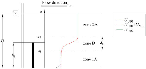
FIGURE 1. Conceptual model for flows with double-layered rigid vegetation.

For a unit canopy volume in vegetated flow, the vegetation drag can be calculated as (Huai et al., 2014):

$\begin{array}{c}{F}_{\mathrm{d}}=\frac{1}{2}\rho C_{\mathrm{D}}mD{u}^2,\end{array}(1)$

where $\rho$ (kg·m⁻³) is the water density, C_D is the vegetation drag coefficient, m is the number of stems per bed area, D (m) is the diameter of the vegetation stem, and u (m·s⁻¹) is the mean velocity of the flow.

The force equation of a small length-scale dx along the streamwise direction in zone 1A can be expressed as a balance of the gravity-driving term, vegetation drag term, bed friction term, and the sidewall friction term:

$\begin{array}{c}\rho gi\left(1-{\lambda }_1\right)W{z}_{1}dx=\frac{1}{2}\rho C_{\mathrm{D}}{m}_{1}D{U_{\mathrm{U}\mathrm{D}1}}^{2}W{z}_{1}dx+{\tau }_{\mathrm{b}\mathrm{e}\mathrm{d}}\left(1-{\lambda }_1\right)Wdx+2z_1{\tau }_{\mathrm{w}\mathrm{a}\mathrm{l}\mathrm{l}}dx.\end{array}(2)$

Meanwhile, the force balance equation in zone 2A can be expressed as:

$\begin{array}{c}\rho gi\left(1-{\lambda }_2\right)W\left(H-z_2\right)dx=\frac{1}{2}\rho C_{\mathrm{D}}{m}_{2}D{U_{\mathrm{U}\mathrm{D}2}}^{2}W\left(H-z_2\right)dx+2\left(H-z_2\right){\tau }_{\mathrm{w}\mathrm{a}\mathrm{l}\mathrm{l}}dx.\end{array}(3)$

where the gravity-driving term on the left side of the Eqs 2, 3 considers the existence of the vegetation, g (m·s⁻²) is the gravity acceleration, i is the energy slope equaling to the bed slope J in open-channel flow, W (m) is the flume width, m₁ (plant·m⁻²) is the density of the short vegetation layer (including the short stems and the tall stems embedded in layer 1), m₂ (plant·m⁻²) is the density of the tall vegetation layer (only the tall stems in layer 2), U_UD1 (m·s⁻¹) is the uniform velocity in zone 1A, U_UD2 (m·s⁻¹) is the uniform velocity in zone 2A, ${\lambda }_1=\frac{m_1{D}^2\pi }{4}$; ${\lambda }_2=\frac{m_2{D}^2\pi }{4}$ are the solid volume fractions of the cylinders in the short and tall vegetation layers, respectively. Darcy-Weisbach formula ${\tau }_{\mathrm{b}\mathrm{e}\mathrm{d}}=\frac{1}{8}\rho U^2{f}_{\mathrm{b}\mathrm{e}\mathrm{d}}$ (kg·m⁻¹·s⁻²) and ${\tau }_{\mathrm{w}\mathrm{a}\mathrm{l}\mathrm{l}}=\frac{1}{8}\rho U^2{f}_{\mathrm{w}\mathrm{a}\mathrm{l}\mathrm{l}}$ (kg·m⁻¹·s⁻²) represents the shear stress produced by the bed and sidewalls, using the roughness parameter $f_{\mathrm{b}\mathrm{e}\mathrm{d}}$: and $f_{\mathrm{w}\mathrm{a}\mathrm{l}\mathrm{l}}$ to calculate, respectively (Wang et al., 2015).

Among the several terms in Eqs 2, 3, the bed friction $\left[{\tau }_{bed}\left(1-{\lambda }_1\right)Wdx\right]$ and the sidewall friction $\left[2z_1{\tau }_{wall}dx\right]$, $\left[2\left(H-z_2\right){\tau }_{wall}dx\right]$ are negligible since they are significantly lower than the vegetation drag, and the impact of the boundary stress terms is later discussed in Section 6.2. Then Eqs 2, 3 can be simplified as momentum equations:

$\begin{array}{c}\rho gi\left(1-{\lambda }_1\right)-\frac{1}{2}\rho C_D{m}_{1}D{U_{\mathrm{U}\mathrm{D}1}}^2=0,\end{array}(4)$

$\begin{array}{c}\rho gi\left(1-{\lambda }_2\right)-\frac{1}{2}\rho C_D{m}_{2}D{U_{\mathrm{U}\mathrm{D}2}}^2=0.\end{array}(5)$

The uniform distributed velocity term within the layer 1 can be expressed as:

$\begin{array}{c}{U_{\mathrm{U}\mathrm{D}1}=\left(\frac{gi\left(1-{\lambda }_1\right)}{0.5{DC}_D{m}_1}\right)}^{1/2},\end{array}(6)$

The velocity profiles in zone 2A can be expressed as:

$\begin{array}{c}{U}_{2\mathrm{A}}={U_{\mathrm{U}\mathrm{D}2}=\left(\frac{gi\left(1-{\lambda }_2\right)}{0.5{DC}_D{m}_2}\right)}^{1/2}.\end{array}(7)$

The vegetation density significantly differs between the short and tall vegetation layers. The vegetation drag in zone 1A is more significant than that in zone 2A due to its large density, leading to a prominent velocity gradient in zone B, which derives the generation of Kelvin-Helmholtz vortices there (Liu et al., 2010). Therefore, the Reynolds stress should be considered in the momentum equation. Assuming the mixing layer velocity term U_ML is a hyperbolic tangent profile:

$U_{\mathrm{M}\mathrm{L}}=\left(U_{z_2}-U_{\mathrm{U}\mathrm{D}1}\right)\bullet \left[1+\tan h\left(\frac{z-z_2}{{\delta }_{\mathrm{w}}}\right)\right].(8)$

where $U_{z_2}$ is the velocity at the inflection point z₂, equaling to $U_{\mathrm{U}\mathrm{D}2}$. And then, the velocity in zone 1A and zone B can be expressed as the superposition of the uniform distribution of the zone 1A and the hyperbolic tangent profile term:

$\begin{array}{c}{U}_{1\mathrm{A},B}=U_{\mathrm{U}\mathrm{D}1}+U_{\mathrm{M}\mathrm{L}}={\left(\frac{gi\left(1-{\lambda }_1\right)}{0.5{DC}_{\mathrm{D}}{m}_1}\right)}^{1/2}+\left[{\left(\frac{gi\left(1-{\lambda }_2\right)}{0.5{DC}_{\mathrm{D}}{m}_2}\right)}^{1/2}-{\left(\frac{gi\left(1-{\lambda }_1\right)}{0.5{DC}_{\mathrm{D}}{m}_1}\right)}^{1/2}\right]\bullet \left[1+\tan h\left(\frac{z-z_2}{{\delta }_{\mathrm{w}}}\right)\right].\end{array}(9)$

3 Experiments

3.1 Experimental settings

The experiments were conducted in a recirculating, free-surface flow flume at the Hydraulics Laboratory of the School of Soil and Water Conservation at Beijing Forestry University. The flume was 12.4 m long (L), .3 m wide (W), and .25 m deep (H₀). The electromagnetic flowmeter system controlled the discharge. At the same time, a honeycomb-shaped straightener at the inlet and an adjustable weir gate at the end of the flume were used to set a stable and uniform flow.

The vegetation was simulated with plastic cylinders of .006 m diameter (D), and the cylinders representing short vegetation and tall vegetation were .07 m (h₁) and .18 m (h₂), respectively. The cylinders were embedded in five 1 m long, .3 m wide, and .5 cm thick plexiglass plates. The vegetation section was 5-m-long, and the leading edge was 2.5 m from the flume inlet (see Figure 2A). A Cartesian coordinate is established with the frontal edge of the vegetation section as the origin. The x, y, and z coordinates denote streamwise, lateral, and vertical directions, respectively. The preliminary experiment of double-layered vegetation flow was conducted, the velocities at x = 0, .5, 1.3, 2.5, 3.6, and 4.5 m were measured, and the results showed that the longitudinal velocity at x = 3.6 m and x = 4.5 m had high consistency which means the flow behind x = 3.6 m is fully developed. Therefore, the velocity was measured at x = 4.0 m, representing the velocity of the fully developed region. Several cylinders were removed in order to measure the velocity using ADV. A side-view image of the double-layer model plants and velocity measurements for run XHS1 are shown in Figure 2B.

FIGURE 2

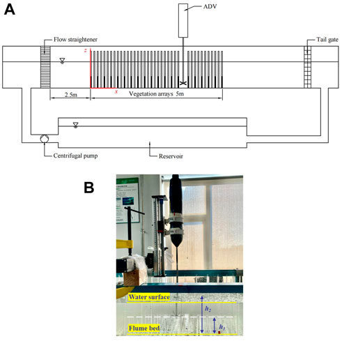
FIGURE 2. Experimental arrangement: (A) Sketch of the laboratory recirculating flume setup, the black part of the vegetation section represents the short cylinder; (B) A photo of the experiment for run XHS1, where short cylinders (h₁) are submerged and tall cylinders (h₂) are emergent.

3.2 Experimental conditions

The specific parameters of each run are given in Table 1. The experiments include two vegetation arrangements marked as X and Y, with different density ratios α = m₁/m₂. The water depth was set as a higher submergence state H = 14.00 cm (HS), and a lower submergence state H = 12.80 cm (LS), under which condition the short vegetation layer was submerged and the tall vegetation layer was emergent. The numbers 1-3 denoted three different slopes J, .001, .002, and .003. According to the Reynolds number Re=(U_mR)/ν and the Froude number F_r=U_m/$\sqrt{gH}$ , the experimental flow is turbulent and subcritical flow, where U_m = Q/WH is the average velocity over the section, R=(H-λ₁h₁-λ₂H)/(m₁h₁D + m₂HD) is the hydraulic radius of the half-submerged double-layered vegetation flow without consideration of the impact of the bed and walls (Tang et al., 2021), H is the water depth, Q is the flow discharge, g = 9.81 ms⁻² is the acceleration of the gravity, ν = 1.01 × 10⁻⁶ m²s⁻¹ is the kinematic viscosity of the water (based on the kinematic viscosity of the water under 101.325 kPa and 20°C).

TABLE 1

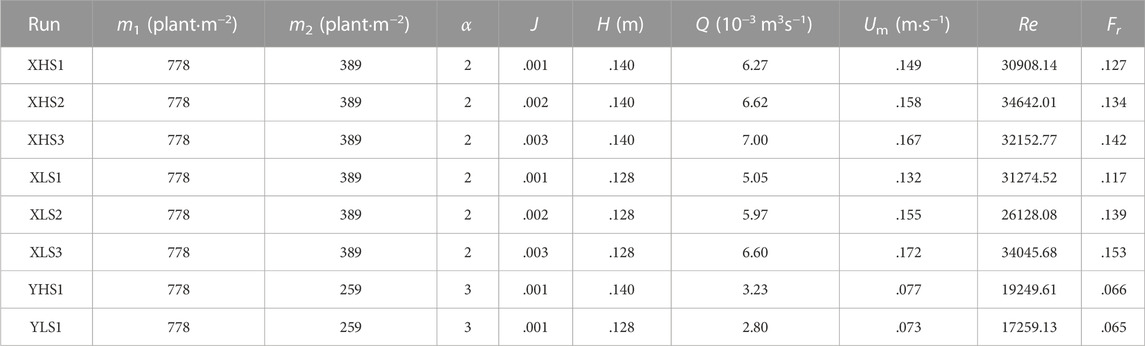
TABLE 1. Experimental parameters of each run.

3.3 Data collection and processing

Nortek Acoustic Doppler Velocimetry (ADV) was used to measure the instantaneous velocities. The ADV has one transmitting probe and four receiving probes. The transmitting probe in the center emits acoustic signals, and then receiving probes receive the acoustic frequency changes caused by the reflection or scattering of moving particles in the water to collect the data of the sampling body 5 cm in front of the probe. After the signal is processed by the system, the instantaneous velocity, signal intensity, signal-to-noise ratio (SNR), and correlation (COR) of each measuring point can be converted into a text file for output. The ADV cannot accurately measure the range of 2–3 cm below the water surface, for the upper signal-receiving probe will be emergent. The data acquisition frequency was 200 Hz, the sample volume was 5.5 mm³, and the sampling time was 40 s. Before the experiment, the ADV was fixed on a support. The tracer particles used in the experiment are hollow plexiglass beads of 20 µm diameter, and the density is .9 gcm⁻³. Figure 3 shows that there were three measuring locations in runs X representing behind the tall cylinder (BT), free stream behind the tall and short cylinders’ gap (BTS) and the short cylinder (BS), and one more for runs Y: Free stream behind two short cylinders’ gap (BSS). The measurement was done from the bed (z = .005 m) towards the free water surface with an increment of .005 m at each measuring location.

FIGURE 3

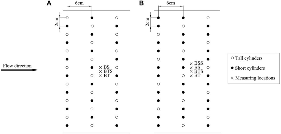
FIGURE 3. The arrangement of vegetation and measuring locations of (A) runs X and (B) runs Y. Black and white circles representing short and tall cylinders respectively, and the crosses represent measurement locations.

Python processed the experimental data. The longitudinal, lateral, and vertical instantaneous velocities with a signal-to-noise ratio (SNR) greater than 15 and correlation (COR) greater than 70% are regarded as valid data, and the time-average velocity of x, y, and z direction $\overline{u}$, $\overline{v}$, and $\overline{w}$ are obtained by time averaging the instantaneous velocities. The time-average longitudinal velocity of each measuring location was averaged horizontally to obtain the mean longitudinal velocity of the measuring cross-section.

4 Results

4.1 Longitudinal velocity profiles at different measurement locations

Figure 4 shows the longitudinal velocities at different locations of runs X and Y, and the black dotted line indicates the height of short vegetation h₁ = .07 m. The longitudinal velocity profile can be roughly divided into three zones, as mentioned above. Zone 1A is from the bed to z = .055 m (0 < z ≤ .79h₁), which is called the constant velocity zone, the velocity almost stays constant or has an insignificant increasing tendency. Zone B is from z = .055 m to z = .07–.08 m (.79h₁< z ≤ 1.14h₁). The velocity reaches the maximum at the top of the short vegetation or a slightly higher place and basically remains constant at zone 2A (1.14h₁< z ≤ 1.71h₁). The zoning of the longitudinal velocity profile is almost the same as the previous experimental results (Liu et al., 2010; Huai et al., 2014; Tang et al., 2021).

FIGURE 4

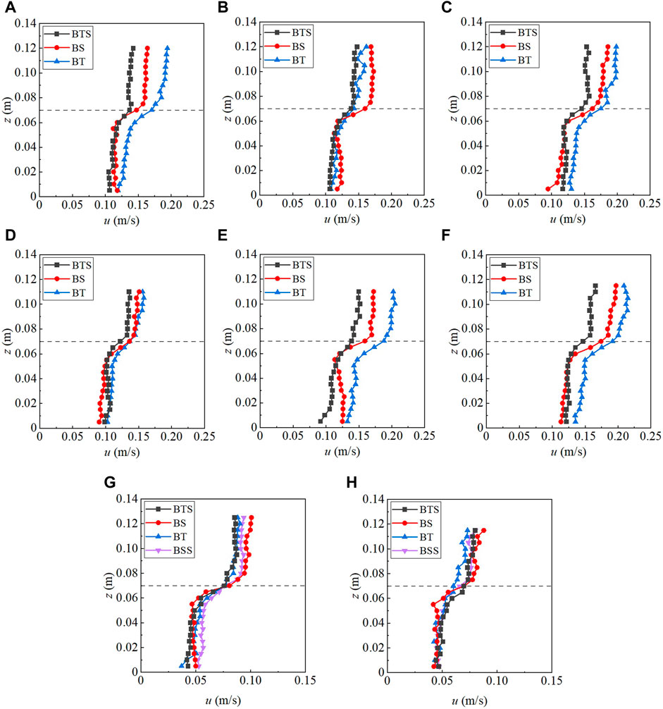
FIGURE 4. Vertical profiles of longitudinal velocity at different measurement locations for runs X and runs Y, (A–C) present results for runs XHS1 to XHS3, (D–F) present results for runs XLS1 to XLS3, (G,H) present results for runs YHS1 and YLS1, respectively. The black dotted line represents the height of the short cylinders.

Figure 4 shows that, except for run XHS2, the longitudinal velocity at location BT in runs X is the largest, and the one at location BTS is the smallest. The velocity at location BT in run XHS2 ranges between the value of location BS and location BTS, which is different from the regularities of the other runs, probably due to the error caused by an experimental operation, such as the slight deviation of the measurement location. Furthermore, in runs XHS1, XLS2, and XLS3, the velocities at locations BT and BTS have a percentage variance of 5%–18%. This is most likely due to the fact that the increasing of velocity component caused by the wake vortices after stem, based on the velocity model of linear superposition (Nikora et al., 2013). In runs Y, the velocity profiles at different locations are similar, and the velocity curve is not as smooth as that of runs X, especially the measured data of run YLS1, possibly due to the more complex arrangement of the vegetation cylinders of runs Y, leading to the frequent fluctuation of the velocity.

4.2 Mean longitudinal velocity of each run

Figure 5 displays the dimensionless mean longitudinal velocity of the measuring cross-section in each run. Every dimensionless velocity shows consistent distribution characteristic of “constant-increasing-constant” in vertical. For runs X, the velocity in zone 1A (u_1A) have a magnitude of .69–.83U_m and the velocity in zone 2A u_2A = .97–1.17U_m. For runs Y, the velocity in zone 1A u_1A = .59–.76U_m, and the velocity in zone 2A u_2A = 1.04–1.35U_m. The density ratio α of the double-layer vegetation under the same water depth and slope condition dictates the magnitude of the constant velocity within it. Here, the discharge Q is also an important factor affecting the velocity within the upper layer.

FIGURE 5

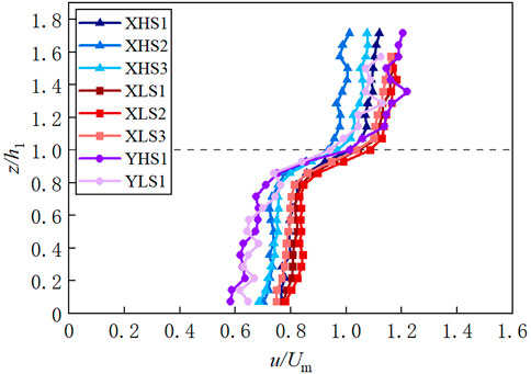
FIGURE 5. Vertical profile of the dimensionless mean longitudinal velocity for each run. The black dotted line represents the height of the short cylinders.

We define that the ratio of the mean velocity in zone 2A to the mean velocity in zone 1A $\beta =\overline{u_{2A}}/\overline{u_{1A}}$, where $\overline{u_{2A}}$ and $\overline{u_{1A}}$ is the mean experimental velocity of zone 2A and zone 1A, respectively. The α of runs Y is greater than runs X, leading to a more significant difference between the vegetation resistance and velocity distribution in zones 1A and 2A, and β of runs Y is 1.59–1.80. Table 1 shows that the velocity increases with the channel slope under the condition of the same vegetation arrangement and water depth. It can also be concluded from Figure 5 that the slope does not have much effect on the velocity ratio between zones 2A and 1A, the β of runs XHS and XLS are similar as the slope changes.

4.3 Lateral vorticity

The inflection point of the velocity profile in vegetated flows can be characterized by the lateral vorticity, and it can be calculated as the following equation (Singh et al., 2019):

$\omega =\frac{\partial w}{\partial x}-\frac{\partial u}{\partial z},(10)$

where the fluctuation of the vertical velocity $\partial w/\partial x$ is much weaker than the streamwise fluctuation $\partial u/\partial z$, so the term $\partial w/\partial x$ is neglected in the present calculation. The lateral vorticity profile is shown in Figure 6. In Figures6A–G, the lateral vorticity basically stays constant, being about zero in the lower zone of the short vegetation layer and upper zone of the tall vegetation layer, and there is a spike at the junction of short and tall vegetation layer. It shows that the momentum exchange in zone B is distinctly larger than in zones 1A and 2A. The results are similar to the lateral vorticity profiles of single-layered rigid vegetation flow found in Liu et al. (2008), and double-layered vegetation flow of Liu et al. (2010) and Singh et al. (2019). The vorticity distribution perfectly corresponds to the velocity distribution in Figure 4. The lateral vorticity profiles of run YLS1 show a strong fluctuation in zones 1A and 2A, and there is an exceptional value in run XHS2 at z = .115 m, possibly due to the experimental error at some measurement points.

FIGURE 6

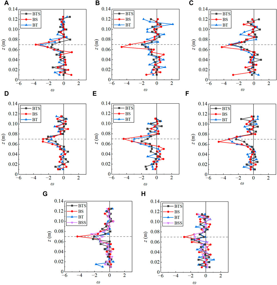
FIGURE 6. Lateral vorticity profile of different measurement locations, (A–C) present results for runs XHS1 to XHS3, (D–F) present results for runs XLS1 to XLS3, (G,H) present results for runs YHS1 and YLS1, respectively. The black dotted line represents the height of the short cylinders.

5 Application of the velocity model

5.1 Velocity model validation and error analysis

The application of the velocity model should base on the determination of the two parameters: The length scale of the mixing layer zone B (${\delta }_{\mathrm{w}}$) and the vegetation drag coefficient (C_D).

For simplicity, the deflection points of the mixing layer are determined using the method in Truong et al. (2019), which is used to define the edge of the penetration length in the vegetated zone and non-vegetated zone. The deflection points z₁ and z₂ are defined as the streamwise velocity $u_{z_1}=\left(1+5\%\right)\bullet \overline{u_{1\mathrm{A}}}$ and $u_{z_2}=\left(1-5\%\right)\bullet \overline{u_{2\mathrm{A}}}$, respectively.

The drag coefficient is calculated using the measurement data in zone 1A:

$\begin{array}{c}{C}_{\mathrm{D}}=\frac{gi\left(1-{\lambda }_1\right)}{\frac{1}{2}D{m}_1{\overline{u_{1\mathrm{A}}}}^2}.\end{array}(11)$

In runs X, the velocity model almost agrees well with the experimental data (Figures 7A–F), but underestimates or overestimates the velocity of zone 2A in runs Y (Figures 7G, H).

FIGURE 7

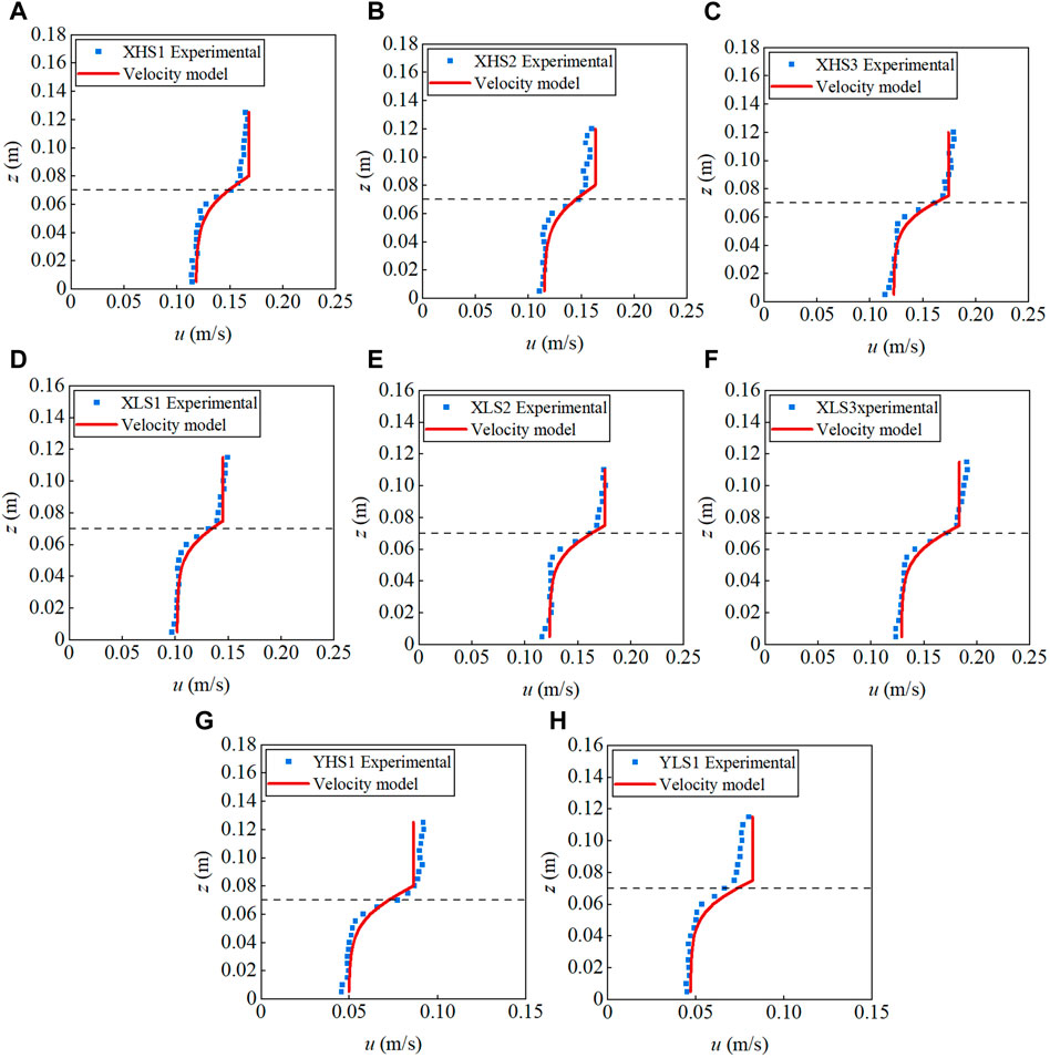
FIGURE 7. The velocity profile of the experimental data and predicted model for runs X and runs Y, the black dotted line represents the height of the short cylinders. (A-F) present results for runs X, and (G, H) present results for runs Y.

Moreover, in order to intuitively present the deviation of the predicted velocity from the measured velocity, the relative error (RE) is defined as follow:

$\begin{array}{c}RE=\frac{\left|U_{\mathrm{mod}}-u_{\mathrm{m}\mathrm{e}\mathrm{a}}\right|}{u_{\mathrm{m}\mathrm{e}\mathrm{a}}}.\end{array}(12)$

where U_mod is the predicted velocity of the model, and u_mea is the measured velocity. Figure 8 shows the RE at each measuring point of runs X along the water depth. The RE are relatively small in general, indicating that the model is a good reflection of the flow velocity profile. However, the RE in the near-bed 1 cm zone, zone B and zone 2A are larger than those in zone 1A, because the constant velocity model in zone 1A cannot catch the influence of boundary conditions precisely, and the entire velocity model is dependence on the C_D and ${\delta }_{\mathrm{w}}$ determined by the measurement data in zone 1A, leading to a higher RE in zone B and 2A.

FIGURE 8

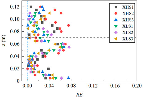
FIGURE 8. Relative error between the analytical model and the experimental velocity of runs X. The black dotted line represents the height of the short cylinders.

It is mentioned in Section 4.2 that the slope does not contribute to β, and the velocity model of zone 2A applied here denotes that the uniform velocity term difference between zone 2A and zone 1A is only related to the density of two vegetation layers, i.e., $U_{\mathrm{U}\mathrm{D}2}/U_{\mathrm{U}\mathrm{D}1}=\sqrt{\alpha \left(1-{\lambda }_1/1-{\lambda }_2\right)}$, the calculated values of runs X and runs Y are 1.406 and 1.715 respectively, while the β of runs X is 1.35–1.44, and 1.59–1.80 of runs Y. Therefore, it shows a small deviation in the modeling of the velocity in zone 2A. The model application results also verify that the longitudinal velocity in double-layered rigid vegetation flow follows a hyperbolic tangent distribution in the mixing layer as the distribution in single-layered submerged flexible vegetation flow, which may extend to the prediction of the mixing layer velocity in multi-layered vegetation flow; for instance, the velocity in a mixing layer can be expressed as the linear superposition of a uniform velocity in the lower layer and a hyperbolic tangent profile.

5.2 Relationship between C_D and the U_UD1 term

The C_D of this paper was estimated from the flow condition in zone 1A, and the dependence of the C_D on the stem Reynolds number of zone 1A Re_UD1=(U_UD1D)/ν for runs X is illustrated in Figure 9. It shows that C_D decreases as the Re_UD1 increases and has an increasing tendency to a growing slope J. This trend is probably due to the vortices penetrating deeper into the vegetation, and the gravitational component of the water along the slope direction is more significant with an increased slope, creating a more considerable vegetation drag. The results are consistent with the experimental data of single-layered submerged vegetation flow published in Nikora et al. (2013).

FIGURE 9

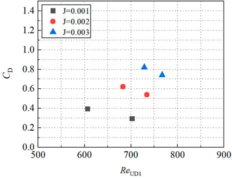
FIGURE 9. Dependence of the C_D on the Reynolds number of zone 1A for runs X.

6 Discussion

6.1 Edge of the mixing layer

This study is concerned with the influence of vegetation on the gravity-driving term compared with the velocity model proposed by Huai et al. (2014). The upper inflection point z₂ of the mixing layer is found above the top of the short vegetation canopy, while this point appears at the height of short vegetation in study of Huai et al. (2014). It is learned that the penetration length scale will change in different situations. The dense vegetation density (m₁ = 778 plant·m⁻²) in this study may cause larger scale coherent vortices and thus penetrate to the tall vegetation layer, compared with the sparse vegetation density (m₁ = 117 plant·m⁻²) in Huai et al. (2014); Figure 6 shows that the lateral vorticity reaches a peak at the height of short vegetation and decreases to zero near z = .075–.08 m, verifying the existence of the large-scale Kelvin-Helmholtz vortices. Moreover, according to Figures 4E, 8A in the study of Anjum and Tanaka (2020), the Reynolds stress turbulence model of double-layered vegetation flow indicates that the mixing region affected by the vertical coherent vortices contains the zone in short vegetation layer and tall vegetation layer, it is reasonable to assume that the upper inflection point of the mixing layer lies above the short vegetation canopy.

6.2 Impact of the boundary friction

A slightly increasing tendency of the velocity in zone 1A (Figure 5), indicates the insignificant effect of the near-bed boundary friction. Recall from Eq. 2, the bed shear stress friction $\left[{\tau }_{bed}\left(1-{\lambda }_1\right)Wdx\right]$ was compared against the vegetation drag $\left[\frac{1}{2}\rho C_D{m}_{1}D{U_{\mathrm{U}\mathrm{D}1}}^{2}W\left(z_2-{\delta }_w\right)dx\right]$ in zone 1A, which is given as:

$\begin{array}{c}\frac{{\tau }_{bed}\left(1-{\lambda }_1\right)Wdx}{\frac{1}{2}\rho C_D{m}_{1}D{U_{\mathrm{U}\mathrm{D}1}}^{2}W{z}_{1}dx}=\frac{f_{bed}\left(1-{\lambda }_1\right)}{4C_D{m}_{1}D{z}_1}.\end{array}(13)$

For run YHS1, the ${\lambda }_1=0.022$, $C_D=1.68$, $z_1=0.055\mathrm{m}$, and the $f_{bed}=0.01-0.05$ of the plexiglass plate was estimated by a Moody chart roughness height $k_s=0.0025\mathrm{m}\mathrm{m}$ (Zhang et al., 2020). Substituting the maximum value of the roughness parameter $f_{bed}$ = .05 into Eq. 13 and yields a result of 2.80%. It means that compared with the vegetation drag the near-bed boundary friction is negligible in the momentum balance equation by comparing with the vegetation drag. Similarly, according to Eqs 2, 3, the sidewall friction term $\left[2z_1{\tau }_{wall}dx\right]$ and $\left[2\left(H-z_2\right){\tau }_{wall}dx\right]$ were compared with the vegetation drag in zone 1A and zone 2A, respectively, as the following equations:

$\begin{array}{c}\frac{2z_1{\tau }_{wall}dx}{\frac{1}{2}\rho C_D{m}_{1}D{U_{\mathrm{U}\mathrm{D}1}}^{2}W{z}_{1}dx}=\frac{f_{wall}}{2C_D{m}_{1}DW},\end{array}(14)$

$\begin{array}{c}\frac{2\left(H-z_2\right){\tau }_{wall}dx}{\frac{1}{2}\rho C_D{m}_{2}D{U_{\mathrm{U}\mathrm{D}2}}^{2}W\left(H-z_2\right)dx}=\frac{f_{wall}}{2C_D{m}_{2}DW}.\end{array}(15)$

For run YHS1, $f_{wall}=0.05$ is selected to calculate Eqs 14, 15, and gets results of 1.06% and 3.19%, respectively. Even if the roughness conditions f_bed and f_wall being taken as the maximum value .05 in the sparsest vegetation arrangement run, the bed friction and sidewall friction reveal a small proportion relative to vegetation drag. Therefore, it is reasonable to assume that the boundary friction is negligible for all runs.

6.3 The effect of the wake vortices

Eqs 6, 7 predict that the velocity is constant in zone 1A and zone 2A, but measured velocity has an increasing trend in zone 2A in Figure 7 and the model needs to be further improved. The velocity increasing is likely put down to the wake vortices generated by the cylinders, which are limited by the tall cylinders but not totally eliminated compared with the single-layered vegetation flow. In submerged vegetation flow, the wake region effect term can be approximately presented as a trigonometric function (Nikora et al., 2013):

$\begin{array}{c}{U}_{WF}=u_{*m}\frac{2\mathrm{\Pi }}{\kappa }{\sin }^2\left(\frac{\pi z}{2H}\right)\end{array}.(16)$

where $u_{*m}$ is the shear velocity and is usually expressed as a formula of the maximum values of Reynolds stress which is usually found at the top of the vegetation layer (Järvelä, 2005; Nepf, 2012) i.e., $u_{*m}=\sqrt{-{\left(\overline{u^{\prime }{w}^{\prime }}\right)}_{\mathit{max}}}$, and the $u_{*m}$ applied here is calculated using the Reynolds stress at the short vegetation height, κ = .40 is the Von Kármán constant, П is Coles’s wake strength parameter and was suggested equal to .2 in uniform flows (Nezu and Rodi, 1986).

For the density of tall vegetation layer is sparser of Y arrangement than X, the increasing tendency of the velocity at zone 2A is more significant of runs YHS1 and YLS1, and the wake region effect is discussed of run YHS1. As shown in Figure 10, considering the wake term in the flow velocity model indeed can better reflect the experimental velocity characteristic in zone 2A. The Coles’s wake strength parameter changes from .2 to a value of .1, which means the resistance of the tall vegetation can significantly reduce the Coles’s wake strength parameter. The applicability of the wake parameter value to the velocity model of double-layered vegetation needs to be further explored.

FIGURE 10

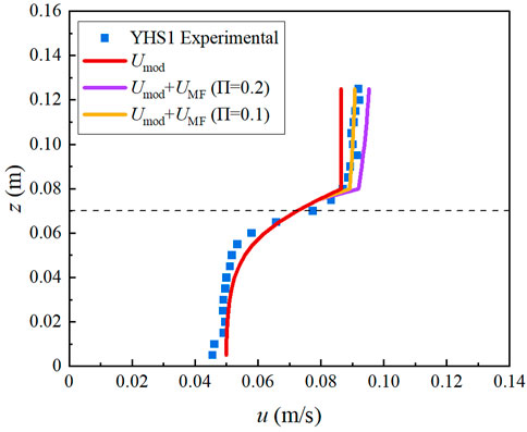
FIGURE 10. The effect of wake term to the velocity model of run YHS1. The black dotted line represents the height of the short vegetation.

7 Conclusion

Through flume experiments using ADV, the flow characteristics of uniform flow with double-layered rigid vegetation are studied, including the longitudinal velocity and lateral vorticity profiles. The proposed model combined the mixing layer concepts in Nikora et al. (2013) and the force balance equations have an acceptable agreement with the experimental data.

(1) In the double-layered vegetation flow, the longitudinal velocity roughly follows a “constant-increasing-constant” distribution vertically. The upper inflection point of the mixing layer zone is found above the height of the short vegetation canopy. When the water depth and vegetation density are the same, the longitudinal velocity has positive tendency with the increasing slope.

(2) It is verified that the velocity profile in zone 2A can be obtained by solving the momentum equation of the balance between the vegetation drag and potential gradient. The velocity in zone 1A and zone B can be predicted by the superposition of the concepts of a uniform velocity distribution in zone 1A (U_UD1) and a hyperbolic tangent profile (U_ML) as the profile in single-layered submerged flexible vegetation flow.

(3) The effects of wake vortices and boundary friction on the velocity model are further explored.

It is worth noting that taking the influence of the vegetation on the gravity-driving term into consideration when solving the force balance equation can describe the velocity profile more precisely. And the velocity model of multi-layered vegetation flow should be further studied based on the research about double-layered vegetation flow in the future.

Data availability statement

The original contributions presented in the study are included in the article/Supplementary Material, further inquiries can be directed to the corresponding authors.

Author contributions

QW, YZ, and PW designed the research. QW, YZ, and TF conducted the experiment. QW wrote the paper. YZ, PW, TF and YB reviewed the paper. All authors read and approved the submitted version.

Funding

The National Natural Science Foundation of China (52179056).

Conflict of interest

The authors declare that the research was conducted in the absence of any commercial or financial relationships that could be construed as a potential conflict of interest.

Publisher’s note

All claims expressed in this article are solely those of the authors and do not necessarily represent those of their affiliated organizations, or those of the publisher, the editors and the reviewers. Any product that may be evaluated in this article, or claim that may be made by its manufacturer, is not guaranteed or endorsed by the publisher.

References

Anjum, N., and Tanaka, N. (2020). Investigating the turbulent flow behaviour through partially distributed discontinuous rigid vegetation in an open channel. River Res. Appl. 36 (8), 1701–1716. doi:10.1002/rra.3671

CrossRef Full Text | Google Scholar

Chen, Z. B., Jiang, C. B., and Nepf, H. M. (2013). Flow adjustment at the leading edge of a submerged aquatic canopy. Water Resour. Res. 49, 5537–5551. doi:10.1002/wrcr.20403

CrossRef Full Text | Google Scholar

Cheng, N. S. (2013). Calculation of drag coefficient for arrays of emergent circular cylinders with pseudofluid model. J. Hydraulic Eng. 139 (6), 602–611. doi:10.1061/(asce)hy.1943-7900.0000722

CrossRef Full Text | Google Scholar

Fan, X. J., Lei, P., Wang, C., and Liu, G. Y. (2020). Influence of flexible submerged vegetation on flow characteristics under different arrangement patterns. J. Huazhong Univ. Sci. Technol. Nat. Sci. Ed. 48 (3), 127–132.

Google Scholar

Huai, W. X., Li, S., Katul, G. G., Liu, M. Y., and Yang, Z. H. (2021). Flow dynamics and sediment transport in vegetated rivers: A review. J. Hydrodynamics 33 (3), 400–420. doi:10.1007/s42241-021-0043-7

CrossRef Full Text | Google Scholar

Huai, W. X., Wang, W. J., Hu, Y., Zeng, Y. H., and Yang, Z. H. (2014). Analytical model of the mean velocity distribution in an open channel with double-layered rigid vegetation. Adv. Water Resour. 69, 106–113. doi:10.1016/j.advwatres.2014.04.001

CrossRef Full Text | Google Scholar

Huai, W. X., Yang, L., Wang, W. J., Guo, Y., Wang, T., and Cheng, Y. (2019). Predicting the vertical low suspended sediment concentration in vegetated flow using a random displacement model. J. Hydrology 578, 124101. doi:10.1016/j.jhydrol.2019.124101

CrossRef Full Text | Google Scholar

Järvelä, J. (2005). Effect of submerged flexible vegetation on flow structure and resistance. J. Hydrology 307, 233–241. doi:10.1016/j.jhydrol.2004.10.013

CrossRef Full Text | Google Scholar

Kubrak, E., Kubrak, J., and Rowinski, P. M. (2008). Vertical velocity distributions through and above submerged, flexible vegetation. Hydrological Sci. J. 53 (4), 905–920. doi:10.1623/hysj.53.4.905

CrossRef Full Text | Google Scholar

Li, D., Yang, Z. H., Zhu, Z. T., Guo, M., Gao, W., and Sun, Z. H. (2020). Estimating the distribution of suspended sediment concentration in submerged vegetation flow based on gravitational theory. J. Hydrology 587, 124921. doi:10.1016/j.jhydrol.2020.124921

CrossRef Full Text | Google Scholar

Li, L., Shi, X., and Li, J. T. (2022). Experimental study on vegetation flow characteristics under rigid-flexible and flexible-rigid patterns. China Rural Water Hydropower 64 (10), 67–73. doi:10.12396/znsd.212119

CrossRef Full Text | Google Scholar

Liu, C., and Nepf, H. (2016). Sediment deposition within and around a finite patch of model vegetation over a range of channel velocity. Water Resour. Res. 52, 600–612. doi:10.1002/2015wr018249

CrossRef Full Text | Google Scholar

Liu, D., Diplas, P., Fairbanks, J. D., and Hodges, C. C. (2008). An experimental study of flow through rigid vegetation. J. Geophys. Res. 113, 4015. doi:10.1029/2008jf001042

CrossRef Full Text | Google Scholar

Liu, D., Diplas, P., Hodges, C. C., and Fairbanks, J. D. (2010). Hydrodynamics of flow through double layer rigid vegetation. Geomorphology 116 (4), 286–296. doi:10.1016/j.geomorph.2009.11.024

CrossRef Full Text | Google Scholar

Nepf, H. (2012). Hydrodynamics of vegetated channels. J. Hydraulic Res. 50 (3), 262–279. doi:10.1080/00221686.2012.696559

CrossRef Full Text | Google Scholar

Nezu, I., and Rodi, W. (1986). Open-channel flow measurements with a laser Doppler anemometer. J. Hydraulic Eng. 112 (5), 335–355. doi:10.1061/(asce)0733-9429(1986)112:5(335)

CrossRef Full Text | Google Scholar

Nikora, N., Nikora, V., and O’Donoghue, T. (2013). Velocity profiles in vegetated open-channel flows: Combined effects of multiple mechanisms. J. Hydraulic Eng. 139, 1021–1032. doi:10.1061/(asce)hy.1943-7900.0000779

CrossRef Full Text | Google Scholar

Qu, G. (2014). “Experimental study on water and sediment transport in open channel flow with vegetation,”. Doctoral dissertation (Wuhan, China: Wuhan University).

Google Scholar

Rahimi, H. R., Tang, X., and Singh, P. (2020). Experimental and numerical study on impact of double layer vegetation in open channel flows. J. Hydrologic Eng. 25 (2), 4019064. doi:10.1061/(asce)he.1943-5584.0001865

CrossRef Full Text | Google Scholar

Singh, P., Rahimi, H. R., and Tang, X. (2019). Parameterization of the modeling variables in velocity analytical solutions of open-channel flows with double-layered vegetation. Environ. Fluid Mech. 19, 765–784. doi:10.1007/s10652-018-09656-8

CrossRef Full Text | Google Scholar

Tang, H. W., Yan, J., and Lu, S. Q. (2007). Advances in research on flows with vegetation in river management. Adv. Water Sci. 18 (5), 785–792. doi:10.3321/j.issn:1001-6791.2007.05.024

CrossRef Full Text | Google Scholar

Tang, X. N., Rahimi, H., Guan, Y. T., and Wang, Y. X. (2021). Hydraulic characteristics of open-channel flow with partially-placed double layer rigid vegetation. Environ. Fluid Mech. 21 (2), 317–342. doi:10.1007/s10652-020-09775-1

CrossRef Full Text | Google Scholar

Truong, S. H., Uijttewaal, W. S. J., and Stive, M. J. F. (2019). Exchange processes induced by large horizontal coherent structures in floodplain vegetated channels. Water Resour. Res. 55, 2014–2032. doi:10.1029/2018wr022954

CrossRef Full Text | Google Scholar

Tseng, C. Y., and Tinoco, R. O. (2021). A two-layer turbulence-based model to predict suspended sediment concentration in flows with aquatic vegetation. Geophys. Res. Lett. 48 (3), 91255. doi:10.1029/2020gl091255

CrossRef Full Text | Google Scholar

Velasco, D., Bateman, A., Redondo, J. M., and Demedina, V. (2003). An open channel flow experimental and theoretical study of resistance and turbulent characterization over flexible vegetated linings. Flow Turbul. Combust. 70 (4), 69–88. doi:10.1023/b:appl.0000004932.81261.40

CrossRef Full Text | Google Scholar

Wang, P., and Cirpka, O. A. (2021). Surface transient storage under low-flow conditions in streams with rough bathymetry. Water Resour. Res. 57 (12), 29899. doi:10.1029/2021wr029899

CrossRef Full Text | Google Scholar

Wang, W. J., Cui, X. Y., Dong, F., Peng, W. Q., Han, Z., Huang, A. P., et al. (2020). Predictions of bulk velocity for open channel flow through submerged vegetation. J. Hydrodyn. 32 (4), 795–799. doi:10.1007/s42241-020-0040-2

CrossRef Full Text | Google Scholar

Wang, W. J., Huai, W. X., Li, S. L., Wang, P., Wang, Y. F., and Zhang, J. (2019b). Analytical solutions of velocity profile in flow through submerged vegetation with variable frontal width. J. Hydrology 578, 124088. doi:10.1016/j.jhydrol.2019.124088

CrossRef Full Text | Google Scholar

Wang, W. J., Huai, W. X., Thompson, S., and Katul, G. G. (2015). Steady nonuniform shallow flow within emergent vegetation. Water Resour. Res. 51 (12), 10047–10064. doi:10.1002/2015wr017658

CrossRef Full Text | Google Scholar

Wang, W. J., Peng, W. Q., Huai, W. X., Katul, G. G., Liu, X. B., Qu, D., et al. (2019a). Friction factor for turbulent open channel flow covered by vegetation. Sci. Rep. 9, 5178. doi:10.1038/s41598-019-41477-7

PubMed Abstract | CrossRef Full Text | Google Scholar

Wang, Z., Li, G. B., He, X. Q., Liu, Y., and Wang, Z. K. (2019c). Water flow resistance characteristics of double-layer vegetation in different submerged states. Water Supply 19 (8), 2435–2442. doi:10.2166/ws.2019.125

CrossRef Full Text | Google Scholar

Xu, Y., and Nepf, H. M. (2020). Measured and predicted turbulent kinetic energy inflow through emergent vegetation with real plant morphology. Water Resour. Res. 56, 27892. doi:10.1029/2020wr027892

CrossRef Full Text | Google Scholar

Xu, Y., and Nepf, H. M. (2021). Suspended sediment concentration profile in a Typha Latifolia Canopy. Water Resour. Res. 57, 29902. doi:10.1029/2021wr029902

CrossRef Full Text | Google Scholar

Yang, J. Q., Kerger, F., and Nepf, H. M. (2015). Estimation of the bed shear stress in vegetated and bare channels with smooth beds. Water Resour. Res. 51, 3647–3663. doi:10.1002/2014wr016042

CrossRef Full Text | Google Scholar

Zhang, J., Wang, W., Shi, H. R., Wang, W. J., Li, Z. B., and Xia, Z. H. (2021). Two-zone analysis of velocity profiles in a compound channel with partial artificial vegetation cover. J. Hydrology 596. doi:10.1016/j.jhydrol.2021.126147doi:126147

CrossRef Full Text | Google Scholar

Zhang, Y. G., Wang, P., Cheng, J. H., Wang, W. J., Zeng, L., and Wang, B. (2020). Drag coefficient of emergent flexible vegetation in steady nonuniform flow. Water Resour. Res. 56 (8), 1–16. doi:10.1029/2020wr027613

CrossRef Full Text | Google Scholar

Zhang, Y. H., and Lai, X. J. (2015). Impact of Vallisneria natans on flow structure. Adv. Water Sci. 26 (1), 99–106. doi:10.14042/j.cnki.32.1309.2015.01.013

CrossRef Full Text | Google Scholar

Zhang, Y. H. (2014). Research progress in effect of vegetation on flow and sediment transport. Wetl. Sci. 12 (5), 669–676. doi:10.13248/j.cnki.wetlandsci.2014.05.020

CrossRef Full Text | Google Scholar

Zhao, F., Huai, W. X., Hu, Y., and Wang, W. J. (2015). Characteristic study of open-channel flow through double layer rigid vegetation. J. Huazhong Univ. Sci. Technol. Nat. Sci. Ed. 43 (01), 85–90. doi:10.13245/j.hust.150118

CrossRef Full Text | Google Scholar

Zhao, F. (2017). “Research on hydraulic characteristics of open channel flows with rigid vegetation,”. Doctoral dissertation (WuhanWuhan, China: Wuhan University).

Google Scholar