 Menghui Li1,2
 Chunmei Geng
 Zhensen Zheng
- 1State Key Laboratory of Environmental Criteria and Risk Assessment, Chinese Research Academy of Environmental Sciences, Beijing, China
- 2State Key Laboratory of Organic Geochemistry, Guangzhou Institute of Geochemistry, Chinese Academy of Sciences, Guangzhou, China
- 3Shandong Zibo Eco-Environmental Monitoring Center, Zibo, China
Ozone variation, excluding meteorological effects, is very important to assess the effects of air pollution control policies. In this study, the Kolmogorov-Zurbenko (KZ) filter method and multiple linear stepwise regression are combined to study the impact of meteorological parameters on ozone concentration over the past 5 years (2016–2020) in a petrochemical industrial city in northern China. Monte Carlo simulations were used to evaluate the reliability for the potential quasi quantitative prediction of the baseline component. The average level of the city and the details of five stations in the city were studied. The results show that the short-term, seasonal, and long-term component variances of maximum daily running average 8 h (MDA8) ozone in Zibo city (City) decomposed by the KZ filter account for 32.06%, 61.67% and 1.15% of the total variance, for a specific station, the values were 32.37%–34.90%, 56.64%–62.00%, and .35%–3.14%, respectively. The average long-term component increase rate is 3.19 μg m−3 yr−1 on average for the city, while it is 1.52–5.95 μg m−3 yr−1 for a specific station. The overall meteorological impact was not stable and fluctuated between −2.60 μg m−3 and +3.77 μg m−3. This difference in trends between the city and specific stations implied that the O3 precursor’s mitigation strategy should be more precise to improve its practical effects.
1 Introduction
Over the past few decades, China’s economic development has seen significant advancements, the pace of urbanization and industrialization has also been accelerating. Accordingly, the consumption of fossil fuels, such as coal and petroleum, has increased significantly, leading to severe air pollution. Haze pollution–characterized by a high concentration of inhalable particulate matter (PM10) and fine particulate matter (PM2.5)–and photochemical smog pollution–characterized by a high concentration of ozone (O3)–were severe issues in the past (Huang et al., 2013; Zhang et al., 2015; Wang et al., 2017; Wang et al., 2019). After the implementation of the “Air Pollution Prevention and Control Action Plan” (also referred to as the “Atmospheric Ten Measures”), the concentration of particulate matter in China has been significantly decreasing each year. However, regional photochemical pollution has become increasingly prominent, and the ozone concentration has risen instead of falling in many cities, and threatens human health, which is of significant concern for the scientific community and relevant government departments (Kuerban et al., 2020; Lin et al., 2021). According to the results of monitoring data from 338 cities in China, the 90th percentile of the maximum daily running average 8 h (MDA8) concentration of ozone increased from 134 μg m−3 in 2015 to 148 μg m−3 in 2019. The proportion of days exceeding the second standard values (160 μg m−3) specified in the National Ambient Air Quality Standards (GB3095–2012), with ozone as the primary pollutant increased from 16.9% in 2015 to 41.7% in 2019, and the proportion of cities exceeding the secondary standard increased from 16% to 30.6% (Ministry of Ecology and Environment of China, 2016, 2019). Research has indicated that the concentration of ozone in 22 of China’s 30 provinces increased from 2015 to 2018, and ozone pollution was prominent and concentrated in the Beijing-Tianjin-Hebei (BTH), Yangtze River Delta (YRD), and Pearl River Delta (PRD) regions (Kuerban et al., 2020).
In comparison to other pollutants, ozone is chemically active and susceptible to meteorological (MET) conditions, such as temperature, relative humidity, wind speed, boundary layer (Cheng et al., 2019; Zong et al., 2021; Zong et al., 2022), and atmospheric transmission. The close relationship between the ozone concentration and meteorological conditions may cover up the ozone long-term trend caused by emission change of ozone precursor. Therefore, it is necessary to filter out the meteorological effects to understand the net impact of emission changes (Rao et al., 1997; Yu et al., 2019). Some methods can help separate the influence of meteorological conditions on ozone, such as Fourier transforms and the wavelet transform method (Eskridge et al., 1997). The Kolmogorov-Zurbenko (KZ) filter, combined with the multiple linear regression (MLR) analysis technique proposed by Rao and Zurbenko (1994) can separate the influence of meteorological conditions on ozone concentration. The KZ filter method is a robust statistical model with a simple algorithm that can be used directly in the presence of missing data (Porter et al., 2001), and is widely used to study ozone pollution trends, such as in Tucson (Wise and Comrie, 2005) and Houston in the United States (Botlaguduru et al., 2018); Canoas and Estio in Brazil (Agudelo-Castaneda et al., 2014); Cessa in the Greek Lee Plain (Papanastasiou et al., 2012); Switzerland (Boleti et al., 2018); and major cities in South Korea (Seo et al., 2014), and Australia, and Spain (Anh et al., 1997; Ibarra-Berastegia et al., 2001; Agudelo-Castaneda et al., 2014), and other places (Kang et al., 2013; Luo et al., 2019). Sa et al. (2015) used the KZ filter method to decompose the original time series of atmospheric pollutants O3, PM10, and NO2 at different time scales, and then ascertained the influence of meteorological conditions on the components of each pollutant through MLR. Research has shown that the KZ filter method can be used to decompose the air pollutants concentrated in metropolises in China, such as BTH (Ma et al., 2016; Gao et al., 2021) and YRD (Yu et al., 2019). Ma et al. (2016) used KZ filtering to remove meteorological influences and extracted the long-term ozone trend of background stations, finding that meteorological conditions have limited effects on the rapid increases in the ozone concentration in Beijing. Research in Hebei province (Gao et al., 2021) has shown that meteorological factors (temperature, atmospheric pressure, and boundary layer height) account for 64% of long-term ozone changes. Therefore, the influence of meteorological factors varies widely in different cities in different periods. Most previous research has focused on the influence of meteorological parameters on regional ozone pollution. However, for ozone pollution control, emission reduction measures should be implemented in every district in each city. It is imperative to investigate whether the effects are similar in all districts within a city. Thus, it is important to evaluate the effect of emission reduction without the influence of meteorological conditions in specific districts within a city.
In this study, Zibo City was selected as a representative heavily-industrial city. Zibo is an important petrochemical industrial city in the North China Plain (NCP), with significant volatile organic compounds (VOCs) emissions (Luo et al., 2018). The KZ filter method and multiple linear stepwise regression are used to study the impact of meteorological parameters on the O3 concentration over a 5-year period (1 1 2016–31 12 2020). Pollutant concentrations on different time scales (long-term, seasonal, and short-term) were obtained, and the influence of meteorological conditions was evaluated quantitatively. The details regarding the long-term component and meteorology impact in each division in the city were discussed. This study will help understand the influence of meteorological conditions on O3 concentration within a city.
2 Materials and methods
2.1 Site description
Zibo is located in the central region of Shandong Province (35°55′20″–37°17′14″N, 117°32′15″–118°31′00″E). It is located in the warm temperate zone, experiencing a semi-humid and semi-arid continental climate; the terrain is high in the south and low in the north, and is surrounded by mountains on three sides—in the east, west, and south. The permanent population was 4.704 million at the end of 2020 (http://www.zibo.gov.cn/).
There are seven national ambient air quality monitoring stations in Zibo. Considering the data integrity of both the O3 concentrations and meteorological parameters, data from five national environmental monitoring stations are selected to study the characteristics at different sites. The five stations are located in five districts: Dongfeng Chemical Plant (DFCP) in Zhangdian District, Putianyuan (PTY) in Linzi District, Qixiangzhan (QXZ) in Zichuan Dictrict, Sanjin Group in Zhoucun District, and Shuangshan (SS) in Boshan District, as shown in Figure 1. Detailed information on these stations can be found in Supplementary Table S1.
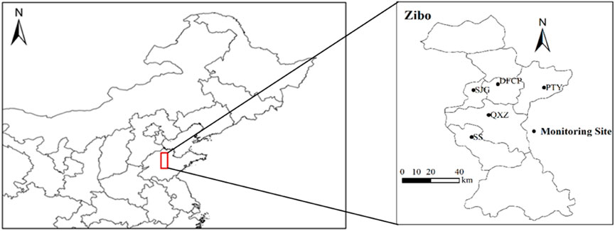
FIGURE 1. Location of the study area and air quality monitoring sites in Zibo City.
2.2 Data acquisition
The daily concentrations of the maximum daily average 8 h (MDA8) ozone for Zibo city (the average conditions of the city) and the five specific sites were obtained from Zibo Environmental Monitoring Center, and the meteorological data was from China National Meteorological Information Centre (http://data.cma.cn/). The data was obtained from 1 January 2016 to 31 December 2020. The meteorological factors used in this study are the daily average relative humidity (RH), daily average wind speed (WS), and daily average temperature (T).
To facilitate a comparison, the ozone concentration of different cities was found and analysed. The ozone concentration data of Beijing (the average value of 12 sites), Tianjin (the average value of 14 sites) and Shijiazhuang (the average value of 7 sites) are from the national real-time air quality release platform of the China National Environmental Monitoring Centre (https://quotsoft.net/air/), and the ozone data of Shanghai (the average value of 19 sites) were collected from Shanghai Municipal Bureau of Ecology and Environment (https://sthj.sh.gov.cn/). Ozone time series data of Los Angeles, California were collected from Air Data at the US Environment Protection Agency (https://www.epa.gov/outdoor-air-quality-data). Available O3 time series data in Berlin (the average value of 3 sites), Paris (the average value of 8 sites) and London (the average value of 6 sites) were obtained from https://discomap.eea.europa.eu/map/fme/AirQualityExport.htm.
2.3 KZ filter method
The KZ filter method was used to decompose the time series of ozone and meteorological conditions. According to Rao and Zurbenko (Rao and Zurbenko, 1994), the original time series of pollutants can be expressed as
Where X(t) represents the original time series, e(t) represents the long-term component, S(t) represents the seasonal component, and W(t) represents the short-term component. In terms of the air quality component, the short-term component can be attributed to the weather and the short-term fluctuations of source emissions, the seasonal component can be attributed to the changes in the angle of the sun, for example, solar radiation, monsoon, temperature and rainfall due to solar angle changes show seasonal variations, and the associated changes in biogenic emissions on a time scale of generally 1a, and the long-term component can be attributed to the changes in source emissions, climate change, policy or economic activities (Rao and Zurbenko, 1994).
The KZ filter method is mainly implemented through the KZA package in R software (Version 4.0.2). It is based on the iterative moving average to eliminate high-frequency changes in the data, which is defined as p applications of a moving average of m points (Rao and Zurbenko, 1994). Its calculation formula is as follows:
Where Yi represents the time series after filtering once, and the calculation is performed again using Yi as the input of the next filter, which iterates p times, and finally yields the filter result KZ(m, p). The unit of the filtered result is the same as that of the original time series; m represents the length of the sliding window (m = 2k+1), k represents the length of the sliding window at both ends when Xi is filtered; X represents the original time series; i represents the sequence (the unit of sampling interval in this study is days); j represents the sliding window variable, which represents the time points involved in the sliding. By adjusting the filter parameters m and p, the filtering of different scale processes can be obtained, and the effective filter width satisfies the following formula:
The above mentioned formula implies that the filter result KZ(m, p) (X) removes high-frequency waves with a wavelength less than N. According to formula (Eq. 3), KZ(15, 5) (X) (the length of the sliding window is 15, and 5 iterations have been carried out) filters out fluctuations with a period less than 33 d (15 × 51/2 ≤ 33); the effective filter width is approximately 33 d (Rao et al., 1997).
Apply meteorological weather and air pollutant quality data to the KZ(15,5) filter, and the extracted time series represent the baseline component, which is defined as the sum of the long-term component and the seasonal component:
The long-term component of the data can be obtained by selecting a KZ filter with a larger window length (Eskridge et al., 1997), and by using the KZ (365, 3) filter (Rao et al., 1997), the long-term component is extracted in the data, and its effective filter width is 632 d, which is about 1.7a. That is, this component filters out fluctuations in the original sequence whose period is less than 632 d (365 × 31/2 ≤ 632).
From the above mentioned functions, the seasonal and short-term components can be calculated as follows:
Ozone is still affected by meteorological conditions after KZ filtering. Linear stepwise regression (Version 22.0, SPSS) is used to eliminate these meteorological effects (Flaum et al., 1996). The decomposed baseline component and short-term component, along with the corresponding decomposed meteorological factors, are introduced into stepwise linear regression, and the O3 statistical model is generated; the corresponding explanatory variance is subsequently given. The robustness of the stepwise linear regression model is tested using 10,000 times Monte Carlo simulation, based on the t distribution of the mean squared error of the model (Xiao et al., 2018). The R2 distribution map is drawn based on this result. It is generally agreed that R2 > .64 indicates that the model has an explanatory degree of 80%. The calculation method for variance explained is as follows (Wise and Comrie, 2005):
Where VE is the explained variance, varX(t) is the variance of the original time series of ozone, and varε(t) is the variance of the residual series. Generally speaking, the smaller the residual sequence, the larger the interpretation variance, and the greater the explanatory power and influence degree of the meteorological conditions participating in the model construction on the time series of ozone.
O3 was measured using online commercial gas analyser (Thermo Scientific 49i, United States), and the measurement method was UV photometric. Previous articles have been published using part of these data, for details see Li et al. (2021). In this study, ground observation data in accordance with the Technical Regulation for Ambient Air Quality Assessment (on trial) (HJ 663-2013) in the data statistical validity provisions, that is, the MDA8 within a natural day is specified as at least 14 valid 8-h average concentration values from 08:00 to 24:00 on that day. When the 14 valid data are not met, if the MDA8 concentration exceeds the concentration standard limit, the statistical results are still valid. For the treatment of missing data, KZ is an iterated moving average and can be used with missing values. Please see the introduction of KZA package in R for details.
3 Results and discussion
3.1 General characteristics of meteorology and ozone concentration
Major MET variables in Zibo City in 2016 and 2020 were compared. The monthly variation in (a) temperature, (b) relative humidity, and (c) wind speed in Zibo City in 2016 and 2020 are illustrated in Supplementary Figure S1. The annual average wind speed and relative humidity decreased (by .25 m/s and .79%, respectively), and the annual average temperature remained basically unchanged (14.3°C in 2016 and 14.2°C in 2020). The changes in the MET conditions will affect the concentration of pollutants. Therefore, it is of great significance to understand the effects of the MET conditions on the concentrations of pollutants to eliminate them.
The 90th percentile of MDA8 of the ozone concentration in Zibo City from 2016 to 2020 is between 184 and 203 μg m−3, exceeding the secondary standard limit (160 μg m−3) by 1.15–1.27 times. The annual ozone concentration reached a maximum in 2019 and a minimum in 2017. Another cumulative index for human health, the annual Sum of Ozone Means Over 35 ppb (SOMO35), was 1.27 × 10⁴ ppb d–1.74 × 10⁴ ppb d (1.55 × 10⁴ ppb d, on average) from 2016 to 2020, which was higher than the highest SOMO35 (6.8 × 10³ ppb d) reported in the southeastern Unites States in 2000 (Ellingsen et al., 2008), as well as the observed value (1.5 × 10³–6.0 × 10³) in France (Sicard et al., 2016).
In terms of monthly variations, as shown in Figure 2, the MDA8 is relatively high from April to September, while the MDA8 is relatively low from December to March of the following year. The highest MDA8 usually appeared in June and July. In terms of daily variations, the concentration of MDA8 ozone varies greatly, ranging from 9 to 274 μg m−3. In terms of the inter-annual variation, an increasing trend can be observed. The overall variations of six percentiles (5%, 25%, 50%, 75%, 95% and 99%) based on the MDA8 ozone statistics were +2.2, +4.0, +4.5, +4.2, and +5.2 μg m−3 for the whole city during 2016–2020, indicating increases in all data segments and a relatively faster increase at the upper end of the ozone distribution.
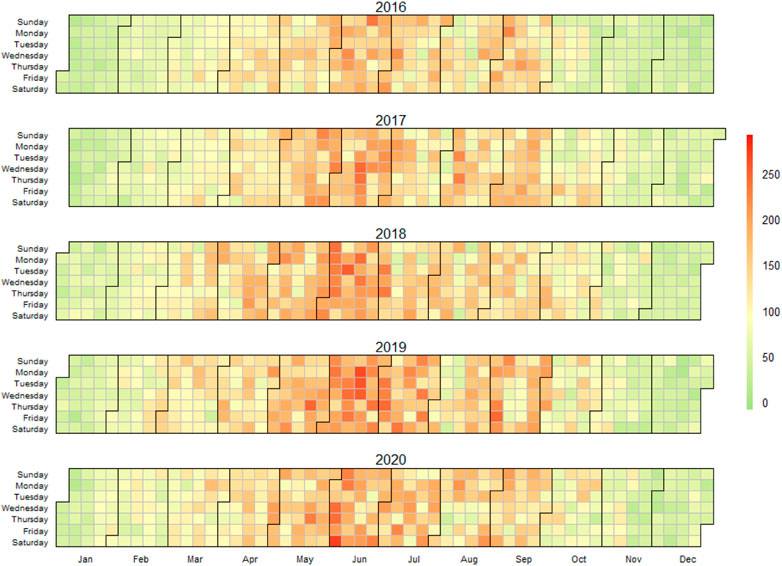
FIGURE 2. Calendar heat map of MDA8 ozone of Zibo city during 2016–2020.
In addition, the time when the MDA8 ozone concentration exceeded the secondary standard limit (160 μg m−3) appeared earlier every year from 2016 to 2019. The first day of MDA8 exceeding 160 μg m−3 occurred on 30 April in 2016, on 7 April in 2017, on 25 March in 2018, on 10 March in 2019 and on 23 March in 2020. The MDA8 ozone concentration fluctuated greatly in the summer and remained relatively stable in winter.
3.2 O3 time series after KZ filtering
3.2.1 Separated time series of MDA8 ozone
KZ filtering was performed on the MDA8 of the ozone sequence of Zibo City (Figure 3) and five sites (Supplementary Figure S2) to obtain the short-term, seasonal and long-term component sequences. It can be seen that, for all cases, there is high-frequency noise in the original time series of MDA8 ozone, which exhibits obvious seasonal characteristics. After removing the short-term component, caused by meso-scale and synoptic-scale meteorological processes (Yu et al., 2019), the seasonal component presents clearer and smoother periodic characteristics, with a trough from December to January of the following year, and with a peak in June. Every site in each year exhibited obvious bimodal peaks. In general, peaks occurred in June and September, and dips occurred in July or August. Owing to the influence of the monsoon climate, the precipitation was mainly concentrated from July to August. For example, the sum of the average precipitation in July to August from 2016 to 2020 was 373.2, 283.9, 422.6, 621.1, and 347.3 mm, respectively, accounting for 52.39%, 56.57%, 45.92%, 78.64% and 48.14% of the total annual average precipitation (Zibo City Statistical Yearbook, 2016, 2017, 2018, 2019, 2020). In additional to the precipitation, the high relative humidity, low temperature, cloudy days, and the clearance of the precursor also weaken the ozone formation (Boleti et al., 2018; Lin et al., 2021).

FIGURE 3. Separated time series of MDA8 of the ozone values during 2016–2020. (A) the original data; (B) the short-term component; (C) the seasonal component; (D) the long-term component.
The long-term component clearly exhibits an upward trend of MDA8 ozone, and this trend is covered in the original time series by high-frequency noise (Yu et al., 2019). The variation shows an obvious increase in the study period for all cases, followed by a smooth or small fluctuation trend. The growth rates of the long-term component of the city is 3.19 μg m−3 yr−1 from 2016 to 2020. The growth rates of the long-term components of the DFCP, QXZ, PTY, SJG, and SS stations are 1.52, 1.61, 1.97, 1.99, and 5.95 μg m−3 yr−1, respectively. The increase rate of the city is higher than the 2.42 μg m−3 yr−1 rate of the SDZ background station in Beijing (Ma et al., 2016), and is lower than the average value of 3.85 μg m−3 yr−1 in the YRD region during 2013–2017 (Yu et al., 2019).
The long-term component of MDA8 ozone for the city from 2016 to 2020 was compared with the long-term component of MDA8 ozone in Los Angeles from 1990 to 2020, and Beijing, Tianjin, Shijiazhuang, Shanghai, London, Paris, and Berlin in recent years (Figure 4). The trend of the long-term component of MDA8 ozone for compared cities was similar to those found in previous studies (Yu et al., 2020), which proves that our MLR method is reliable. In comparison to London, Paris, and Berlin, the concentration level in the selected cities in China was much higher. Further, there was a large increase from 2017 to 2019 for the long-term component trend of MDA8 ozone in this study, which is similar to that in Shijiazhuang, Tianjin, and Los Angeles in the early 21st century but in different years.
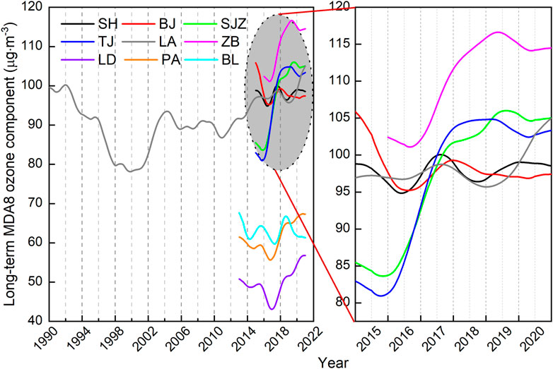
FIGURE 4. Evolution of urban surface MDA8 ozone levels in different cities. SH, Shanghai, BJ, Beijing, SJZ, Shijiazhuang, TJ, Tianjin, LA, Los Angeles, ZB, Zibo, LD, London, PA, Paris, BL, Berlin.
3.2.2 Contribution of each component to the total variance
To identify the contribution of each temporal component to the original ozone data, the variance of each generated time series was calculated and the contribution to the total variance of the original data was determined as shown in Table 1. Ideally, the long-term component, the seasonal component, and the short-term component should be independent of each other, that is, the variance of the original time series should be equal to the sum of the three component variances (Ibarra-Berastegia et al., 2001). The higher the sum of the contribution rate of each component to the variance of the total variance, the better the decomposition effect after filtering. The results from Table 1 show that the sum of the variance of the short-term, seasonal, and long-term components of MDA8 of ozone after KZ filter decomposition contributes 94.56%–95.06% to the variance of the original time series, indicating that the components basically meet the conditions of mutual independence.
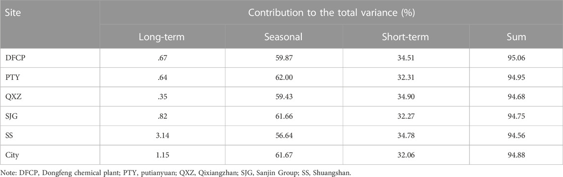
TABLE 1. Contribution of the KZ filter to the total variance of each component in the original MDA8 ozone.
The seasonal component contributes the most to the total variance of the original MDA8 ozone sequence (61.67%), followed by the short-term component (32.06%) and the long-term component (1.15%), demonstrating that ground ozone concentrations in the city were mainly affected by the variations in the seasonal and short-term meteorological conditions. These contributions were consistent with these found in previous studies (Ma et al., 2016; Cheng et al., 2019; Yu et al., 2019). For example, Ma (Ma et al., 2016) used KZ filtering to analyse the MDA8 of ozone of Beijing Shangdianzi (SDZ) background station from 2003 to 2015, revealing that the total variance of the seasonal and short-term component accounted for 57.6% and 36.4%, respectively.
It can be seen from Table 1 that the contribution of seasonal and short-term component dominated the variation of ozone for each station, with certain differences. For the SS site, the long-term component (3.14%) is significantly higher than that of the other four sites (.62% on average), while the seasonal component of the SS site (56.64%) is lower than that of the other four sites (average 60.71%). The long-term component represents the combined effects of different factors, such as pollutant emissions, climate change, and socioeconomic development. This site (SS) is located on a hill at an elevation of about 150 m, within 1 km radium, there is a main road on the west sides, and no other obvious sources of contamination. Relative to the other urban sites, the SS site is at higher altitude and may be more influenced by climate and atmospheric circulation in the long term. Therefore, the long-term component contribution of this site is large compared to other sites.
3.3 Quantitative assessment of the long-term impact of meteorological conditions
3.3.1 Multiple linear stepwise regression and robustness test
The time series decomposed by KZ filtering is still affected by some meteorological conditions, and multiple linear stepwise regression is an effective measure to further eliminate meteorological conditions (Flaum et al., 1996). The filtered ozone time series was set as the dependent variable, and the filtered meteorological variable time series was set as the independent variable. By using multiple linear stepwise regression (SPSS 22.0), the model between the ozone and the meteorological conditions was established in terms of the baseline component and the short-term component, and the relationship formula is as follows (Cheng et al., 2019)
Where W(t) and wi(t) are the short-term components of ozone and the ith meteorological conditions respectively. a0 and ai are regression coefficients. εw(t) is the regression residual of the short-term component. Xb(t) and xi(t) are the baseline components of ozone and the ith meteorological conditions, respectively. b0 and bi are regression coefficients. εb(t) is the regression residual of the baseline component.
Table 2 shows the statistical model of multiple linear stepwise regression and the corresponding explanatory variance (Gao, et al., 2021). In terms of baseline components, the three meteorological factors explained 89.98% of the total ozone variance in the city, and the value ranged from 86.82% to 90.62% for the five sites. Temperature was positively correlated with MDA8 ozone and relative humidity was negatively correlated with MDA8 ozone. The coefficient of temperature was much higher than that of relative humidity. For wind speed, negative correlations existed for the city, which is consistent with the general finding that a high wind speed facilitates diffusion. However, for specific sites, positive correlations exist between wind speed and MDA8 ozone, which points to significant differences between sites. Monte Carlo simulation (Figure 5A, Supplementary Figure S3) shows that the simulated R2 surpassed .64 for over 95% of the baseline component, indicating that the model might be reliable for potential quasi-quantitative prediction of the baseline component.
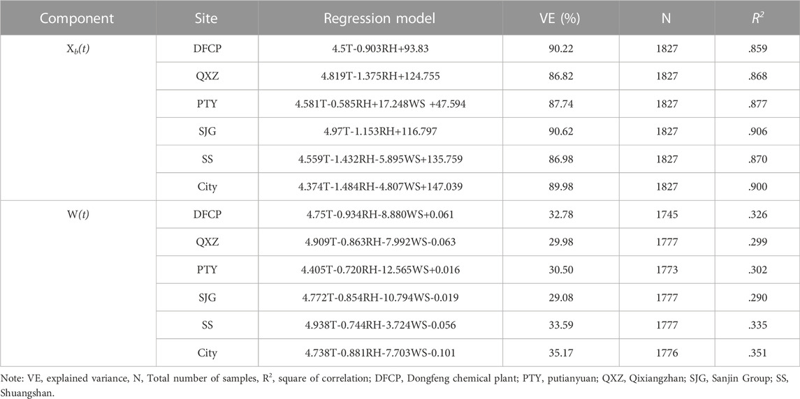
TABLE 2. Stepwise regression model for the baseline and short-term components of MDA8 ozone.
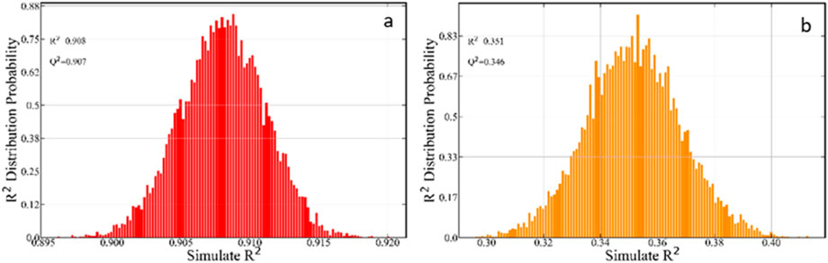
FIGURE 5. The results of 10,000 times Monte Carlo simulation based on the t distribution of the mean squared errors of the baseline component (A) and short-term component (B) regression models in the city.
For the short-term component, the relationship between the ozone and the meteorological variables is relatively low, and the explained variance was 29.08%–33.59% (35.17% on average) for all monitoring sites. For this component, wind speed presents the highest explained variance, indicating that wind speed has a great impact on ozone over the short term. Monte Carlo simulation (Figure 5B) shows that the simulated R2 is widely distributed between 0 and 1, and is smaller than .5 for all cases, indicating that the regression model was less robust (Xiao, et al., 2018).
3.3.2 Reconstruction of long-term ozone component time series
According to Eqs 9, 10, the fitting value of the short-term and the baseline component of ozone can be obtained, and it can be considered that the sum of the short-term and the baseline component primarily reflects the influence of meteorological factors. The residual error between the observed value of ozone and the fitted value is expressed as follows:
The residual sequence ε(t) mainly represents ozone fluctuations caused by the changes in the emissions from the pollution source, but the series still contains the influence of meteorological conditions that are not considered in the regression fitting; further, there are also contributions from modelling errors and monitoring errors of ozone. In view of these factors, KZ (m=365, p=3) is used to filter ε(t) again, and the filter result εLT(t) represents the long-term change trend of ozone caused only by changes in the pollution source emissions. Although εLT(t) is filtered, it is still a residual sequence. To intuitively reflect the long-term component changes of O3 caused by pollution emissions, XLT(t) is reconstructed (Cheng et al., 2019)
Where
Figure 6 shows the variation of the long-term ozone component before and after meteorological adjustment. The red curve represents the long-term change trend of the ozone component after the meteorological influence is eliminated. This series only reflects the variation caused by pollutant emissions. It can be seen that, due to the variation in pollutant emissions, the long-term component of ozone for the city exhibited an overall upward trend in 2016–2018 and a downward trend in 2019–2020. In 2018, the People’s Government of Zibo issued the “Three-Year Implementation Plan for Zibo to Win the Blue Sky Defense War (2018–2020),” which pointed out that the trend of rising O3 concentration must be significantly curbed by 2020 (http://www.zibo.gov.cn). This indicates that the action plan that began in 2018 has greatly reduced anthropogenic emissions in the city. In terms of the specific districts, the long-term component of ozone in the PTY site exhibited an upward in 2016–2018 and a downward trend in 2019–2020. The QXZ site exhibited a downward trend in 2016, an upward trend in 2017–2018, and no significant variation in 2019–2020. In addition, the SS site does not change much after the meteorological impact is eliminated. This is because the site is a hillside site with a high altitude, relatively good diffusion conditions, relatively large surrounding vegetation coverage, and has less impact from anthropogenic emissions.
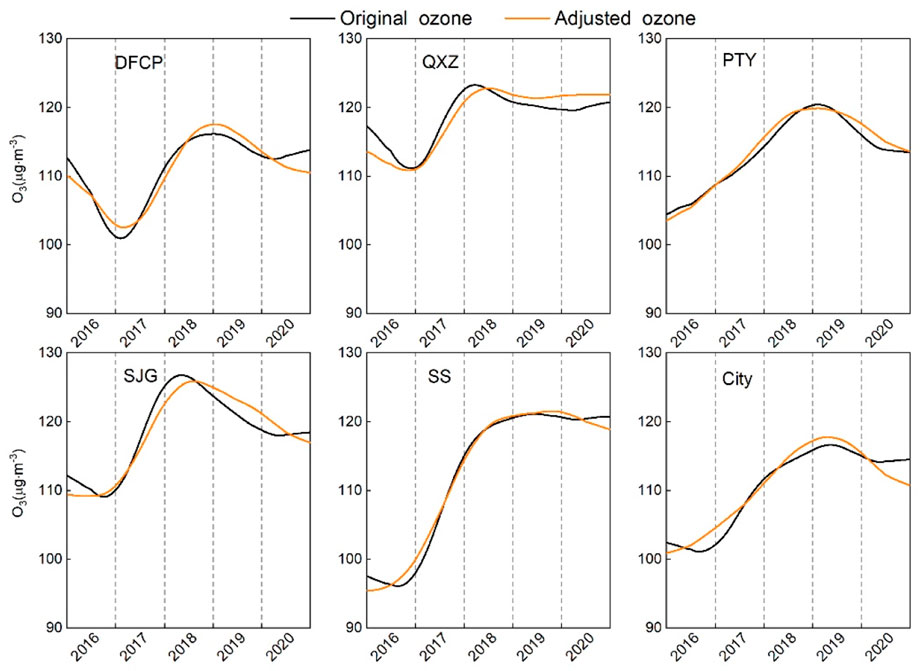
FIGURE 6. Variation in the ozone long-term component before and after meteorological adjustment. DFCP, Dongfeng Chemical Plant site, QXZ, Qixiangzhan, PTY, Putianyuan site, SJG, Sanjin Group site, SS, Shuangshan site and City: Zibo city.
The impact of meteorological conditions on the long-term component of ozone can be expressed more directly by calculating the difference between the long-term components before and after adjustment, as shown in Figure 7. If the difference (the ozone concentration before adjustment minus that after) is positive, the meteorological condition does not favour ozone generation. For the city, during the periods from January to May 2016, from July 2017 to April 2018, and from March 2020 to December 2020, the meteorological conditions are not conductive to the improvement of ozone concentrations, increasing the long-term component of ozone by .69, .38, and 2.11 μg m−3, respectively. However, from June 2016 to July 2017 and from May 2018 to February 2020, the meteorological conditions are conducive to the abatement of ozone, reducing the long-term components of ozone by 1.62 and .95 μg m−3, respectively. The overall meteorological impact was not stable and fluctuated between −2.60 and +3.77 μg m−3.
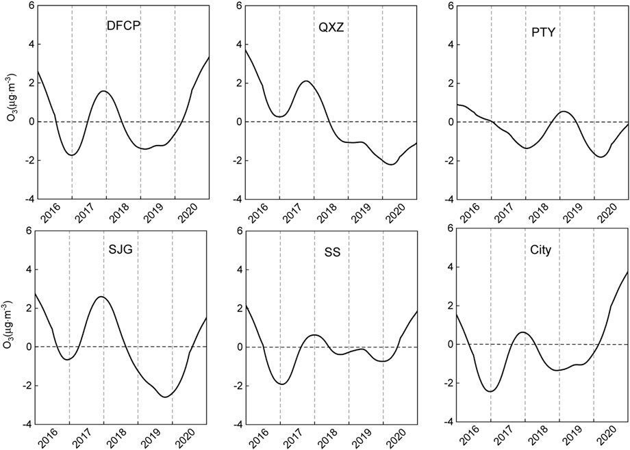
FIGURE 7. Assessment of the influence of weather conditions on the long-term variation of ozone in the city and five districts within the city. DFCP, Dongfeng Chemical Plant site, QXZ, Qixiangzhan, PTY, Putianyuan site, SJG, Sanjin Group site, SS, Shuangshan site and City: Zibo city.
4 Conclusion
KZ filtering is used to decompose the ozone time series into long-term, seasonal, and short-term components in Zibo City and the five stations in this city. Monte Carlo simulation was used to evaluate the reliability of the potential quasi-quantitative prediction of the baseline component. The impact of meteorological parameters on the ozone concentration for the past 5 years (2016–2020) was studied.
The seasonal component contributes the most to the total variance of the original MDA8 ozone sequence (61.67%), followed by the short-term component (32.06%) and the long-term component (1.15%). The growth rate of the long-term component in the city is 3.19 μg m−3 yr−1 from 2016 to 2020. The growth rates of the long-term component for the DFCP, QXZ, PTY, SJG, and SS stations are 1.52, 1.61, 1.97, 1.99, and 5.95 μg m−3 yr−1, respectively. After the meteorological adjustment, the long-term component of ozone for the city exhibited an overall upward trend in 2016–2018 and a downward trend in 2019–2020. This transition time was consistent with the implementation of the Blue Sky Defense Action Plan, which began in 2018. The overall meteorological impact was not stable and fluctuated between −2.60 and +3.77 μg m−3.
In this study, the time period was from 2016 to 2020, as the O3 monitoring started in 2016 for all cities in China. When more data is available, further evaluations should be conducted. In addition, if more data is available, the influence of solar radiation, the dew-point, the boundary layer height and other pollutants on O3 concentration could also be analysed using the method in this study.
Data availability statement
The original contributions presented in the study are included in the article/Supplementary Material, further inquiries can be directed to the corresponding authors.
Author contributions
ML, CG, and XW designed the research and led the overall scientific questions. LL, WY, and BX carried out data processing and analysis. ZZ helped with code programming. ML wrote the manuscript and then CG and XW revised the manuscript. All authors read and approved the submitted version.
Funding
This work was supported by Center for Air Pollution Prevention and Control (Nos. DQGG202119 and DQGG202137).
Conflict of interest
The authors declare that the research was conducted in the absence of any commercial or financial relationships that could be construed as a potential conflict of interest.
Publisher’s note
All claims expressed in this article are solely those of the authors and do not necessarily represent those of their affiliated organizations, or those of the publisher, the editors and the reviewers. Any product that may be evaluated in this article, or claim that may be made by its manufacturer, is not guaranteed or endorsed by the publisher.
Supplementary material
The Supplementary Material for this article can be found online at: https://www.frontiersin.org/articles/10.3389/fenvs.2022.1081453/full#supplementary-material
References
Agudelo-Castaneda, D. M., Teixeira, E. C., and Pereira, F. N. (2014). Time–series analysis of surface ozone and nitrogen oxides concentrations in an urban area at Brazil. Atmos. Pollut. Res. 5, 411–420. doi:10.5094/APR.2014.048
Anh, V., Duc, H., and Azzi, M. (1997). Modeling anthropogenic trends in air quality data. J. Air Waste Manage. Assoc. 47 (1), 66–71. doi:10.1080/10473289.1997.10464406
Boleti, E., Hueglin, C., and Takahama, S. (2018). Ozone time scale decomposition and trend assessment from surface observations in Switzerland. Atmos. Environ. 191, 440–451. doi:10.1016/j.atmosenv.2018.07.039
Botlaguduru, V. S. V., Kommalapati, R. R., and Huque, Z. (2018). Long-term meteorologically independent trend analysis of ozone air quality at an urban site in the greater Houston area. J. Air Waste Manage. Assoc. 68, 1051–1064. doi:10.1080/10962247.2018.1466740
Cheng, N. L., Li, R. Y., Xu, C. X., Chen, Z. Y., Chen, D. L., Meng, F., et al. (2019). Ground ozone variations at an urban and a rural station in Beijing from 2006 to 2017: Trend, meteorological influences and formation regimes. J. Clean. Prod. 235, 11–20. doi:10.1016/j.jclepro.2019.06.204
Ellingsen, K., Gauss, M., Dingenen, R. V., Dentener, F. J., Emberson, L., Fiore, A. M., et al. (2008). Global ozone and air quality: A multi-model assessment of risks to human health and crops. Atmos. Chem. Phys. Discuss. 8, 2163–2223. doi:10.7916/D8M32VD4
Eskridge, R. E., Ku, J. Y., Rao, S. T., Porter, P. S., and Zurbenko, I. G. (1997). Separating different scales of motion in time series of meteorological variables. Bull. Am. Meteorol. Soc. 78, 1473–1483. doi:10.1175/1520-0477(1997)078<1473:sdsomi>2.0.co;2
Flaum, J. B., Rao, S. T., and Zurbenko, I. G. (1996). Moderating the influence of meteorological conditions on ambient ozone concentrations. J. Air Waste Manage. Assoc. 46, 35–46. doi:10.1080/10473289.1996.10467439
Gao, S., Bai, Z. P., Liang, S., Yu, H., Chen, L., Sun, Y. L., et al. (2021). Simulation of surface ozone over Hebei province, China using Kolmogorov-Zurbenko and artificial neural network (KZ-ANN) combined model. Atmos. Environ. 261, 118599. doi:10.1016/j.atmosenv.2021.118599
Huang, J. P., Zhou, C. H., Lee, X. H., Bao, Y. X., Zhao, X. Y., Fung, J., et al. (2013). The effects of rapid urbanization on the levels in tropospheric nitrogen dioxide and ozone over East China. Atmos. Environ. 77, 558–567. doi:10.1016/j.atmosenv.2013.05.030
Ibarra-Berastegia, G., Madariagab, I., Elıasb, A., Agirrec, E., and Uria, J. (2001). Long-term changes of ozone and traffic in Bilbao. Atmos. Environ. 35, 5581–5592. doi:10.1016/S1352-2310(01)00210-2
Kang, D. W., Hogrefe, C., Foley, K. L., Napelenok, S. L., Mathur, R., and Rao, S. T. (2013). Application of the Kolmogorov–Zurbenko filter and the decoupled direct 3D method for the dynamic evaluation of a regional air quality model. Atmos. Environ. 80, 58–69. doi:10.1016/j.atmosenv.2013.04.046
Kuerban, M., Waili, Y., Fan, F., Liu, Y., Qin, W., Dore, A. J., et al. (2020). Spatio-temporal patterns of air pollution in China from 2015 to 2018 and implications for health risks. Environ. Pollut. 258, 113659. doi:10.1016/j.envpol.2019.113659
Li, K. W., Wang, X. H., Li, L. M., Wang, J., Liu, Y. Y., Cheng, X., et al. (2021). Large variability of O3-precursor relationship during severe ozone polluted period in an industry-driven cluster city (Zibo) of North China Plain. J. Clean. Prod. 316, 128252. doi:10.1016/j.jclepro.2021.128252
Lin, C. Q., Lau, A. K. H., Fung, J. C. H., Song, Y. S., Li, Y., Tao, M. H., et al. (2021). Removing the effects of meteorological factors on changes in nitrogen dioxide and ozone concentrations in China from 2013 to 2020. Sci. Total Environ. 793, 148575. doi:10.1016/j.scitotenv.2021.148575
Luo, H., Astithaa, M., Hogrefe, C., Mathurb, R., and Rao, S. T. (2019). A new method for assessing the efficacy of emission control strategies. Atmos. Environ. 199, 233–243. doi:10.1016/j.atmosenv.2018.11.010
Luo, Y. Y., Zhou, X. H., Zhang, J. Z., Xiao, Y., Wang, Z., Zhou, Y., et al. (2018). PM2.5 pollution in a petrochemical industry city of northern China: Seasonal variation and source apportionment. Atmos. Res. 212, 285–295. doi:10.1016/j.atmosres.2018.05.029
Ma, Z. Q., Xu, J., Quan, W. J., Zhang, Z. Y., Lin, W. L., and Xu, X. B. (2016). Significant increase of surface ozone at a rural site, north of eastern China. Atmos. Chem. Phys. 16, 3969–3977. doi:10.5194/acp-16-3969-2016
Papanastasiou, D. K., Melas, D., Bartzanas, T., and Kittas, C. (2012). Estimation of ozone trend in central Greece, based on meteorologically adjusted time series. Environ. Model Assess. 17, 353–361. doi:10.1007/s10666-011-9299-6
Porter, P. S., Rao, S. T., Zurbenko, I. G., Dunker, A. M., and Wolff, G. T. (2001). Ozone air quality over north America: Part II—an analysis of trend detection and attribution techniques. J. Air Waste Manage. Assoc. 51 (2), 283–306. doi:10.1080/10473289.2001.10464261
Rao, S. T., and Zurbenko, I. G. (1994). Detecting and tracking changes in ozone air quality. J. Air Waste Manage. Assoc. 44, 1089–1092. doi:10.1080/10473289.1994.10467303
Rao, S. T., Zurbenko, I. G., Neagu, R., Porter, P. S., Ku, J. Y., and Henry, R. F. (1997). Space and time scales in ambient ozone data. Bull. Am. Meteorol. Soc. 78, 2153–2166. doi:10.1175/1520-0477(1997)078<2153:satsia>2.0.co;2
Sa, E., Tchepel, O., Carvalho, A., and Borrego, C. (2015). Meteorological driven changes on air quality over Portugal: A KZ filter application. Atmos. Pollut. Res. 6, 979–989. doi:10.1016/j.apr.2015.05.003
Seo, J., Youn, D., Kim, J. Y., and Lee, H. (2014). Extensive spatiotemporal analyses of surface ozone and related meteorological variables in South Korea for the period 1999–2010. Atmos. Chem. Phys. 14, 6395–6415. doi:10.5194/acp-14-6395-2014
Sicard, P., Serra, R., and Rossello, P. (2016). Spatiotemporal trends in ground-level ozone concentrations and metrics in France over the time period 1999–2012. Environ. Res. 149, 122–144. doi:10.1016/j.envres.2016.05.014
Wang, N., Lyu, X. P., Deng, X. J., Huang, X., Jiang, F., and Ding, A. J. (2019). Aggravating O3 pollution due to NOx emission control in eastern China. Sci. Total Environ. 677, 732–744. doi:10.1016/j.scitotenv.2019.04.388
Wang, T., Xue, L. K., Brimblecombe, P., Lam, Y. F., Li, L., and Zhang, L. (2017). Ozone pollution in China: A review of concentrations, meteorological influences, chemical precursors, and effects. Sci. Total Environ. 575, 1582–1596. doi:10.1016/j.scitotenv.2016.10.081
Wise, E. K., and Comrie, A. C. (2005). Meteorologically adjusted urban air quality trends in the Southwestern United States. Atmos. Environ. 39, 2969–2980. doi:10.1016/j.atmosenv.2005.01.024
Xiao, K., Shen, Y. X., Liang, S., Tan, J. H., Wang, X. M., Liang, P., et al. (2018). Characteristic regions of the fluorescence excitation–emission matrix (EEM) to identify hydrophobic/hydrophilic contents of organic matter in membrane bioreactors. Environ. Sci. Technol. 52, 11251–11258. doi:10.1021/acs.est.8b02684
Yu, Y. J., Meng, X. Y., Wang, Z., Zhou, W., and Yu, H. X. (2020). Driving factors of the significant increase in surface ozone in the Beijing-Tianjin-Hebei region, China, during 2013-2018. Environ. Sci. 41 (1), 106–114. doi:10.13227/j.hjkx.201905222
Yu, Y. J., Wang, Z., He, T., Meng, X. Y., Xie, S. Y., and Yu, H. X. (2019). Driving factors of the significant increase in surface ozone in the Yangtze River Delta, China, during 2013–2017. Atmos. Pollut. Res. 10, 1357–1364. doi:10.1016/j.apr.2019.03.010
Zhang, Z. Y., Zhang, X. l., Gong, D. Y., Quan, W. J., Zhao, X. J., Ma, Z. Q., et al. (2015). Evolution of surface O3 and PM2.5 concentrations and their relationships with meteorological conditions over the last decade in Beijing. Atmos. Environ. 108, 67–75. doi:10.1016/j.atmosenv.2015.02.071
Zong, L., Yang, Y. J., Gao, M., Wang, H., Wang, P., Zhang, H. L., et al. (2021). Large-scale synoptic drivers of co-occurring summertime ozone and PM2.5 pollution in eastern China. Atmos. Chem. Phys. 21, 9105–9124. doi:10.5194/acp-21-9105-2021
Keywords: ozone, KZ filter, meteorological conditions, multiple linear regression, Monte Carlo simulation
Citation: Li M, Geng C, Li L, Zheng Z, Xu B, Yang W and Wang X (2023) Meteorological impacts on surface ozone: A case study based on Kolmogorov–Zurbenko filtering and multiple linear regression. Front. Environ. Sci. 10:1081453. doi: 10.3389/fenvs.2022.1081453
Received: 27 October 2022; Accepted: 14 December 2022;
Published: 06 January 2023.
Edited by:
Gen Zhang, Chinese Academy of Meteorological Sciences, ChinaReviewed by:
Yuanjian Yang, Nanjing University of Information Science and Technology, ChinaHaipeng Lin, Harvard University, United States
Copyright © 2023 Li, Geng, Li, Zheng, Xu, Yang and Wang. This is an open-access article distributed under the terms of the Creative Commons Attribution License (CC BY). The use, distribution or reproduction in other forums is permitted, provided the original author(s) and the copyright owner(s) are credited and that the original publication in this journal is cited, in accordance with accepted academic practice. No use, distribution or reproduction is permitted which does not comply with these terms.
*Correspondence: Chunmei Geng, Z2VuZ2NtQGNyYWVzLm9yZy5jbg==; Xinhua Wang, d2FuZ3hoQGNyYWVzLm9yZy5jbg==